Statistical Mechanics of Online Learning of Drifting Concepts : A Variational Approach.

Abstract

We review the application of Statistical Mechanics methods to the study of online learning of a drifting concept in the limit of large systems. The model where a feed-forward network learns from examples generated by a time dependent teacher of the same architecture is analyzed. The best possible generalization ability is determined exactly, through the use of a variational method. The constructive variational method also suggests a learning algorithm. It depends, however, on some unavailable quantities, such as the present performance of the student. The construction of estimators for these quantities permits the implementation of a very effective, highly adaptive algorithm. Several other algorithms are also studied for comparison with the optimal bound and the adaptive algorithm, for different types of time evolution of the rule.

I Introduction

The importance of universal bounds to generalization errors, in the spirit of the Vapnik-Chervonenkis (VC) theory, cannot be overstated, since these results are independent of target function and input distribution. This bounds are tight in the sense that for a particular target an input distribution can be found where generalization is as difficult as the VC bound states. However for several learning problems, by making specific assumptions, it is possible to go further. Haussler et al [11] have found tighter bounds that even capture functional properties of learning curves, such as for example the occurrence of discontinuous jumps in learning curves, which cannot be predicted from VC theory alone.

These results were derived by adapting to the problem of learning, ideas that arise in the context of Statistical Mechanics. In recent years many other results [26, 32, 23], bounds or approximations, rigorous or not, have been obtained in the learning theory of neural networks by applying a host of methods originated in the study of disordered materials. These methods permit looking at the properties of large networks, where great analytical simplifications can occur; and also, they afford the possibility of performing averages over the randomness introduced by the training data. They are useful in that they give information about typical rather than e.g. worst case behavior and should be regarded as complementary to those of Computational Learning Theory.

The Statistical Mechanics of learning has been formulated either as a problem at thermodynamical equilibrium or as a dynamical process off-equilibrium, depending on the type of learning strategy. Although many intermediate regimes can be identified, we briefly discuss the two dynamical extremes. Batch or offline methods essentially give rise to the equilibrium formulation, while online learning can be better described as an off equilibrium process.

The offline method begins by constructing a cost or energy function on the parameter space, which depends on all the training data simultaneously [26, 32]. Learning occurs by defining a gradient descent process on the parameter space, subject to some (thermal) noise process, which permits to some extent escaping from local traps. In a very simplified way it may be said that, after some time, this process leads to “Thermal equilibrium”, when essentially all possible information has been extracted by the algorithm from the learning set. The system is now described by a stationary (Gibbs) probability distribution on parameter space.

On the other extreme lies online or incremental learning. Instead of training with a cost function defined over all the available examples, the online cost function depends directly on only one single example, independently chosen at each time step of the learning dynamics [1],(for a review, [22]). Online learning occurs also by gradient descent, but now the random nature of the presentation of the examples implies that at each learning step an effectively different cost function is being used. This can lead to good performances even without the costly memory resources needed to keep the information about the whole learning set, as is the case in the offline case.

Although most of the work has concentrated on learning in stationary environments with either online or offline strategies, the learning of drifting concepts has also been modeled using ideas of Statistical Mechanics [3, 4, 17]. The natural approach to this type of problem is to consider online learning, since old examples may not be representative of the present state of the concept. It makes little sense, if any, to come to thermal equilibrium with possibly already irrelevant old data, as would be the case of an offline strategy. The possibility of forgetting old information and of preventing the system from reusing it, which are essential features to obtain good performance, are inherent to the online processes we will see below.

We will model the problem of supervised learning, in the sense of Valiant [29], of a drifting concept by defining a “teacher” neural network. Drift is modeled by allowing the teacher network parameters to undergo a drift that can be either random or deterministic. The dynamics of learning occurs in discrete time. At each time step, a random input vector is chosen independently from a distribution $P_{D}$, giving rise to a temporal stream of input-output pairs, where the output is determined by the teacher. From this set of data the student parameters will be built.

The question addressed in this paper concerns the best possible way in which the information can be used by the student in order to obtain maximum typical generalization ability. This is certainly too much to ask for and we will have to make some restrictions to the problem. This question will be answered by means of a variational method for the following class of exactly soluble models: a feed-forward boolean network learning from a teacher which is itself a neural network of similar architecture and learns by a hebbian modulated mechanism.

This is still hard and further restrictions will be made. The thermodynamic limit (TL) will always be assumed. This means that the dimension $N$ of parameter space is taken to infinity. This increase brings about great analytical simplifications. The TL is the natural regime to study in Condensed Matter Physics. There the number of interacting units is of the order of $N\approx 10^{23}$ and fluctuations of macroscopic variables of order $\sqrt{N}.$ In studying neural networks, results obtained in the TL ought to be considered as the first term in a systematic expansion in powers of $1/N.$

Once this question has been answered in a restricted setting, what does it imply for more general and realistic problems? The variational method has been applied to several models, including boolean and soft transfer functions, single layer perceptrons and networks with hidden units, networks with or without overlapping receptive fields and also for the case of non-monotonic transfer functions [16, 18, 7, 28, 31, 30]. In solving the problem in different cases, different optimal algorithms have been found. But rather than delving in the differences, it is important to stress that a set of features is common to all optimal algorithms. Some of these common features are obvious or at least expected and have been incorporated into algorithms built in an ad hoc manner. Nevertheless, it is quite interesting to see them arise from theoretical arguments rather than heuristically. Moreover, the exact functional dependence is also obtained, and this can never be obtained just from heuristics. See [24] for an explicitly Bayesian formulation of online learning which, in the TL seems to be similar to the variational method.

The first important result of the variational program is to give lower bounds to the generalization errors. But it gives more, the constructive nature of the method furnishes also an ‘optimal algorithm’. However, the direct implementation of the optimal algorithm is not possible, as it relies on the knowledge of information that is not readily accessible. This reliance is not to be thought of as a drawback but rather as indicating what kind of information is needed in order to approximate, if not saturate, the optimal bounds. It indicates directions for further research where the aim should be on developing efficient estimation schemes for those variables.

The procedure to answer what is the best possible algorithm in the sense of generalization is as follows. The generalization error, in the TL, can be written as a function of a set of macroscopic parameters, sometimes referred to as ‘order parameters’, by borrowing the nomenclature from Physics. The online dynamics of the weights (microscopic variables) induces a dynamics of the order parameters, which in the TL is described by a closed set of coupled differential equations. The evolution of the generalization error is thus a functional of the cost function gradient which defines the learning algorithm. The gradient of the cost function is usually called the modulation function. The local optimization (see [25] for global) is done in the following way. Taking the functional derivative of the rate of decay of the generalization error, with respect to the modulation function, equal to zero, permits determining the modulation function that extremizes the mean decay at each time step. This extreme represents, in many of the interesting cases a maximum ( see [31] for exceptions). We can thus determine the modulation function, i.e. the algorithm, that leads to the fastest local decrease of the generalization error under several restrictions, to be discussed below.

In this paper several online algorithms are analyzed for the boolean single layer perceptron. Other architectures, with e.g. internal layers of hidden units, can be analyzed, although there is a need for laborious modifications of the methods. Examples of random drift, deterministic evolution, changing drift levels and piecewise constant concepts are presented. The paper is organized as follows. In section II, the variational approach is briefly reviewed. In section III, analytical results and simulations are presented for several algorithms in the cases of random drift and deterministic ‘worst-case’ drift, where the teacher flees from the student, in weight space. The asymptotics of the different algorithms are characterized by a couple of exponents, $\beta$, the learning exponent and $\delta$, the drift or residual exponent. A relation between these exponents is obtained. A practical adaptive algorithm is discussed in section IV, where it is applied to a problem with changing drift level. In section V, the Wisconsin test for perceptrons is studied. Numerical results for the piecewise constant rule are presented. Concluding remarks are presented in section VI.

II The variational approach

The mathematical framework employed in the statistical mechanics of online learning and in the variational optimization are quickly reviewed in this section. We consider only the simple perceptron with no hidden layer. For extensions to other architectures see [18, 7, 28, 31, 30]

A Preliminary definitions

The boolean single layer perceptron is defined by the function $\sigma_{B}=sign({\bf B}\cdot{\bf S})$, with ${\bf S}\in{\cal R}^{N}$, parametrized by the concept weight vector ${\bf B}\in{\cal R}^{N}$ also called synaptic vector.

In the student-teacher scenario that we are considering, a perceptron (teacher) generates a sequence of statistically independent training pairs ${\cal L}=\{({\bf S}^{\mu},{\sigma}_{B}^{\mu}):\mu=1,...,p\}$, and another perceptron (student) is constructed, using only the examples in ${\cal L}$, in order to infer the concept represented by the teacher’s vector. The teacher and student are respectively defined by weight vectors ${\bf B}$ and ${\bf J}$ with norms denoted by $B$ and $J$.

In the presence of noise, instead of $\sigma_{B}$, the student has access only to a corrupted version $\tilde{\sigma}_{B}$. For example, for multiplicative noise, each teacher’s output is flipped independently with probability $\chi$ [5, 9, 6, 12]:

$$P(\tilde{\sigma}_{B}|\sigma_{B})=(1-\chi)\delta(\sigma_{B},\tilde{\sigma}_{B})+\chi\delta(\sigma_{B},-\tilde{\sigma}_{B})\>,$$ (1)

where $\sigma_{B}=sign(y)$, and $y={\bf B\cdot S}/B$ is the normalized field. The Kronecker $\delta$ is $1\;(0)$ only if the arguments are equal (different). In the same way, for the student, the field $x={\bf J\cdot S}/J$ and the output $\sigma_{J}=sign(x)$ are defined.

The definition of a global cost function $E_{\cal L}({\bf J})=\sum_{\mu}E^{\mu}({\bf J})$, over the entire data set ${\cal L}$, is required for batch or offline learning. The interaction among the partial potentials $E^{\mu}({\bf J})$ may generate spurious local minima, leading to metastable states and possibly very long thermalization times. This can be avoided to a great extent by learning online.

We define a discrete dynamics where at each time step a weight update is performed along the gradient of a partial potential $E^{\mu}({\bf J})$, which depends on the randomly chosen $\mu^{th}$ example. This random sampling of partial potentials introduces fluctuations which tend to decrease as the system approaches a (hopefully) global minimum. That process has been recently called self-annealing [13] in opposition to the external parameter dependent simulated annealing. The general conditions for convergence of online learning to a global minimum, even in stationary environments, is an open problem of major current interest.

The online dynamics can be represented by a finite difference equation for the update of weight vectors. For each new random example, make a small correction of the current student, in the direction opposite to the gradient of the partial potential and also allow for a restriction of the overall length of the weight vector to prevent runaway behavior:

$${\bf J}^{\mu+1}={\bf J}^{\mu}-\Delta t{\Omega^{\mu}}{\bf J}^{\mu}-\Delta t\nabla_{\bf J}E^{\mu}\>.$$ (2)

Here the partial potential $E^{\mu}$ is a function of the scalars that are accessible to the student (field $x$, norm $J$ and output $\tilde{\sigma}_{B}$) and corresponds to the randomly sampled example pair $({\bf S}^{\mu},{\tilde{\sigma}}_{B}^{\mu})$. The time scale $\Delta t$ must be $\Delta t\sim{\cal O}(1/N)$ so that in the TL we can derive well-behaved differential equations, in general we will choose $\Delta t=1/N$. The second term allows to control the norm of the weight vector J.

It is simple to see that $\nabla_{\bf J}E^{\mu}=(\partial E^{\mu}/\partial x)\nabla_{\bf J}x$. The calculation of the gradient and the definition $\partial E^{\mu}/\partial x=-J^{\mu}W^{\mu}({\cal V})\tilde{\sigma}_{B}^{\mu}$ finally lead to the online dynamics in the form:

$${\bf J}^{\mu+1}=\left(1-\frac{\Omega^{\mu}}{N}\right){\bf J}^{\mu}+\frac{1}{N}J^{\mu}W^{\mu}({\cal V})\tilde{\sigma}_{B}^{\mu}{\bf S}^{\mu}\>.$$ (3)

Note that each example pair $({\bf S}^{\mu},\tilde{{\sigma}}_{B}^{\mu})$ is used only once to update the student’s synapses, $\tilde{\sigma}_{B}^{\mu}{\bf S}^{\mu}$ is called the hebbian term and the intensity of each modification is given by the modulation function $W$. The prefactor $J\tilde{{\sigma}}_{B}^{\mu}$ can be absorbed into the modulation function, but has been explicitly written for convenience. The single most important fact is that the relevant change is made along the direction of the input vector ${\bf S}^{\mu}$. The reasons for this restriction are the following: the optimal algorithms to be discussed bellow are bounds only on the TL. In the absence of site correlations, i.e. $\langle S_{i}S_{j}\rangle=0$, the prefactor of ${\bf S}^{\mu}$ is a diagonal matrix [24]. Furthermore the class of modulated hebbian algorithms are interesting even for finite $N$ from a biological perspective. The symbol ${\cal V}$ denotes the learning situation, that is, the set of quantities that we are allowed to use in the modulation function, that is, the available information. For boolean perceptrons, ${\cal V}$ may contain the corrupted teacher’s output $\tilde{\sigma}_{B}$, the field $x$, and as discussed below, some information about the generalization error. We can still study the restrictions ${\cal V}=\{\tilde{\sigma}_{B}\}$, ${\cal V}=\{\tilde{\sigma}_{B},\sigma_{J}\}$ and ${\cal V}=\{\tilde{\sigma}_{B},\mid x\mid\}$. Evidently, the more information the student has, the better we expect it to learn.

We consider a specific model for concept drift introduced by Biehl and Schwarze [3]. The drift scale that can be followed by an online learning system can not be to large for it would be impossible to track, but if too slow it trivially reduces to an effectively stationary problem. Their choice, which makes the problem interesting, is as follows. At each time step the concept vector ${\bf B}$ suffers the influence of the changing environment and evolves as

$${\bf B}^{\mu+1}=\left(1-\frac{\Lambda^{\mu}}{N}\right){\bf B}^{\mu}+\frac{1}{N}\vec{\eta}^{\mu}\>,$$ (4)

where $\Lambda$ controls the norm $B$ and $\vec{\eta}\in{\cal R}^{N}$ is the drift vector. Random and deterministic versions of $\vec{\eta}$ will be considered in section 4.

The performance of a specific student ${\bf J}$ in a given concept ${\bf B}$ can be measured by the generalization error $e_{G}$ that is defined as the instantaneous average error $\epsilon=\frac{1}{2}(1-\sigma_{J}\sigma_{B})$ ($\sigma_{B}$ is the non-corrupted output) over inputs extracted from the uniform distribution $P_{\cal U}({\bf S})$ with support over the hyper-sphere of radius $\sqrt{N}$:

$$e_{G}({\bf J},{\bf B})=\int d{\bf S}P_{\cal U}({\bf S})\;\epsilon\left({\sigma_{J}}({\bf S}),{\sigma_{B}}({\bf S})\right)\>.$$ (5)

We make explicit the difference between $e_{G}$ and the prediction error $e_{P}$, which measures the average $\epsilon_{P}=\langle\frac{1}{2}(1-\sigma_{J}\tilde{\sigma}_{B})\rangle$, over the true distribution of examples $P_{D}$. It is not difficult to see that the expression for $e_{G}$ is invariant under rotations of axes in ${\cal R}^{N}$, therefore the integral (5) depends only on the invariants $\rho={\bf B\cdot J}/BJ$, $x$, $y$, $B$ and $J$. In the TL a straightforward application of the Central Limit Theorem leads to:

$$e_{G}(\rho) = \int dxdyP_{\bf C}(x,y)\;\frac{\Theta(-xy)}{2}$$ (6)

$$= \frac{1}{\pi}\arccos{\rho}\>.$$ (7)

$P_{\bf C}(x,y)$ is a Gaussian distribution in ${\cal R}^{2}$ with correlation matrix

$\displaystyle{\bf C}=\left(\begin{array}[]{cc}1&\rho\\ \rho&1\end{array}\right)\>.$

Note that $\rho$ is a parameter in the probability distribution describing the fields, and $J$ and $B$ define the scale of the same fields. In statistical physics, that variables are called macroscopic variables.

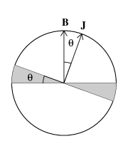
FIG. 1.: Simple representation of weight vectors in the hyper-sphere. The teacher and the student disagree when the input vector S is inside the shaded region.

The intuitive meanings of $\rho$ and of the Eq. 7 can be verified with the help of Fig. 1, observing that $\rho=\cos\theta$ and that for the boolean perceptron the weight vectors are normal to a hyper-plane that divides the hyper-sphere in two differently labelled hemispheres, it is easy to see that the student and the professor disagree on the labeling of input vectors ${\bf S}$ inside the shaded region, thus trivially $e_{G}=\theta/\pi=\frac{1}{\pi}\arccos\rho$ .

B Emergence of the macroscopic dynamics

The dimensionality of the dynamical system involved can be reduced by using (4) and (3) to write a system of coupled difference equations to the macroscopic variables:

$$\rho^{\mu+1} = \rho^{\mu}+\frac{\rho^{\mu}}{N}\left[W^{\mu}({\cal V})\left(\frac{y^{\mu}\tilde{\sigma}^{\mu}_{B}}{\rho^{\mu}}-\Delta^{\mu}\right)-\frac{1}{2}(W^{\mu}({\cal V}))^{2}\right]$$ (8)

$$+ \frac{1}{N}\left[\frac{{\bf J}^{\mu}\cdot{\vec{\eta}}^{\mu}}{J^{\mu}}-\rho^{\mu}\Lambda^{\mu}+\frac{{\bf S}^{\mu}\cdot\vec{\eta}^{\mu}}{N}\tilde{\sigma}^{\mu}_{B}W^{\mu}({\cal V})\right]+{\cal O}\left(\frac{1}{N^{2}}\right)\>,$$ (9)

$$J^{\mu+1} = J^{\mu}+\frac{J^{\mu}}{N}\left(W^{\mu}({\cal V})\Delta^{\mu}+\frac{1}{2}(W^{\mu}({\cal V}))^{2}-\Omega^{\mu}\right)+{\cal O}\left(\frac{1}{N^{2}}\right)\>,$$ (10)

$$B^{\mu+1} = B^{\mu}+\frac{1}{N}\left(\frac{\vec{\eta}^{\mu}\cdot{\bf B}^{\mu}}{B}-\Lambda^{\mu}B^{\mu}\right)+\frac{\vec{\eta}^{\mu}\cdot\vec{\eta}^{\mu}}{2BN^{2}}+{\cal O}\left(\frac{1}{N^{2}}\right)\>.$$ (11)

In the above equations the local stability $\Delta=x\tilde{\sigma}_{B}$ was introduced. Positive stability means that the student classification $\sigma_{J}=sign(x)$ agrees with the (noisy) learning data $\tilde{\sigma}_{B}$.

The usefulness of the TL lies in the possibility of transforming the stochastic difference equations into a closed set of deterministic differential equations [19, 15]. The idea is to choose a continuous time scale $\alpha$ such that for the TL regime $p/N\rightarrow\alpha$, where $p$ is the number of examples already presented. The equations are then averaged over the input vectors $\bf S$ and drift vector $\vec{\eta}$ distributions, leading to:

$$\frac{d\rho}{d\alpha} = \rho\left\langle W\left(\frac{y\tilde{\sigma}_{B}}{\rho}-\Delta\right)-\frac{1}{2}W^{2}\right\rangle+\left\langle\frac{{\bf J}\cdot{\vec{\eta}}}{J}-\rho\Lambda+C_{S\eta}\tilde{\sigma}_{B}W\right\rangle\>,$$ (12)

$$\frac{dJ}{d\alpha} = J\left\langle W\Delta+\frac{1}{2}W^{2}-\Omega\right\rangle\>,$$ (13)

$$\frac{dB}{d\alpha} = \left\langle\frac{\vec{\eta}\cdot{\bf B}}{B}-\Lambda B+C_{\eta\eta}\right\rangle\>,$$ (14)

where $\langle...\rangle=\int d{\vec{\eta}}\>d{\bf S}\,(\ldots)P(\vec{\eta},{\bf S})$ and the definitions $C_{S\eta}=\lim_{N\rightarrow\infty}({\bf S}\cdot{\vec{\eta}})/(NB)$ and $C_{\eta\eta}=\lim_{N\rightarrow\infty}({\vec{\eta}\cdot\vec{\eta}})/(2BN)$ have been used.

The fluctuations in the stochastic equations vanish in the TL and the above equations become exact (self-averaging property). This can be proved by writing the Fokker-Planck equations for the finite $N$ stochastic process defined in (9), (10) and (11), and showing that the diffusive term vanishes in the TL [22].

C Variational optimization of algorithms

The variational approach was proposed in [16] as an analytical method to find learning algorithms with optimal mean decay (per example) of the generalization error. The same method was applied in several architectures and learning situations.

The idea is to write:

$$\frac{de_{G}}{d\alpha}=\frac{\partial e_{G}}{\partial\rho}\frac{d\rho}{d\alpha}\>,$$ (15)

and use equation (12) to build the functional:

$$\frac{de_{G}}{d\alpha}[W]=\frac{\partial e_{G}}{\partial\rho}\left[\rho\left\langle W\left(\frac{y\tilde{\sigma}_{B}}{\rho}-\Delta\right)-\frac{1}{2}W^{2}\right\rangle+\left\langle\frac{{\bf J}\cdot{\vec{\eta}}}{J}-\rho\Lambda+C_{S\eta}\tilde{\sigma}_{B}W\right\rangle\right]\>.$$ (16)

Thus, the optimization is attained by imposing the extremum condition:

$$\frac{\delta}{\delta W({\cal V})}\left(\frac{de_{G}}{d\alpha}[W({\cal V})]\right)_{W=W^{*}}=0\>,$$ (17)

where ${\delta}/{\delta W({\cal V})}$ stands for the functional derivative in the subspace of modulation functions $W$ with dependence in the set $\cal V$. The above equation can be solved observing that $\partial e_{G}/\partial\rho\neq 0$ and

$$\frac{\delta}{\delta W({\cal V})}\langle f({\cal H},{\cal V})W^{n}({\cal V})\rangle=n\langle f({\cal H},{\cal V})\rangle_{\cal H|\cal V}\>W^{n-1}({\cal V})\>,$$ (18)

$f$ is an arbitrary function, $\cal H$ is the set of hidden variables, that is, in contrast with the set ${\cal V}$, the variables not accecible to the student (e.g. fields $y$, drift vector $\vec{\eta}$, etc …) and $\langle...\rangle_{\cal H|\cal V}=\int d{\cal H}P({\cal H}|{\cal V})...$, where for a given set ${\cal H}=\{a_{1},a_{2},..\}$, $d{\cal H}=da_{1}da_{2}...$. The solution is given by:

$$W^{*}({\cal V})=\left\langle\frac{(y+C_{S\eta})\tilde{\sigma}_{B}}{\rho}-\Delta\right\rangle_{{\cal H}|{\cal V}}.$$ (19)

By writing $y+C_{S\eta}=({\bf B}+\vec{\eta})\cdot{\bf S}/\sqrt{B}$ it can be seen that the optimal algorithm “tries” to pull the example stability $\Delta$, not to an estimative of the present teacher stability, but to one already corrected by the effect of the drift $\vec{\eta}$. It seems natural to concentrate on cases where the drift and the input vectors are uncorrelated ($C_{S\eta}=0$).

The optimization under different conditions of information availability, i.e., different specifications of the sets $\cal V$ and $\cal H$, leads to different learning algorithms. This can be seen by performing the appropriate averages in (19), as we proceed to show:

  Annealed Hebb Algorithm:

Suppose that the available information is limited to the corrupted teacher output. This corresponds to the learning situation such that ${\cal H}=\{y,\vec{\eta},|x|,\sigma_{J}\}$ and ${\cal V}=\{\tilde{\sigma}_{B}\}$. Considering that $C_{S\eta}=0$, we need to perform the average:

$$W^{*}(\tilde{\sigma}_{B})=\frac{\tilde{\sigma}_{B}}{\rho}\left\langle y-\rho x\right\rangle_{\{x,y\}|\tilde{\sigma}_{B}},$$ (20)

which involves $\int dy\>y\>P\left(y\mid\tilde{\sigma}_{B}\right);\;\int dx\>x\>P\left(x\mid\tilde{\sigma}_{B}\right).$ The probability distributions are easily obtained using Bayes theorem:

$$P(y\mid\tilde{\sigma}_{B})=\frac{P(\tilde{\sigma}_{B}\mid y)P(y)}{\int dy\>P(\tilde{\sigma}_{B}\mid y)}.$$ (21)

By the Central Limit Theorem we know that, in the TL, $P(y)$ and $P(x)$ are Gaussians with unit variance and it is not difficult to verify, using (1), that :

$$P(\tilde{\sigma}_{B}\mid y)=\frac{\chi}{2}+(1-\chi)\Theta(\tilde{\sigma}_{B}y);\;P(\tilde{\sigma}_{B}\mid x)=\frac{\chi}{2}+(1-\chi)H(-\frac{\tilde{\sigma}_{B}x}{\lambda}),$$ (22)

where $\lambda=\sqrt{1-\rho^{2}}/\rho$ and $H(x)=\int_{x}^{\infty}\frac{dt}{\sqrt{2\pi}}e^{-t^{2}/2}$.

It follows that

$$\left\langle y\right\rangle_{\{x,y\}|\tilde{\sigma}_{B}}=\sqrt{\frac{2}{\pi}}\tilde{\sigma}_{B}(1-\chi);\;\;\;\left\langle\rho x\right\rangle_{\{x,y\}|\tilde{\sigma}_{B}}=\sqrt{\frac{2}{\pi}}\tilde{\sigma}_{B}(1-\chi)\rho^{2}.$$ (23)

Combining the above results in (20) finally gives :

$$W_{AH}(\tilde{\sigma}_{B};\rho,\chi)=\sqrt{\frac{2}{\pi}}\lambda^{2}\rho(1-\chi)\>.$$ (24)

The weight changes are proportional to the Hebb factor, but the modulation function does not depend on the example stability $\Delta$ (see Fig. 2). Hence the name Hebb. However this function is not constant in time, the temporal evolution (annealing) is automatically incorporated into the modulation function. Optimal annealing is achieved by having the modulation function depend on the parameter $\rho$, the normalized overlap between the student ${\bf J}$ and the concept ${\bf B}$. Since this quantity is certainly not available to the student, there will be a need to complement the learning algorithm with an efficient estimator of the present level of performance by the student (see Sec. IV).

FIG. 2.: Modulation functions exemplified for $\rho=0.9$ with noise levels $\chi=0$ (top) and $\chi=0.1$ (bottom): Annealed Hebb (dots), Step (dashes), Symmetric (dashes-dots) and Optimal (solid).

  Step Algorithm ([6]):

This algorithm, obtained under the restriction ${\cal H}=\{y,\vec{\eta},\\ |x|\}$ and ${\cal V}=\{\tilde{\sigma}_{B},\sigma_{J}\}$, is a close relative to Rosemblatt’s original perceptron algorithm, which works by error correcting and treats all the errors in the same manner. There are two important differences, however, since correct answers also cause (smaller) corrections and furthermore, the size of the corrections evolves in time in a similar manner to the annealed Hebb algorithm.

The modulation function is

$$W_{Step}(\tilde{\sigma}_{B},\sigma_{J};\rho,\chi)=\frac{1}{\sqrt{2\pi}}\lambda^{2}\rho(1-\chi)\frac{1}{\left[\frac{\chi}{2}+\frac{(1-\chi)}{\pi}\arccos(-\rho\tilde{\sigma}_{B}\sigma_{J})\right]}\>.$$ (25)

Note that the Step Algorithm has access to the student’s output and can differentiate between right ($\Delta>0$) and wrong ($\Delta<0$) classifications, the name arises from the form of its modulation function (Fig. 2). The annealing increases the height of the step, i.e the difference between right and wrong, as the overlap $\rho$ goes to one.

  Symmetric Weight Algorithm (see [15]):

This is the optimal algorithm for the learning situation described by ${\cal H}=\{y,\vec{\eta},\sigma_{J}\}$ and ${\cal V}=\{\tilde{\sigma}_{B},|x|\}$. The resulting modulation function is given by:

$$W_{SW}(\tilde{\sigma}_{B},|x|;\rho,\chi)=\sqrt{\frac{2}{\pi}}\lambda(1-\chi)e^{-x^{2}/2\lambda^{2}}.$$ (26)

That algorithm cannot discern between wrong and right classifications, but only differentiates between “easy” (large $\mid\Delta\mid$) and “hard” (small $\mid\Delta\mid$) classifications, concentrating the learning in “hard” examples (Fig. 2).

  Optimal Algorithm (see [16, 5, 9]):

When all the available information is used we have the learning situation described by ${\cal H}=\{y,\vec{\eta}\}$ and ${\cal V}=\{\tilde{\sigma}_{B},|x|,\sigma_{J}\}$. the optimal algorithm is then given by:

$$W_{OPT}(\Delta=\tilde{\sigma}_{B}x;\rho,\chi)=\frac{1}{\sqrt{2\pi}}\lambda(1-\chi)\frac{e^{-\Delta^{2}/2\lambda^{2}}}{\chi/2+(1-\chi)H(-\Delta/\lambda)}\;\;.$$ (27)

In the presence of noise, a crossover is built into the Optimal modulation function. This crossover is from a regime where the student classification is not strongly defined ($\Delta$ negative but small) – and the information from the teacher is taken seriously – to a regime where the student is confident on its own answer – and any strong disagreement (very negative $\Delta$) with the teacher will be attributed to noise, and thus effectively disregarded. The scale of the stabilities where the crossover occurs depends on the level of performance $\rho$ and therefore is also annealed.

The learning mechanisms are highly adaptive and remain the same in the case of drifting rules, where the common features described above, mainly the $\rho$ dependent annealing, lead automatically to a forgetting mechanism without the need to impose it, based on heuristic expectations, in an ad hoc manner.

It is interesting to note that the heuristically proposed algorithms are approximations of these optimized modulation functions. For instance, simple Hebb rule is the Annealed Hebb when $\vec{\eta}=0$, since it can be shown in this case that $WJ=1$, and corresponds to the $\rho\rightarrow 0$ regime of all the optimized algorithms; Rosemblatt Perceptron algorithm is qualitatively similar to the Step algorithm; Adatron [2, 32] approximates the Optimal algorithm for $\chi=0$ and $\rho\rightarrow 1$; OLGA [14] and Thermal perceptron [10] algorithms resemble the Optimal modulation with $\chi>0$.

III Learning drifting concepts

The important result from last section is that, under the assumption of uncorrelated drift and input vectors, the modulation functions do not depend on the drift parameters (in contrast with the explicit dependence on the examples noise level $\chi$). So, they are expected to be robust to continuous or abrupt, random or deterministic, concept changes. In this section simple instances of drifting concepts are examined; abrupt changes are studied in Sec. V.

A Random drift

In this scenario, the concept weight vector ${\bf B}$ performs a random walk on the surface of a $N$-dimensional unit sphere. The drift vector has random components with zero mean and variance $2D$,

$$\langle\eta_{i}^{\mu}\eta_{j}^{\nu}\rangle=2D\delta_{ij}\delta_{\mu\nu}\>,$$ (28)

The condition ${\bf B}^{\mu+1}\cdot{\bf B}^{\mu+1}=1$ is imposed in (14) by considering that ${\bf B}^{0}\cdot{\bf B}^{0}=1$ and with the choice $\Lambda=\vec{\eta}\cdot{\bf B}+D.$

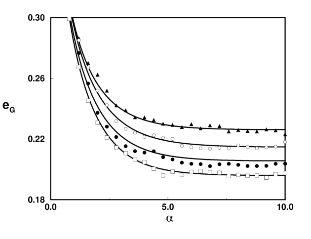
FIG. 3.: Integration of learning equations and simulation results ($N=5000$) for random drift $D=0.1$: Annealed Hebb (triangles), Symmetric (white circles), Step (black circles) and Optimal (white squares). The self-averaging property is clear since the simulation results refer to only one run.

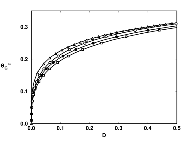
FIG. 4.: Asymptotic error $e_{G}^{\infty}(D)$ for random drift: Annealed Hebb (triangles), Symmetric (white circles), Step (black circles) and Optimal (white squares).

The order of magnitude of the scaling of the drift vector with $N$ is important since it gives the correct time scale for non trivial behavior: if smaller, the drift would be irrelevant in the time scale of learning, while if larger it would not allow any tracking. In the relevant regime, the task in nontrivial also in another sense: the autocorrelation of the concept vector decays exponentially in the $\alpha$-scale, $\langle{\bf B}(\alpha){\bf B}(\alpha^{\prime})\rangle\propto e^{-D(\alpha-\alpha^{\prime})}$.

For the optimized algorithms, the equation for $\rho$ decouples from the equation for $J$. After the proper averages, the learning equation for this type of drift reduces to

$$\frac{d\rho}{d\alpha}=\rho\left\langle W\left(\frac{y\tilde{\sigma}_{B}}{\rho}-\Delta\right)-\frac{1}{2}W^{2}\right\rangle-\rho D\>,$$ (29)

This equation can be solved for each particular modulation function $W$. The generalization error $e_{G}=\frac{1}{\pi}\arccos(\rho)$ for the several algorithms described in the last section are compared in Fig. 3 for the noiseless case. Solid curves refer to integrations of the above learning equation and symbols correspond to simulation results. Although the rule is continuously changing, it can be tracked within an stationary error $e_{G}^{\infty}$ which depends on the drift amplitude $D$. The functions $e_{G}^{\infty}(D)$ for the various algorithms can be found from the condition $d\rho/d\alpha=0$ and are shown in Fig. 4.

TABLE I.: Small drift exponents: Random case

	$e_{G}^{\infty}(D)$	$e_{G}^{\infty}(D=0,\chi=0)$
Annealed Hebb	$\left(\frac{D}{\pi^{3}}\right)^{1/4}\approx 0.42\>D^{1/4}$	$0.40\>\alpha^{-1/2}$
Symmetric	$\left(\frac{\sqrt{2}}{\pi^{2}}\right)^{1/3}D^{1/3}\approx 0.52\>D^{1/3}$	$1.41\>\alpha^{-1}$
Step	$\frac{(4)^{1/3}}{\pi}D^{1/3}\approx 0.51\>D^{1/3}$	$1.27\>\alpha{-1}$
Optimal	$\left(\frac{2}{\pi^{2}A^{2}}\right)^{1/3}D^{1/3}\approx 0.45\>D^{1/3}$	$0.88\>\alpha^{-1}$

This equation can be solved for each particular modulation function $W$. The generalization error $e_{G}=\frac{1}{\pi}\arccos(\rho)$ for the several algorithms described in the last section are compared in Fig. 3 for the noiseless case. Solid curves refer to integrations of the above learning equation and symbols correspond to simulation results. Although the rule is continuously changing, it can be tracked within an stationary error $e_{G}^{\infty}$ which depends on the drift amplitude $D$. The functions $e_{G}^{\infty}(D)$ for the various algorithms can be found from the condition $d\rho/d\alpha=0$ and are shown in Fig. 4. The behavior for small drift is shown in Table 1. Note the abrupt change in the exponents due to the inclusion of more information than the output $\tilde{\sigma}_{B}$. The behavior for small drift is shown in the Table 1. Note the abrupt change in the behavior due to the inclusion of more information than the output $\tilde{\sigma}_{B}$.

B Deterministic drift

In the learning scenario considered so far, the worst case drift will occur when at each time step the concept is changed deterministically so that the overlap with the current student vector is minimized. In this situation, previously examined by Biehl and Schwarze [4], the new concept is chosen by minimizing ${\bf B}^{\mu+1}\cdot{\bf J}^{\mu}$ subject to the conditions

$${\bf B}^{\mu+1}\cdot{\bf B}^{\mu} = 1-\frac{D}{N^{2}}\>,$$ (30)

$${\bf B}^{\mu+1}\cdot{\bf B}^{\mu+1} = 1\>,$$ (31)

where now $D$ is the drift amplitude for the deterministic case. Note the different scaling with $N$ for non trivial behavior.

TABLE II.: Small drift exponents: Deterministic case

	$e_{G}^{\infty}(D)$	$e_{G}^{\infty}(D=0,\chi=0)$
Annealed Hebb	$\left(\frac{\sqrt{2D}}{\pi^{2}}\right)^{1/3}\approx 0.52\>D^{1/6}$	$0.40\>\alpha^{-1/2}$
Symmetric	$\left(\frac{4D}{\pi^{2}}\right)^{1/4}\approx 0.80\>D^{1/4}$	$1.41\>\alpha^{-1}$
Step	$\frac{2^{5/4}}{\pi}D^{1/4}\approx 0.76\>D^{1/4}$	$1.27\>\alpha^{-1}$
Optimal	$\left(\frac{8D}{A^{2}}\right)^{1/4}\approx 0.63\>D^{1/4}$	$0.88\>\alpha^{-1}$

Clearly ${\bf B}^{\mu+1}$ lies in the same plane which contains ${\bf B}^{\mu}$ and ${\bf J}^{\mu}$. The solution of this constrained minimization problem is

$${\bf B}^{\mu+1} = a{\bf B}^{\mu}-b{\bf J}^{\mu}\>,$$ (32)

$$a = 1-\frac{D}{N^{2}}+bJ\rho,$$ (33)

$$b = \frac{1}{JN}\left[\frac{2D-(D/N)^{2}}{1-\rho^{2}}\right]^{1/2}\>.$$ (34)

In terms of $\Lambda$ and $\vec{\eta}$ of eq. 4 is

$$\Lambda=(1-a)N\>,\>\>\>\>\vec{\eta}=-b{\bf J}N\>.$$ (35)

The learning equation reduces to

$$\frac{d\rho}{d\alpha}=\rho\left\langle W\left(\frac{y\tilde{\sigma}_{B}}{\rho}-\Delta\right)-\frac{1}{2}W^{2}\right\rangle-\sqrt{2D(1-\rho^{2})}\>,$$ (36)

and the analysis is similar to the previous subsection. Theoretical error curves confirmed by simulations are shown in Fig. 5 for the different algorithms with fixed drift amplitude. The stationary tracking error $e_{G}^{\infty}(D)$ is shown in Fig. 6.

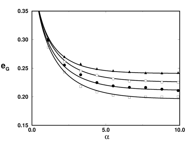
FIG. 5.: Integration of learning equations and simulation results ($N=5000$) for deterministic drift $D=0.01$: Annealed Hebb (triangles), Symmetric (white circles), Step (black circles) and Optimal (white squares).

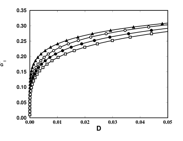
FIG. 6.: Asymptotic error $e_{G}^{\infty}(D)$ for deterministic drift: Annealed Hebb (triangles), Symmetric (white circles), Step (black circles) and Optimal (white squares).

The behavior for small drift $D$ is shown in Table II. Again we can note the occurrence of an abrupt change in the exponents after the inclusion of information on the student’s fields.

C Asymptotic behavior: Critical exponents and universality classes for unlearnable problems

A simple, although partial, measure of the performance of a learning algorithm can be given by the asymptotic decay of the generalization error in the driftless case and alternatively by the residual error dependence on $D$ in the presence of drift. These are not independent aspects, but rather linked in a manner reminiscent of the relations between the different exponents that describe power law behavior in Critical Phenomena.

In the absence of concept drift, the generalization error decays to zero when $\alpha$ approaches $\alpha_{c}$ (which here happens to be infinity but may have a finite value in other situations [32]) as a power law of the number of examples with the so called learning or static exponent $\beta$,

$$e_{G}\propto\tau^{\beta}\>,$$ (37)

where $\tau\equiv\frac{1}{\alpha}-\frac{1}{\alpha_{c}}$. Thus, we may think of $e_{G}$ as a kind of order parameter in the sense that it is a quantity which changes from zero to a finite value at $\tau=0$. We may think of $1/\alpha$ as the analogous of the control parameter $T$ (temperature) in critical phenomena.

Any amount of drift in the concept, changes the problem from a learnable to an unlearnable one, with a residual error $e_{G}^{\infty}\equiv e_{G}(\tau=0)$. We have seen that this behavior at the critical point $\tau=0$ also obeys a power law

$$e_{G}^{\infty}\propto D^{1/\delta}\>,$$ (38)

where $\delta$ has been called the drift exponent.

In principle, we can classify different unlearnable situations (due to say, various kinds of concept drift), by the two exponents $\beta$ and $\delta$. Different algorithms and learning situations may have the same exponents. We can thus define, in a spirit similar to that in the study of Critical Phenomena the so called universality classes of behavior. In this paper we have seen four classes of behavior $(\beta,\delta)$, the combinations $(1/2,4),(1,3)$ for the random drift case and $(1,4),(1/2,6)$ for the deterministic case. In the absence of drift $\beta=1$ for the Hebb algorithm, and $\beta=1$ for the symmetric, step and optimal algorithms we have introduced above. There exist, however, other classes. For example, for the standard Rosemblatt Perceptron algorithm with fixed learning rate we have $\beta=1/3$; then, $\delta=5$ for random drift and $\delta=8$ for deterministic drift.

We have observed that, in general, the two exponents are independent. However, if a simple condition holds, then there exists a relation connecting $\beta$ and $\delta$ for each kind of drift. For example, as can be compared with the above results,

$$\delta = \frac{1}{\beta}+2\>,\>\>\>\>\mbox{(random drift)}$$ (39)

$$\delta = \frac{2}{\beta}+2\>,\>\>\>\>\mbox{(deterministic drift)}\>.$$ (40)

To derive these relations we remember that $e_{G}\propto\sqrt{1-\rho^{2}}$ when $\rho\rightarrow 1$, so that we may write in this limit the learning equation as

$$\frac{de_{G}}{d\alpha}\approx CD^{m}e_{G}^{-n}-C_{1}(D)e_{G}^{n_{1}}-C_{2}(D)e_{G}^{n_{2}}-\ldots\>,$$ (41)

where $C$ is a constant, $C_{k}(D)$ are functions of $D$ and $n$ and $n_{k}$ are positive numbers. Now, denote by $C_{*}(D)$ the first function which survives in the limit $D\rightarrow 0$, $C_{*}(D\rightarrow 0)=C_{*}$. Then, the learning equation is

$$\frac{de_{g}}{d\alpha} \approx -C_{*}e_{G}^{n_{*}}\>,$$ (42)

$$e_{G}(\alpha) \approx \left(C_{*}(n_{*}-1)\alpha\right)^{-1/(n_{*}-1)}\>\>\>\>(n_{*}>1)\>,$$ (43)

$$e_{G}(\alpha) \propto e^{-C_{*}\alpha}\>\>\>\>(n_{*}=1)\>.$$ (44)

Thus,

$$\beta=1/(n_{*}-1)\>,$$ (45)

with $\beta\rightarrow\infty$ denoting exponential decay.

In the presence of small drift, we may write $C_{1}(D)\propto D^{m_{1}}$. The stationary condition $de_{G}/d\alpha=0$ leads to

$$e_{G}^{\infty}(D)\approx D^{\frac{m-m_{1}}{n_{1}+n}}\>,$$ (46)

$$\delta=\frac{n_{1}+n}{m-m_{1}}\>.$$ (47)

This shows that, in principle, the two exponents are independent. However, if happens that the first surviving function is $C_{*}(D)=C_{1}(D)$ (which seems to be a very common situation), then $n_{*}=n_{1}$ and $m_{1}=0$, so that

$$\delta=\frac{1}{m}\left(\frac{1}{\beta}+(1+n)\right)\>.$$ (48)

The relations given by Eq. (39) follow from the fact that $n=1,m=1$ for random drift and $n=0$ and $m=1/2$ for deterministic drift. Other drift scenarios may define other universality classes.

In the case where $C_{*}\neq C_{1}$, we only can conclude that

$$\delta>\frac{1}{m}\left(\frac{1}{\beta}+(1+n)\right)\>.$$ (49)

It is important to note an exponential decay of the error $(\beta=\infty)$ leads to the limiting value $\delta=2$ both for deterministic as random drift. It is know that the error cannot decay faster than exponential in these learning problems.

IV Practical considerations

The most important question that can be raised in the implementation of the variational ideas as a guide to construct algorithms is how to measure the several unavailable quantities that go into the construction of the modulation function. The problem of inferring the example distribution will not be considered and only a simple method to measure the student-teacher overlap $\rho$ will be presented. This is done by adding a ‘module’ to the perceptron in order to estimate online the generalization error, as studied in [17]. Algorithms that rely on this kind of module are quite robust with respect to changes in the distribution of examples and even to lack of statistical independence [20]. Consider an online estimator (a ‘running average’) which uses the instantaneous error $\epsilon^{\mu}=(1-\sigma_{B}^{\mu}\sigma_{J}^{\mu})/2$ to update the current estimate of the generalization error:

$$\hat{e}_{G}^{(\mu+1)}=(1-\frac{\omega}{N})\hat{e}_{G}^{(\mu)}+\frac{\omega}{N}\epsilon^{\mu}\>.$$ (50)

This estimator incorporates exponential memory loss through the $\omega$ parameter. In the perceptron, due to the factor $\lambda=\tan(\pi e_{G})$ that appears in the modulation function, fluctuations around $e_{G}\approx\frac{1}{2}$ may lead to spurious divergences. Therefore it is natural to consider the truncated Taylor expansion

$$\hat{\lambda}_{k}=\tan^{(k)}(\pi\hat{e}_{G})=\pi\hat{e}_{G}+\frac{1}{3}(\pi\hat{e}_{G})^{3}+\frac{2}{15}(\pi\hat{e}_{G})^{5}+\cdot\cdot\cdot+c_{k}(\pi\hat{e}_{G})^{k}\>.$$ (51)

Then, the modulation function for an adaptive algorithm inspired in the noiseless optimal algorithm is

$$W(\hat{\lambda}_{k},\Delta_{\mu})=\frac{1}{\sqrt{2\pi}}\frac{\hat{\lambda}_{k}}{H(\frac{-\Delta_{\mu}}{\hat{\lambda}_{k}})}\exp(-\frac{\Delta_{\mu}^{2}}{2\hat{\lambda}_{k}^{2}})\>.$$ (52)

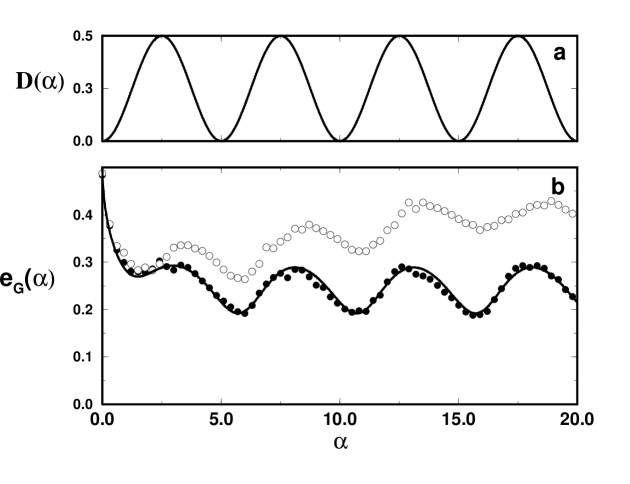
FIG. 7.: a) Oscillating drift level $D=D_{0}\sin^{2}(2\pi\nu t)$ for $D_{0}=0.5,\nu=0.1$. b) Integration of the differential equation for the oscillating case $D_{0}=0.5,\nu=0.1$ (thick solid). Adaptive optimal algorithm with $\omega=2$ and $k=3$ (black circles) and simple Hebb algorithm (white circles)

In figure 7 we present the results of applying this algorithm to a problem where the drift itself is non-stationary. We have dubbed this non-stationarity drift acceleration. The algorithm is quite uninterested in the particular type of drift acceleration, and as an illustration we chose a drift given by $D=D_{0}\sin^{2}(2\pi\nu t)$. The adaptive algorithm makes no use of this knowledge. There has been no attempt at optimizing the estimator itself, but a reasonable and robust choice is $\omega=2$ and $k=3$. Simulations were done for $N=1000$, a size regime, where for all practical purposes, the central limit theorem holds. Note that the Hebb algorithm is not able to keep track of the rule since it has no internal forgetting mechanism.

We have not studied the mixed case of drift in the presence of noise. The nature of the noise process corrupting the data is essential in determining the asymptotic learning exponent ($\beta$). While multiplicative (flip) noise does not alter $\beta$ for the optimized algorithms, additive (weight) noise does. This extension deserves a separate study. See [5] for the behavior of the optimized algorithm and noise level estimation in the presence of noise acceleration in the absence of drift, see also [12] where it is shown that learning is possible even in the mixed drift-noise case.

V The Wisconsin test for perceptrons: Piecewise constant rules

How do the algorithms studied in the previous sections perform in the case of abrupt changes (piecewise constant rules)? The interest is in determining how do the optimal algorithms fare in a task for which they were not optimized. The Wisconsin test (WT) for perceptrons (WTP) to be studied here was inspired in what is called the WT and is used in the diagnostics of pre-frontal lobe (PFL) syndrome in human patients and which will now be described very briefly (for details see e.g. [27, 21]).

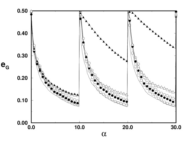
FIG. 8.: Simulations for $N=500$ in single runs. Bottom line: lower bound given by the Optimal algorithm with the true values of $\lambda$. Symbols: Optimal algorithm (white squares), Step algorithm (black circles), Symmetric Weight algorithm (white circles), Annealed Hebb (white triangles), all with $\omega=2$ and $k=3$ estimator and and Hebb (black triangles).

Consider a deck of cards, each one has a set of pictures. The cards can be arranged in several different manners into two categories. The different possible classifications can be done according, e.g. to color (black or red pictures), to parity (even or odd number of figures in the picture), to sharpness (figures can be round or pointed) etc. The examiner chooses a rule and a patient is shown a sequence of cards and asked to classify them. The information, whether the patient presumed classification is correct or not, is made available before the next presentation. After a few trials (5-10) normal subjects are able to infer the desired rule. PFL patients are reported to infer correctly the rule after as little as 15 trials. Now a new rule is chosen at random by the examiner but the patient is not informed about the change. Normal patients are quick to pick up the change and after a small number of trials (5-10) are again able to correctly classify the cards. PFL patients are reported to persevere in the old rule and after as much as 60 trials still insist in the old classification rule.

Our WTP is designed as a direct implementation of these ideas, by considering learning of a piecewise constant teacher, without resetting the couplings to tabula rasa, i.e, without letting the patient know that the rule has changed.

Fig. (8) shows the results of simulations with the adaptive algorithm of (52). The rule is constant up to $\alpha=10$, it then suddenly jumps to another, uncorrelated vector and stays again unchanged until $\alpha=20$ and so on. The most striking feature is that the perceptron with pure Hebbian algorithm works quite efficiently for the first rule but perseveres in that state and adapts poorly to a change. It can not detect performance degradation and is not surprised by the errors. The reason for that is that the scale of the weight changes is the same independently of the length of the ${\bf J}$ vector. The other algorithms are able to adapt to the new conditions in as much as they incorporate the estimate of the performance of the student.

VI Conclusions

The necessary ingredients for the online tracking of drifting concepts, adaptation to non-stationary noise etc., emerge naturally and in an integrated way in the optimized algorithms. These ingredients have been theoretically derived rather than heuristically introduced. Many of the current ideas in machine learning of changing concepts can be viewed as playing a role similar to the ideal features discussed here for the perceptron. Among the important ideas arising from the variational approach are:

• Learning algorithms from first principles: For each one of these simple learning scenarios an ideal and optimal learning algorithm can be found from first principles. These optimized algorithms do not have arbitrary parameters like learning rates, acceptance thresholds, parameters of learning schedules, forgetting factors etc. Instead, they have a set of features which play similar roles to those heuristic procedures. The exact form of these features may suggest new mechanisms for better learning.

• Learn to learn in changing environments: The Optimal modulation function $W$ indeed represents a parametric family of functions, the (non-free) parameters being the same as those present in the probability distribution of the learning problem: $J$, $\rho$, $\chi$, etc. The modulation function changes during learning, that is, the algorithm moves in this parametric space during the learning process. The student “learns to learn” by online estimation of the necessary parameters of its modulation function.

• Robustness of optimized algorithms: Historically, a multitude of learning algorithms has been suggested for the perceptron: Rosemblatt’s Perceptron, Adaline, Hebb, Adatron, Thermal Perceptron, OLGA, etc. From the variational perspective, these practical algorithms can be viewed as more or less reliable approximations of the ideal ones in the TL. For example, simple Hebb corresponds to the Optimal algorithm in the limit $\rho\rightarrow 0$; Adatron (Relaxation) algorithm is related to the limit $\rho\rightarrow 1$; OLGA [14] and Thermal perceptron [10] includes an acceptance threshold which mimics the optimal algorithm in the presence of multiplicative noise $\chi$. Thus, although the optimal algorithms are derived for very specific distributions of examples, it does not mean that they are fragile, non-robust when applied in other environments. They are indeed very robust [20], at least for the environments in which the standard algorithms work, since these practical algorithms are ‘particular cases’ of a more general modulation function. But since new learning situations (new types of noise, drifting processes, general non-stationarity etc.) can be theoretically examined from the variational viewpoint, it is possible that new features emerge, and that these suggest new practical ideas for more robust and efficient learning.

• Emergence of ‘cognitive’ modules: Have the variational ideas any relevance to ‘Biological Machine Learning’? Probably not for the biological structures, which are produced by opportunistic ‘evolution bricolage’, but perhaps they might apply in understanding biological cognitive functions. The variational approach brings forth a suggestion that, even if not new, acquires a more concrete form due to the transparent nature of the simple models studied: optimization of the learning ability leads to the emergence of ‘cognitive functional modules’, here defined as components of the modulation function and accessory estimators of relevant quantities of the probability distribution related to the learning situation. A tentative list of such estimators suggested by the variational approach may be: a) a mismatch (surprise) module for detection of discrepant examples; b) an emotional/attentional module for providing differential memory weight for these discrepant examples; c) ‘constructivist’ filters which accommodate or downplay the highly discrepant data; d) noise level estimators for tuning these filters; e) a working memory system for online estimation of current performance which enables detection of environmental changes. In conclusion, the variational approach suggests that the necessity of certain cognitive functions may be related to statistical inference principles already present in simple learning machines.

• Extensions: All the results here presented have been obtained under a rather severe set of restrictions from a practical point of view. The main points concern the TL; noise, order parameter and example distribution estimation; larger architecture complexity. At present we don’t know how to handle finite size effects. That the parameter estimation problem is probably easier than the others is suggested by the robustness found in [8]. The extension of the variational program to architectures experimentally more relevant, specially to include hidden nodes and soft transfer functions [31, 25] has shown that this is a difficult task. The effects that drift may have are not known, but it could even induce faster breaking of the permutation symmetry among the hidden nodes, thus affecting the plateaus structure.

Important remaining questions concern whether the variational approach can be successfully applied to other learning models (radial basis functions, mixture models etc.). The answers will help in determining the difference between universal and particular features of the learning systems.

Acknowledgments: OK and RV were supported by FAPESP fellowships. NC was partially supported by CNPq and FINEP/RECOPE.

REFERENCES

- [1] Amari, S. (1967). Theory of adaptive pattern classifiers. IEEE Transactions, EC-16, 299–307.
- [2] Anlauf, J.K. and Biehl, M. (1989). The AdaTron: an adaptive perceptron algorithm. Europhysics Letters, 10, 687–692.
- [3] Biehl, M. and Schwarze, H. (1992). Online learning of a time-dependent rule. Europhysics Letters, 20, 733–738.
- [4] Biehl, M. and Schwarze, H. (1993). Learning drifting concepts with neural networks. Journal of Physics A.: Mathematical and General, 26, 2651–2665.
- [5] Biehl, M., Riegler, P. and Stechert, M. (1995). Learning from noisy data: an exactly solvable model. Physical Review E 52, R4624–R4627.
- [6] Copelli, M. (1997). Noise robustness in the perceptron. Proceedings of the ESANN’97. (Belgium).
- [7] Copelli, M. and Caticha, N. (1995). Online learning in the committee machine. Journal of Physics A: Mathematical and General, 28, 1615–1625.
- [8] Copelli, M., Eichhorn, R., Kinouchi, O., Biehl, M.; Simonetti, R., Riegler, P. and Caticha, N. (1996) Noise Robustness in Multilayer Neural Networks Europhysics Letters 37 427
- [9] Copelli, M., Kinouchi, O. and Caticha, N. (1996). Equivalence between learning in noisy perceptrons and tree committee machines. Physical Review E 53, 6341–6352.
- [10] Frean, M. (1992). A ‘thermal’ perceptron learning rule. Neural Computation 4, 946–957.
- [11] Haussler, D., Kearns, M., Seung, H. S. and Tishby, N. (1996). Rigorous learning curve bounds from Statistical Mechanics. Machine Learning Journal 25, 195–236.
- [12] Heskes, T. (1994). The use of being stubborn and introspective, In J. Dean, H. Cruse and H. Ritter (Eds.) Proceedings of the ZiF Conference on Adaptive Behavior and Learning . University of Bielefeld, Bielefeld, Germany.
- [13] Hondou, T. (1996). Self-Annealing Dynamics in a Multistable System. Progress in Theoretical Physics, 95, 817–822.
- [14] Kim, J.W. and Sompolinsky, H. (1996). Online Gibbs learning. Physical Review Letters, 76, 3021–3024.
- [15] Kinouchi, O. and Caticha, N. (1992). Biased learning in Boolean Perceptrons. Physica A, 185, 411–416.
- [16] Kinouchi, O. and Caticha, N. (1992). Optimal generalization in perceptrons. Journal of Physics A: Mathematical and General, 25, 6243–6250.
- [17] Kinouchi, O. and Caticha, N. (1993). Lower bounds on generalization errors for drifting rules. Journal of Physics A: Mathematical and General,26, 6161–6171.
- [18] Kinouchi, O. and Caticha, N. (1995). Online versus offline learning in the linear perceptron: A comparative study. Physical Review E, 52, 2878–2886.
- [19] Kinzel, W. and Ruján, P. (1990). Inproving a network generalization ability by selecting examples. Europhysics Letters, 13, 473–477.
- [20] Kuva, S., Kinouchi, O., and Caticha, N. (in press). Learning a spin glass: determining Hamiltonians from metastable states. Physica A.
- [21] Levine, D. S., Leven, S. J. and Prueit, P. S.(1992). Integration, disintegration, and the frontal lobes. In Levine, D.S. and Leven, S.J. (Eds.), Motivation, Emotion and Goal Direction in Neural Networks. Hillsdale, NJ: Erlbaum.
- [22] Mace, C.W.H. and Coolen, A.C.C. (in press). Statistical mechanical analysis of the dynamics of learning in perceptrons. Statistics and Computing.
- [23] Opper, M. and Kinzel, W. (1996). Statistical mechanics of generalization. In van Hemmen,J.L., Domany E. and Schulten K. (Eds.), Physics of Neural Networks. Berlin: Springer.
- [24] Opper, M. (1996). Online versus offline learning from random examples: general results. Physical Review Letters, 77, 4671–4674.
- [25] Rattray, M. and Saad, D. (1997). Globally optimal online learning rules for multi-layer neural networks. Journal of Physics A: Mathematical and General, L771–776.
- [26] Seung, H.S., Sompolinsky, H. and Tishby, N. (1992). Statistical mechanics of learning from examples. Physical Review A, 45, 6056–6091.
- [27] Shallice, T. (1988). From Neuropsychology to Mental Structures. Cambridge: Cambridge University Press.
- [28] Simonetti, R. and Caticha, N. (1996). Online learning in parity machines. Journal of Physics A: Mathematical and General, 29, 4859–4867.
- [29] Valiant, L.G. (1984). A Theory of the Learnable Communications of ACM 27, 1134– 1142.
- [30] Van den Broeck, C. and Reimann P. (1996) Unsupervised learning by examples: online versus offline. Physical Review Letters, 76, 2188–2191.
- [31] Vicente, R. and Caticha, N. (1997). Functional optimization of online algorithms in multilayer neural networks. Journal of Physics A: Mathematical and General, 30, L599–L605.
- [32] Watkin , T.L.H., Rau, A. and Biehl, M. (1993). The statistical mechanics of learning a rule. Reviews of Modern Physics, 65, 499–556.