DTP-97-63

SPhT-98/007

NBI-HE-97-63

Abstract

Consider a random three-coordinate lattice of spherical topology having $2v$ vertices and being densely covered by a single closed, self-avoiding walk, i.e. being equipped with a Hamiltonian cycle. We determine the number of such objects as a function of $v$. Furthermore we express the partition function of the corresponding statistical model as an elliptic integral.

PACS codes: 05.20.y, 04.60.Nc, 02.10.Eb
Keywords: Hamiltonian cycle, self-avoiding walk, random lattice, $O(n)$ model

1 Introduction

Hamiltonian cycles play an important role in the study of the configurational statistics of polymers [1]. Given a lattice, a Hamiltonian cycle is defined as a closed, self-avoiding walk which visits each vertex of the lattice once and only once. Typically, in polymer physics, one has been interested in calculating the number of Hamiltonian cycles for a lattice with a certain regular structure and a given number of vertices. This counting problem has been exactly solved only in a few cases, namely for the two-dimensional Manhattan oriented square lattice [2], the two-dimensional ice lattice [3] and the two-dimensional hexagonal lattice [4, 5]. A field theoretical approach to the problem of counting Hamiltonian cycles on regular lattices was invented by H. Orland et. al. [6] and has recently been further developed by S. Higuchi [7].

Here we address the problem of counting Hamiltonian cycles on random lattices. Whereas on a regular lattice the choice of boundary conditions has to be carefully considered and plays a crucial role for the outcome of the analysis (see for instance [1] for a discussion) on a random lattice no such complications occur. Furthermore one might speculate if the complex dynamics of polymers does not call for a random lattice rather than a regular one.

Consider a random three-coordinate lattice of spherical topology having $2v$ vertices and being equipped with a Hamiltonian cycle. In the present paper we aim at determining the number of such objects as a function of $v$. The objects in question can also be viewed as spherical triangulations consisting of $2v$ triangles and being densely covered by a single closed, self-avoiding walk (where it is understood that the walk consists of links belonging to the dual lattice). Not any three-coordinate graph has a Hamiltonian cycle. Obviously, one-particle-reducible graphs do not, but there also exist one-particle-irreducible graphs which can not be equipped with a Hamiltonian cycle. We show an example of such a graph along with the corresponding triangulation in figure 1.

Figure 1: A three-coordinate one-particle-irreducible graph, which does not have a Hamiltonian cycle (a), and the corresponding triangulation (b) or equivalently (c).

In order to study the above mentioned combinatorial problem we consider a matrix model which generates graphs or triangulations of the relevant type, namely the $n\rightarrow 0$ limit of the fully packed $O(n)$ model on a random lattice. The $O(n)$ model is a so-called loop-gas model and the loops, being closed, self-avoiding and non-intersecting play the role of the walks. In the fully packed model all vertices of the generated graphs are visited by a loop and in the limit $n\rightarrow 0$ only one loop remains. The regular lattice version of the fully packed $O(n)$ model was studied in references [4, 8, 5, 9].

The $O(n)$ model on a random lattice comes in two different versions, an unrestricted one [10, 11] and a restricted one [12]. In the latter the loops are restricted to having even length while in the former there is no restriction on the loop length. On a regular lattice all loops necessarily have even length. The two different versions of the random lattice $O(n)$ model have different critical properties. The restricted $O(n)$ model belongs to the universality class of the unrestricted $O(\frac{n}{2})$ model [12]. The fully packed, restricted $O(n)$ model with $n=2$ is of particular interest because it describes the generalisation of Baxter’s three-colour problem [13] to a random lattice [14, 12]. As long as one considers triangulations consisting only of an even number of triangles (such as those corresponding to a two-dimensional manifold without boundaries) the $n\rightarrow 0$ limit of the fully packed, unrestricted $O(n)$ model coincides with the $n\rightarrow 0$ limit of the fully packed, restricted $O(n)$ model. Since the unrestricted $O(n)$ model on a random lattice is mathematically easier to handle than the restricted one, we shall take as our starting point the unrestricted one. We note, however, that our $n\rightarrow 0$ solution applies to the restricted model as well.

2 The Model

Our starting point is the following matrix model

$$Z(g)=\int_{N\times N}dA\prod_{i=1}^{n}dB_{i}\exp\left\{-N{\,\rm Tr}\>\left[\frac{1}{2}A^{2}+\frac{1}{2}\sum_{i=1}^{n}B_{i}^{2}-\sqrt{g}\sum_{i=1}^{n}AB_{i}^{2}\right]\right\}$$ (2.1)

where $A$ and $B_{i}$ are hermitian $N\times N$ matrices. This matrix model generates triangulations which are densely covered by closed, self-avoiding and non-intersecting loops which come in $n$ different colours. More precisely we can write the free energy $F(g)=\frac{1}{N^{2}}\log Z(g)$ as

$$F(g) = \sum_{h=0}^{\infty}N^{-2h}F_{h}(g),$$

$$F_{h}(g) = \sum_{v=1}^{\infty}{\cal N}_{h}(2v)\,g^{v},\hskip 28.45274pt{\cal N}_{h}(2v)=\sum_{i=0}^{v}n^{i}{\cal N}_{h}^{(i)}(2v).$$ (2.2)

The quantity ${\cal N}_{h}^{(i)}(2v)$ counts the number of genus $h$ triangulations built from $2v$ triangles and densely covered by $i$ closed, self-avoiding and non-intersecting loops . In the following we shall aim at determining ${\cal N}_{0}^{(1)}(2v)$, i.e. the number of spherical triangulations consisting of $2v$ triangles and being densely covered by a single closed, self-avoiding walk. First, let us write instead of (2.1)

$${\cal Z}(g) = \left(\sqrt{g}\right)^{N^{2}}Z(g)$$ (2.3)

$$= \int_{N\times N}dA\prod_{i=1}^{n}dB_{i}\exp\left\{-N{\,\rm Tr}\>\left[\frac{1}{2g}A^{2}+\frac{1}{2}\sum_{i=1}^{n}B_{i}^{2}-\sum_{i=1}^{n}AB_{i}^{2}\right]\right\}.$$

Furthermore, let us introduce a resolvant $W(z)$ corresponding to the model given by the partition function ${\cal Z}(g)$

$$W(z)=\langle\frac{1}{N}{\,\rm Tr}\>\frac{1}{z-A}\rangle=\sum_{h=0}^{\infty}N^{-2h}\,W_{h}(z).$$ (2.4)

We shall be interested only in the large-$N$ limit of the resolvant, $W_{0}(z)$

$$W_{0}(z){\mathop{\sim}_{z\to\infty}}\,\,\,\,\sum_{m=0}^{\infty}\frac{t_{m}}{z^{m+1}},\hskip 19.91684ptt_{m}=\langle\frac{1}{N}{\,\rm Tr}\>A^{m}\rangle_{h=0}.$$ (2.5)

Let us consider the quantity $t_{2}$

$$t_{2} = \frac{2g^{2}}{N^{2}}\frac{d}{dg}\log\left\{(\sqrt{g})^{N^{2}}Z(g)\right\}_{h=0}=g+2g^{2}\frac{d}{dg}F_{0}(g)$$ (2.6)

$$= g+2\sum_{v=0}^{\infty}\sum_{i=0}^{v}n^{i}{\cal N}_{0}^{(i)}(2v)\,v\,g^{v+1}.$$

We see that we can achieve our aim of calculating ${\cal N}_{0}^{(1)}(2v)$ by determining the contribution to $t_{2}$ which depends linearly on $n$. In order to do so, we shall make use of the well-known loop equation for the resolvant [10, 11]. This equation can be derived by making use of the invariance of the matrix integral (2.3) under analytic redefinitions of the fields and reads in the large-$N$ (spherical) limit

$$\frac{1}{g}\left(zW(z)+(1-z)W(1-z)-2\right)=\left(W(z)\right)^{2}+\left(W(1-z)\right)^{2}+nW(z)W(1-z)$$ (2.7)

We now introduce the following functions

$$\xi_{m}(z) = \frac{1}{z^{m}}+\frac{1}{(1-z)^{m}},$$

$$\xi_{m,p}(z) = \frac{1}{z^{m}(1-z)^{p}}+\frac{1}{(1-z)^{m}z^{p}}.$$ (2.8)

The functions $\xi_{m,p}(z)$ can be expressed in terms of the $\xi_{k}(z)$ as follows

$$\xi_{m,p}(z)=\sum_{k=1}^{m}\left(\begin{array}[]{c}m+p-1-k\\ p-1\end{array}\right)\xi_{k}(z)+\sum_{k=1}^{p}\left(\begin{array}[]{c}m+p-1-k\\ m-1\end{array}\right)\xi_{k}(z)$$ (2.9)

and in terms of the $\xi$-functions we can write the loop equation (2.7) as

$$\frac{1}{g}\sum_{l=1}^{\infty}t_{l}\xi_{l}=\sum_{k,l}t_{k}t_{l}\xi_{k+l+2}+\frac{n}{2}\sum_{k,l=0}^{\infty}\xi_{k+1,l+1}t_{k}t_{l}.$$ (2.10)

Using the relation (2.9) and identifying the coefficients of each $\xi_{m}$ in (2.10) we get for $m\geq 2$

$$\frac{1}{g}t_{m}=\sum_{k=0}^{m-2}t_{k}t_{m-k-2}+n\sum_{l,k=0}^{\infty}t_{m+k-1}t_{l}\left(\begin{array}[]{c}k+l\\ l\end{array}\right).$$ (2.11)

This equation can be solved perturbatively in $n$ and $g$. First, let us set $t_{m}=g^{m/2}T_{m}$. Then we have

$$T_{m}=\sum_{k=0}^{m-2}T_{k}T_{m-k-2}+n\sum_{v=1}^{\infty}\sum_{k=1}^{v}\left(\begin{array}[]{c}v-1\\ k-1\end{array}\right)T_{v-k}T_{m+k-2}\,g^{v/2}$$ (2.12)

From this we see that the $T_{k}$’s have the following expansion

$$T_{k}=\sum_{v=0}^{\infty}\sum_{i=0}^{v}n^{i}\,T_{k}^{(i,v)}g^{v/2}$$ (2.13)

and that

$$2v\,{\cal N}_{0}^{(1)}(2v)=\,T_{2}^{(1,2v)}.$$ (2.14)

3 Exact solution as $n\rightarrow 0$

For $n=0$ our model (2.3) is nothing but the Gaussian one-matrix model and we have

$$T_{2k}^{(0,0)}=c_{k}\equiv\frac{(2k)!}{k!(k+1)!},\hskip 19.91684ptT_{2k+1}^{(0,0)}=0.$$ (3.1)

Here $c_{k}$ is the Catalan number of order $k$ which counts in particular the number of distinct configurations of $k$ non-intersecting arches drawn on top of a line.

Equating the terms linear in $n$ in equation (2.12) we see that

$$T_{2}^{(1,2v)} = 2v\,{\cal N}_{0}^{(1)}(2v)=\sum_{k=1}^{v}\left(\begin{array}[]{c}2v-1\\ 2k-1\end{array}\right)T_{2k}^{(0,0)}\,T_{2v-2k}^{(0,0)}$$ (3.4)

$$= \frac{2(2v-1)!}{(v+2)!(v-1)!}\sum_{k=1}^{v}\left(\begin{array}[]{c}v+2\\ k+1\end{array}\right)\left(\begin{array}[]{c}v-1\\ k-1\end{array}\right)$$ (3.9)

$$= \frac{2(2v-1)!(2v+1)!}{(v+2)!(v+1)!\,v!\,(v-1)!}.$$ (3.10)

To prove the last equality one can for instance compare the terms of power zero in $x$ on the two sides of the obvious identity

$$\frac{1}{x}\,\left(1+x\right)^{v+2}\,\frac{1}{x}\left(1+\frac{1}{x}\right)^{v-1}=\frac{1}{x^{v+1}}\left(1+x\right)^{2v+1}.$$ (3.11)

Next, let us define a partition function for spherical triangulations densely covered by a single closed and self-avoiding walk

$$F_{0}^{(1)}(g) \equiv \sum_{v=1}^{\infty}{\cal N}_{0}^{(1)}(2v)\,g^{v}$$ (3.12)

$$= \sum_{v=1}^{\infty}\frac{(2v-1)!(2v+1)!}{(v+2)!(v+1)!(v!)^{2}}\,g^{v}$$

$$= \frac{1}{2g^{2}}\sum_{v=1}^{\infty}\frac{(2v)!(2v+1)!}{(v!)^{3}(v+1)!}\,\frac{1}{(v+2)(v+1)\,v}\,g^{v+2}.$$

Here $g$ plays the role of a cosmological constant. Using [15] we find

$$\frac{\partial^{3}}{\partial g^{3}}\left(2g^{2}F_{0}^{(1)}(g)\right) = \frac{1}{g}\sum_{v=1}^{\infty}\frac{(2v)!(2v+1)!}{(v!)^{3}(v+1)!}\,g^{v}$$ (3.13)

$$= \frac{1}{4\pi g^{2}}\left[K(4\sqrt{g})-E(4\sqrt{g})\right]-\frac{1}{g}\hskip 19.91684pt\mbox{for}\hskip 19.91684pt0<g<\frac{1}{16}$$

where $K$ and $E$ are the complete elliptic integrals of the first and second kind respectively. The radius of convergence of the series above is $g=g_{c}=\frac{1}{16}$. Using the analyticity properties of the elliptic integrals one gets

$$F_{0}^{(1)}(g)\sim\frac{1}{4\pi g_{c}^{2}}\,(g_{c}-g)^{3}\,\log(g_{c}-g)\hskip 14.22636pt\mbox{for}\hskip 14.22636ptg\sim g_{c}.$$ (3.14)

This shows that the value of the critical index $\gamma$ defined by $F_{0}^{(1)}(g)\sim(g_{c}-g)^{2-\gamma}$ takes the value $-1$ which is the value characteristic of $c=-2$ conformal matter coupled to quantum gravity. This scaling is in accordance with the scaling obtained in [16].

4 Direct combinatorial approach

The number ${\cal N}_{0}^{(1)}(2v)$ can be derived more directly from the following purely combinatorial argument. For each spherical three-coordinate lattice covered by a Hamiltonian cycle, let us choose one particular link visited by the cycle. For lattices with $2v$ vertices, there are exactly $2v$ such visited links. By cutting the link and pulling apart the two created end-points, we can deform continuously on the sphere the (now open) Hamiltonian cycle into a straight line. Since the path is Hamiltonian, all the vertices of the original lattice lie on this line. To fully re-construct the lattice configuration, we simply need to specify the image under the deformation of all the unvisited links. Since we are dealing with a three-coordinate lattice, each vertex on the line is the extremity of exactly one such unvisited link. After the deformation, unvisited links thus form a system of $v$ non-intersecting arches which connect the $2v$ vertices in pairs, see figure 2.

Figure 2: Left: A triangulation consisting of 18 triangles, equipped with a Hamiltonian cycle. Right: The corresponding systems of arches.

Pairs can be connected either above or below the straight line. Note that by choosing which side of the line is the top or the bottom side, we artificially double the number of configurations.

Under the above deformation, the same arch configuration is obtained exactly $\mbox{Aut}(T_{\{{\cal L}\}})$ times, where $\mbox{Aut}(T_{\{{\cal L}\}})$ is the order of the auto-morphism group of the original triangulation $T$ with the loop configuration $\{{\cal L}\}$. This factor cancels out the pre-factor $1/\mbox{Aut}(T_{\{{\cal L}\}})$ in the definition of ${\cal N}_{0}^{(1)}(2v)$. All distinct arch configurations are thus counted exactly once. We can finally identify $2\times 2v\times{\cal N}_{0}^{(1)}(2v)$ as the number of distinct systems of $v$ non-intersecting arches connecting $2v$ vertices on a straight oriented line from above and/or below this line.

By decomposing the $v$ arches into a system of $k$ arches above the line and $v-k$ arches below, we get

$$4v\,{\cal N}_{0}^{(1)}(2v)=\sum_{k=0}^{v}\left(\begin{array}[]{c}2v\\ 2k\end{array}\right)c_{k}\,c_{v-k},$$ (4.1)

where the binomial coefficient comes from the specification of the vertices which are connected from, say, above and where $c_{k}$ denotes the number of distinct configurations of the $k$ arches above the line. This number is nothing but the Catalan number given in (3.1), which leads to

$$4v\,{\cal N}_{0}^{(1)}(2v) = \sum_{k=0}^{v}\left(\begin{array}[]{c}2v\\ 2k\end{array}\right)c_{k}\,c_{v-k}$$ (4.4)

$$= \frac{(2v)!(2v+2)!}{(v+2)!((v+1)!)^{2}\,v!}=c_{v}\,c_{v+1}$$ (4.5)

in agreement with (3.10).

5 Conclusion

We have solved the non-trivial combinatorial problem of determining the number of spherical triangulations consisting of $2v$ triangles and being densely covered by a single self-avoiding and closed walk. Let us define the entropy exponent of such objects $\omega_{H}$, as

$$\log\omega_{H}=\lim_{v\rightarrow\infty}\frac{1}{2v}\log\left({\cal N}_{0}^{(1)}(2v)\right).$$ (5.1)

From (3.13) we see that

$$\omega_{H}=4.$$ (5.2)

For triangulations without decorations the corresponding exponent takes the value [17]

$$\omega_{H}^{(T)}=2\cdot 3^{3/4}$$ (5.3)

and for triangulations corresponding to one-particle-irreducible three-coordinate graphs

$$\omega_{H}^{(1PI)}=\frac{16}{3\sqrt{3}}.$$ (5.4)

As mentioned in the introduction, one-particle-reducible graphs do not contribute to ${\cal N}_{0}^{(1)}(2v)$ since they do not have any Hamiltonian cycles. Not any one-particle-irreducible graph contributes to ${\cal N}_{0}^{(1)}(2v)$ either, but those which do are counted with a weight which equals the number of ways they can be equipped by a Hamiltonian cycle.

We call the attention of the reader to the fact that we have obtained an exact expression for the spherical contribution to the free energy of the restricted as well as the unrestricted, fully packed $O(n)$ model on a random lattice in the limit $n\rightarrow 0$. An exact solution of the complete, restricted $O(n)$ model is still lacking. Such a solution would amongst others provide us with an exact solution of the three-colour problem on a random lattice [14, 12]. The results of the present paper might be viewed as a step towards the exact solution of this problem.

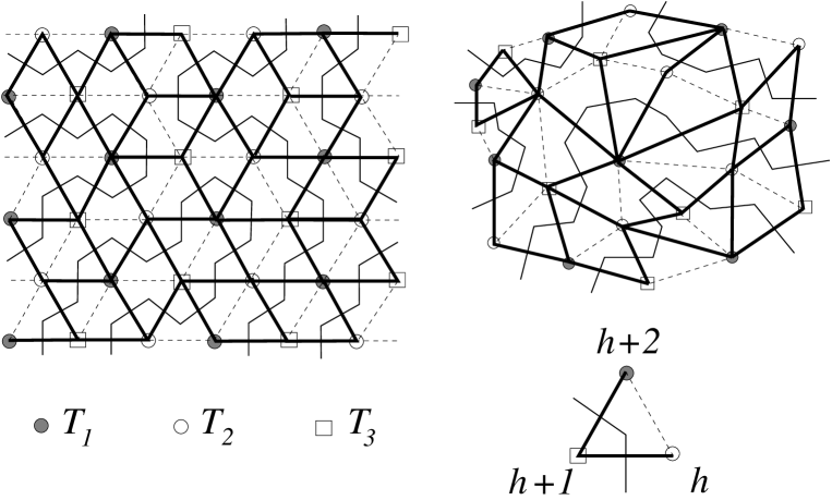
Figure 3: Construction of the SOS degree of freedom from the fully packed loops, on a regular triangular lattice and on a random vertex three-colourable triangulation. The thick lines indicate links whose dual link is occupied by a loop. The height variable $h$, defined on the vertices of the lattice, is such that the difference of height is $\pm 1$ for nearest neighbours connected by a thick line and $\pm 2$ for nearest neighbours connected by a dashed line. The sign is fixed by demanding that $h$ and the number $i$ of the corresponding sub-lattice $T_{i}$ are equal modulo 3. For the regular lattice, this SOS height variable corresponds precisely to the underlying picture of a 2d piling of elementary cubes.

To finish, we may ask how important is the Hamiltonian nature of the walks, or more generally whether or not the fully packing of the (restricted or unrestricted) $O(n)$ model is a relevant constraint. For an $O(n)$ model on the regular honeycomb lattice, it was explained in [8] that the fully packed fixed point differs from the low temperature dense phase fixed point by the emergence of an additional SOS degree of freedom which can be constructed if and only if the loops are fully packed. This degree of freedom is defined as a height variable $h_{v}$ living on the vertices $v$ of the dual triangular lattice (see figure 3). Indeed, this lattice is naturally divided into three alternating sub-lattices $T_{i}$, $i=1,2,3$. Fully packed loops can then be translated into height variables by demanding that $h_{v}=i\ {\rm mod}\ 3$ for $v\in T_{i}$ and by imposing for nearest neighbours $v$ and $v^{\prime}$ that $|h_{v}-h_{v^{\prime}}|=1$ if the link between $v$ and $v^{\prime}$ has its dual link occupied by a loop and $|h_{v}-h_{v^{\prime}}|=2$ if not. This extra SOS degree of freedom results in a shift by 1 of the central charge of the fully packed fixed point with respect to the usual fixed point for the dense phase. On a random lattice, vacancies (i.e. unvisited vertices) can be introduced for instance by adding a term proportional to $A^{3}$ in the potential in (2.1). As shown in [11], on a random lattice the nature of the dense phase fixed point is not changed by eliminating vacancies and the constraint of fully packing is thus irrelevant in this sense. This is also what we find here for $n\rightarrow 0$ where we get $c=-2$ for Hamiltonian walks on a random lattice, as for the dense phase of the $O(n\rightarrow 0)$ model and not $c=-1$ as for the fully packed $O(n\rightarrow 0)$ fixed point describing Hamiltonian walks on the honeycomb lattice. This result is not surprising since, on a random lattice, fully packed loops cannot be transformed anymore into an SOS height variable and we thus expect no shift in the central charge. As a natural question, we may ask whether it is possible to preserve the SOS variable on a random triangular lattice. A SOS variable can be defined in the same way as above if the random lattice can be divided into three alternating sub-lattices. In other words, one needs that the vertices of the lattice can be coloured in three colours such that nearest neighbours have different colours or, stated in yet another way, that any given vertex is shared by an even number of triangles. A vertex three-colouring problem of the above mentioned type was discussed and solved in [18]. Its coupling to a fully packed $O(n)$ model is still an open question but, according to the above discussion we expect the same shift in the central charge as for the regular model. Note that fully packed loops automatically have even length on a vertex three-colourable triangular lattice. The case $n=2$ is of particular interest since it would describe a problem of three-colouring of both the vertices and the edges of random triangulations, a problem equivalent to the folding of random triangulations, as explained in [12, 18]. Based on the discussion above, we expect $c=2$ for this model, as for the fully packed $O(2)$ model on a regular lattice [8].

Acknowledgements     B. Eynard acknowledges the support and the hospitality of the Niels Bohr Institute as well as the support of the European Union through their TMR programme, contract No. ERBFMRXCT 960012. We thank F. David for a critical reading of the manuscript.

References

- [1] M. Gordon, P. Kapadia and A. Malakis, J. Phys. A: Math. Gen. 9 (1976) 751, P.D. Gujrati, J. Phys. A: Math. Gen. 13 (1980) L437, T.G. Schmalz, G. E. Hite and D.J. Klein, J. Phys. A: Math. Gen. 17 (1984) 445, J. Suzuki and T. Izuyama, J. Phys. Soc. Jpn. 57 (1988) 818
- [2] P.W. Kasteleyn, Physica (Utrecht) 29 (1963) 1329
- [3] E.H. Lieb, Phys. Rev. Lett. 18 (1967) 692
- [4] J. Suzuki, J. Phys. Soc. Jpn. 57 (1988) 687
- [5] M.T. Batchelor, J. Suzuki and C.M. Yung, Phys. Rev. Lett. 73 (1994) 2646
- [6] H. Orland, C. Itzykson and C. de Dominics, J. Physique Lett. 46 (1985) L-353
- [7] S. Higuchi, A field theoretic approach to the counting problem of Hamiltonian cycles of graphs, cond-mat/9711152
- [8] H.W.J. Blöte and B. Nienhuis, Phys. Rev. Lett. 72 (1994) 1372
- [9] A. Kast, Correlation length and average loop length of the fully packed loop model, cond-mat/9411132
- [10] I. Kostov, Mod. Phys. Lett. A4 (1989) 217, M. Gaudin and I. Kostov, Phys. Lett. B220 (1989) 200, B. Duplantier and I. Kostov, Phys. Rev. Lett. 61 (1988) 1433 I. Kostov and M. Staudacher, Nucl. Phys. B384 (1992) 459, B. Eynard and J. Zinn-Justin, Nucl. Phys. B386 (1992) 55, B. Eynard and C. Kristjansen, Nucl. Phys. B455 (1995) 577, B. Durhuus and C. Kristjansen, Nucl. Phys. B483 [FS] (1997) 535
- [11] B. Eynard and C. Kristjansen, Nucl. Phys. B466 (1996) 463
- [12] B. Eynard and C. Kristjansen, Nucl. Phys. B516 (1998) 529
- [13] R.J. Baxter, J. Math. Phys. 11 (1970) 784
- [14] G. Cicuta, L. Molinari and E. Montaldi, Phys. Lett. B306 (1993) 245, L. Chekhov and C. Kristjansen, Nucl. Phys. B479 (1996) 683
- [15] E.R. Hansen, A table of series and products, Prentice-Hall 1975
- [16] B. Duplantier and I. Kostov, Nucl. Phys. B340 (1990) 491
- [17] E. Brezin, C. Itzykson, G. Parisi and J.B. Zuber, Comm. Math. Phys. 59 (1978) 35
- [18] P. Di Francesco, B. Eynard and E. Guitter, Nucl. Phys. B516 (1998) 543