[

Energetics of Domain Walls in the 2D $t$-$J$ model

Abstract

Using the density matrix renormalization group, we calculate the energy of a domain wall in the 2D $t$-$J$  model as a function of the linear hole density $\rho_{\ell}$, as well as the interaction energy between walls, for $J/t=0.35$. Based on these results, we conclude that the ground state always has domain walls for dopings $0<x\stackrel{{\scriptstyle<}}{{{}_{\sim}}}0.3$. For $x\stackrel{{\scriptstyle<}}{{{}_{\sim}}}0.125$, the system has (1,0) domain walls with $\rho_{\ell}\sim 0.5$, while for $0.125\stackrel{{\scriptstyle<}}{{{}_{\sim}}}x\stackrel{{\scriptstyle<}}{{{}_{\sim}}}0.17$, the system has a possibly phase-separated mixture of walls with $\rho_{\ell}\sim 0.5$ and $\rho_{\ell}=1$. For $x\stackrel{{\scriptstyle>}}{{{}_{\sim}}}0.17$, there are only walls with $\rho_{\ell}=1$. For $\rho_{\ell}=1$, diagonal (1,1) domain walls have very nearly the same energy as (1,0) domain walls.

]

In the last few years experimental evidence for stripe formation in the cuprates has been mounting[1]. A proper theoretical description of domain walls and striped phases in a doped two-dimensional antiferromagnet has been extremely difficult to develop, however. Although simple mean field theories for the $t$-$J$ or Hubbard models yield domain walls, it is clear that real domain walls have a much more subtly correlated ground state. Partially filled domain walls have been particularly hard to describe theoretically.

Recently, we reported numerical results[2] showing a striped phase in a $16\times 8$ $t$-$J$ system at a filling of $x=0.125$, which were in agreement with neutron scattering results for La_1.6-xNd_0.4Sr_xCuO₄, a system in which a suppression of superconductivity occurs near $x=0.125$. Here, domain walls with a linear filling of 1/2 hole per unit length separating $\pi$-phase-shifted antiferromagnetic regions were spaced four lattice spacings apart. The question of what happens at other fillings was not addressed, and the possibility of other types of domain walls, such as diagonal walls, was not considered. Experimentally, in the Nd_0.4 system Tranquada et. al.[1] report coexistence of superconducting and domain order for a range of dopings away from $x=0.125$. For $0.05\stackrel{{\scriptstyle<}}{{{}_{\sim}}}x\stackrel{{\scriptstyle<}}{{{}_{\sim}}}0.12$, the inverse domain spacing was found to vary as $2x$. Beyond $x=0.12$ the inverse spacing remained relatively constant, increasing slightly as $x$ approached 0.2.

Here we address the question of the stability of domain walls at low to moderate filling, by calculating the energy of a domain wall in the 2D $t$-$J$ model, as a function of filling, using density matrix renormalization group (DMRG)[3] techniques. We use systems with boundary conditions (BCs) carefully chosen not to frustrate the domain walls. We also estimate the repulsive interaction between domain walls, allowing us to study the domain-wall filling and spacing of a striped phase as a function of doping $x$. The DMRG results for energies use extrapolation to extract the limit of zero truncation error[4], with up to 1400 states per block kept. More details of the numerical techniques can be found in [2].

The $t$-$J$  Hamiltonian in the subspace of no doubly occupied sites is given by

$$H=-t\sum_{\langle ij\rangle s}(c_{is}^{\dagger}c_{js}+{\rm h.c.})+J\sum_{\langle ij\rangle}({\bf S}_{i}\!\cdot\!{\bf S}_{j}-\frac{n_{i}n_{j}}{4}).$$ (1)

Here $\langle ij\rangle$ are near-neighbor sites, $s$ is a spin index, ${\vec{S}}_{i}$ and $c^{\dagger}_{i,s}$ are electron spin and creation operators, and $n_{i}=c^{\dagger}_{i\uparrow}c_{i\uparrow}+c^{\dagger}_{i\downarrow}c_{i\downarrow}$. The near-neighbor hopping and exchange interactions are $t$ and $J$. We measure energies in units of $t$. We consider only $J/t=0.35$ here.

First, we consider the energetics of a single domain wall. Imagine a single long domain wall in the form of a closed loop, with a fixed number of holes. The loop would be a large rectangle, if domain walls prefer to be oriented in the (1,0) or (0,1) directions. If we assume that the domain wall is stable against evaporation into holes or pairs, then the loop will adjust its size in order to minimize its energy. The linear hole density $\rho_{\ell}$ of the domain wall will have an optimal value $\bar{\rho}_{\ell}$. We expect that at very low doing, any domain wall will have doping $\bar{\rho}_{\ell}$. At higher doping, repulsion between domain walls could lead to increased values of $\rho_{\ell}$.

Let $e(\rho_{\ell})$ be the energy per hole of a domain wall with density $\rho_{\ell}$. Then $\bar{\rho}_{\ell}$ minimizes $e(\rho_{\ell})$. In order to measure $e(\rho_{\ell})$, some care is needed. The important point is that a loop can shrink or contract without inducing frustration in the antiferromagnetic region inside or out. Therefore, in order to reduce finite size effects, we define $e(\rho_{\ell})$ using two systems, each without frustration. The first system, with energy $E_{\rm dw}$, has a domain wall and BCs favoring the $\pi$-phase shift of the antiferromagnetism induced by the domain wall, while the second, with energy $E_{0}$, has no holes at all and BCs favoring no $\pi$-phase shift, but which are otherwise identical. Defining $N_{\rm dw}$ as the number of holes in the domain wall, we have

$$e(\rho_{\ell})=\frac{E_{\rm dw}-E_{0}}{N_{\rm dw}}$$ (2)

In practice, we use open BCs, with staggered fields on the edges on either side of the domain wall to induce the desired antiferromagnetic order.

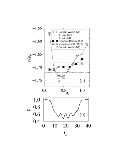
FIG. 1.: (a) Energy per hole of various hole configurations, as discussed in the text. (b) Linear density profile for a $40\times 6$ wall, showing phase separation.

In Fig. 1(a) we show $e(\rho_{\ell})$ as a function of $\rho_{\ell}$, measured on a $16\times 6$ system with open BCs, with the domain wall parallel to the $x$-axis, and with staggered magnetic fields of magnitude $0.1$ applied to the top and bottom rows of sites. We see a minimum at $\bar{\rho}_{\ell}\sim 0.5$. On the same plot, we show by horizontal lines the energy per hole of one hole and of two holes placed in an open $8\times 8$ system, with a staggered field of magnitude $0.1$ on all four sides. The fact that the energy per hole of two holes is lower than that of a single hole indicates that two holes pair-bind, in agreement with exact diagonalization studies[5]. However, the energy of a domain wall at $\bar{\rho}_{\ell}$ is even lower, indicating that domain walls are stable at arbitrarily low doping. To judge the effects of the finite width of the system, results are shown for a $16\times 7$ system at two values of $\rho_{\ell}$. On these larger systems, the energy of the domain wall is lower[6].

The $\rho_{\ell}=1$ domain wall repels additional holes, leading to the rapid increase in $e(\rho_{\ell})$ for $\rho_{\ell}>1$. For $\rho_{\ell}\stackrel{{\scriptstyle<}}{{{}_{\sim}}}0.3$, the holes are too far apart to induce the $\pi$ phase shift of a domain wall. Since our BCs for the doped system require this phase shift, for $\rho_{\ell}\stackrel{{\scriptstyle<}}{{{}_{\sim}}}0.3$ the energy per hole is quite high. In this case BCs without the $\pi$ phase shift give a lower energy, as shown by the stars. However, here we find that the holes bind into isolated pairs rather than a stripe (not shown). The two-hole energy without the $\pi$ phase shift is higher than the two-hole $8\times 8$ line because of larger finite-size effects on the $16\times 6$ system.

The concave nature of the $16\times 6$ domain wall energy for $0.5<\rho_{\ell}<1$ suggests that in this region, a long domain wall will phase separate into a region with $\rho_{\ell}=1$ and a region with $\rho_{\ell}=0.5$. We have directly observed this phase separation in a long $40\times 6$ domain wall. Fig. 1(b) shows the density profile along the wall for $\rho_{\ell}=0.75$. Here the holes have separated into regions with $\rho_{\ell}=1$ and $\rho_{\ell}\sim 0.5-0.6$.

In Fig. 1(a), we also show results for the energy per hole of a diagonal domain wall, using a tilted $12\times 7$ system, which includes seven adjacent (1,1) lines of sites. Similar staggered fields for doped and undoped systems were applied as for the (1,0) walls shown in Fig. 1(a). Here the linear hole density is defined as the number of holes per $\sqrt{2}$ lattice spacings, so that $\rho_{\ell}=1$ corresponds to a filled diagonal wall. The energy near $\rho_{\ell}=1$ is slightly less than the energy of the (1,0) wall; however, the width of the diagonal system is slightly greater. The result shown for a (1,0) domain wall on a $16\times 7$ system shows that the energies are actually nearly degenerate at $\rho_{\ell}=1$. At lower values of $\rho_{\ell}$, (1,0) walls are lower in energy.

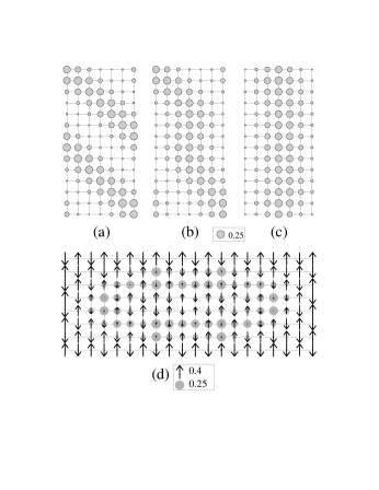
FIG. 2.: (a)-(c) Hole density, showing domain walls in a $14\times 7$ system. The figures are rotated by $90^{\circ}$ for compactness. (d) Hole and spin densities showing a looped wall on a $20\times 8$ system with 16 holes. The diameter of the gray holes and the length of the arrows are proportional to $1-\langle n_{i}\rangle$ and $\langle S^{z}_{i}\rangle$, respectively, according to the scales shown.

In Fig. 2(a)-(c) we show a system which allows either a (1,0) or (1,1) filled domain wall: a $14\times 7$ system with cylindrical BCs (periodic in $y$, open in $x$), doped with 14 holes. Here a single domain wall extends the length of the system. Staggered edge fields on the left and right edges and a small local potential on one site on each edge were used to pin the ends of the domain wall at specified sites. The initial DMRG buildup of the lattice was arranged to initially force an approximate domain wall of the specified form to appear; however, later sweeps allowed the system to relax, although the ends of the walls remained pinned. Within error bars, all three domain wall configurations shown in Fig. 2(a-c) have identical energies. In Fig. 2(a), a (1,1) domain wall wraps around the system. In Fig. 2(b), a wall with both (1,0) and (1,1) parts is present. Notice that the wall resists being situated at an intermediate angle. In Fig. 2(c), a (1,0) domain wall is present. The degeneracy of these states indicates that filled domain walls have the same energy, whether they run in the (1,0) or (1,1) directions. This suggests that filled domain walls might readily fluctuate or form static disordered configurations.

Note that at low doping, in a strictly 2D system, one would expect infinite, straight (1,0) domain walls with filling given by the optimal filling $\bar{\rho}_{\ell}\approx 0.5$. However, in a system with weak coupling to other planes, in order to maintain long range antiferromagnetic order, it is more likely that domain walls would form closed loops, so that most of each plane would be in the dominant antiferromagnetic domain. In Fig. 2(d) we show a loop on a $20\times 8$ system. In this system, staggered fields without any phase shifts were applied to all four sides, preventing a domain wall from ending on a side. Under these circumstances, a loop forms. In a system of weakly coupled planes, the size of a typical loop would be set to balance repulsion between opposite sides of the loop and the exchange cost from the coupling to adjacent planes. (If the exchange coupling between planes were $J^{\prime}\sim 10^{-5}J$, and assuming the repulsion is given by Eq. (3), the loop size would be about 15-20 lattice spacings.) At higher dopings of just a few percent, the interactions between walls would favor the more closely packed striped phases.

In order to understand this interaction between domain walls, we have studied an $L\times 6$ system with cylindrical BCs. In this system, transverse domain walls with four holes wrap around the system, and are stable at low to moderate doping. These walls have $\rho_{\ell}=2/3$. We studied systems with eight or twelve holes, forming two or three domain walls, and studied various lengths $L$ to determine the interaction between the walls. The energy per hole as a function of the domain wall spacing $d$ is shown in Fig. 3(a). The walls repel, rather strongly at short distances. The solid curve in Fig. 3(a) is a simple exponential fit

$$e(d)\equiv e(\infty)+V(d)=e(\infty)+Ae^{-d/w}$$ (3)

with $e(\infty)=-1.79$, $A=0.87$ and $w=1.8$. The source of the repulsion appears to be the finite width of the walls: the hole density distribution spreads out over several lattice spacings. In the insert to Fig. 3(a), we show the hole density per site as a function of $\ell_{x}$ for a $13\times 6$ system with a single domain wall in the center. This gives the density profile of a wall. An isolated wall, far from boundaries in the $L\times 6$ system with $\rho_{\ell}=2/3$, is site-centered. However, walls near boundaries can be more bond-centered; there appears to be little energy difference between walls which are site centered, bond centered, or in between. Notice the substantial width of the wall; only $30\%$ of the hole density is on the center leg. The effective mass of the wall as a whole seems to be very high, so that it is effectively pinned by truncation errors in DMRG. In other words, we believe very little of the apparent width shown is due to uniform motion of the entire wall[7].

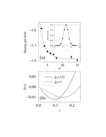
FIG. 3.: (a) Energy per hole of (0,1) domain walls on a $16\times 6$ system, as a function of domain wall separation. The inset shows the transverse hole density in one of the walls. (b) The energy of an array of domain walls as a function of doping $x$.

Using the results of Fig. 1 for the energy per hole in a domain wall and Eq.(3) for the repulsion per hole between domain walls, we consider the relationship between the domain wall spacing $d$ and the doping $x$. The energy per site of an array of domain walls is given by

$$E(\rho_{\ell},d)\equiv x[e(\rho_{\ell})+V(d)].$$ (4)

For $\rho_{\ell}=1/2$, $d=1/(2x)$, while for $\rho_{\ell}=1$, $d=1/x$. For fixed $\rho_{\ell}$, we define

$$E(x)\equiv E(\rho_{\ell},d(x))-x[2e(1)-e(0.5)].$$ (5)

The latter term in Eq. (5) is like a shift in the chemical potential, which allows the curvature in the energy to be seen more easily. In Fig. 3(b), we plot $E(x)$ for $\rho_{\ell}=1/2$ and $\rho_{\ell}=1$ arrays of walls. Clearly, at low values of $x$, all the walls have $\rho_{\ell}=0.5$ and therefore $d^{-1}=2x$. For large values of $x$, all the walls have $\rho_{\ell}=1$ and therefore $d^{-1}=x$. At intermediate values of $x$, $0.11<x<0.16$, using a Maxwell construction one finds a mixture of walls with two different spacings $d_{1/2}$ and $d_{1}$. However, the precise values of $d_{1/2}$ and $d_{1}$ are sensitive to $V(d)$, which was determined only roughly using walls on an $L\times 6$ system with $\rho_{\ell}=2/3$.

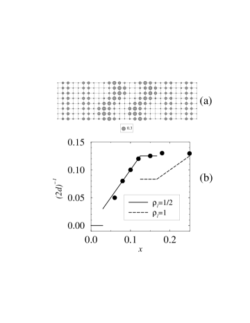
FIG. 4.: (a) Domain walls with $\rho_{\ell}=1$ and $\rho_{\ell}=0.5$ on a $28\times 8$ system, with 32 holes and cylindrical BCs. (b) Shift in the magnetic structure factor peak from $(\pi,\pi)$ as a function of $x$. The solid circles are experimental results[6] for La_2-xSr_xCuO₄.

To determine $d_{1/2}$ and $d_{1}$ more precisely, we have simulated a $28\times 8$ system, with cylindrical BCs, with four (0,1) $\rho_{\ell}=0.5$ walls and two (0,1) $\rho_{\ell}=1.0$ walls, and $x=0.14$. The results are shown in Fig. 4(a). Here, the wall spacings naturally adjust to $d_{1/2}$ and $d_{1}$. We find $d_{1/2}=4$ and $d_{1}=6$, implying that domain wall phase separation occurs for $0.125<x<0.17$. (Note that in this case, the system cannot continuously adjust $\rho_{\ell}$ away from $1/2$ or $1$, and it may be that interactions between walls would shift the $\rho_{\ell}=0.5$ wall to a somewhat different filling.) The resulting inverse domain wall spacing is plotted in Fig. 4(b). Also shown are experimental results[8] for the shift in the magnetic peak in La_2-xSr_xCuO₄. Here we assume that for $x<0.03$ the system has loops rather than stripes so that the magnetic peak would remain at $(\pi,\pi)$. For $x>0.125$, walls with $\rho_{\ell}=1$ and spacing $d_{1}$ give rise to an additional peak, which has not been observed thus far. However, as is obvious from Fig. 4(a), the $\rho_{\ell}=1$ walls seem to be much more subject to disorder and fluctuations, which would significantly weaken and broaden this peak. Observation of this second peak would lend strong support to our results, as would a nonmonotonic shift in the peak near $x\stackrel{{\scriptstyle>}}{{{}_{\sim}}}0.2$.

In our DMRG calculations, large scale fluctuations are difficult to observe, so that a slowly fluctuating striped phase would tend to appear static to us. While this is certainly a disadvantage of DMRG, it makes it easier to rule out uniform phases—phases in which there are no signs of domain walls. In numerous calculations with various BCs, and $x<0.3$, we have not seen a uniform phase[9]. We have observed apparently disordered walls, particularly with $x=0.15-0.20$, but it is difficult to determine in these cases whether an ordered phase is being frustrated by BCs. Note that even if the $\rho_{\ell}=1$ walls are fluctuating or disordered, this probably does not strongly reduce the energy per site relative to the slightly disordered walls shown in Fig. 4(a), so that the phase separation into regions with $\rho_{\ell}=0.5$ walls would be unaffected.

In summary, we find that the (1,0) domain walls formed in the doped $t$-$J$ model have a linear filling $\rho_{\ell}\approx 0.5$ and an inverse spacing $d^{-1}=2x$ for doping $x\stackrel{{\scriptstyle<}}{{{}_{\sim}}}0.125$. For $x\stackrel{{\scriptstyle>}}{{{}_{\sim}}}0.17$, the domain walls have $\rho_{\ell}=1$ and $d^{-1}=x$. It is tempting to identify the underdoped regime with the $\rho_{\ell}=0.5$ walls and the overdoped regime with $\rho_{\ell}=1$. We also find that $\rho_{\ell}=1$ (1,0) walls are nearly degenerate with diagonal (1,1) domain walls, suggesting that these walls may have large fluctuations.

We acknowledge support from the NSF under Grant No. DMR-9509945 (SRW), PHY-9407194 (DJS), and DMR-9527304 (DJS).

REFERENCES

- [1] J.M. Tranquada et al, Nature 375, 561 (1995); Phys. Rev. B54, 7489 (1996); Phys. Rev. Lett.78, 338 (1997).
- [2] S.R. White and D.J. Scalapino, Phys. Rev. Lett.80, 1272 (1998).
- [3] S.R. White, Phys. Rev. Lett.69, 2863 (1992), Phys. Rev. B48, 10345 (1993).
- [4] J. Bonca, J.E. Gubernatis, M. Guerrero, Eric Jeckelmann, and Steven R. White, condmat 9712018.
- [5] E. Dagotto, Rev. Mod. Phys. 66, 763 (1994).
- [6] Given that the finite size corrections are comparable to the differences in energy, we cannot conclusively determine that the domain wall phase is stable at very low doping. However, as can be seen from the curve in Fig. 1(a) labeled “w/o phase shift”, the energy of the pair phase rises rapidly with doping.
- [7] For large , the interaction between walls may become attractive because of a Casimir-like effect. See L. P. Pryadko, S. Kivelson, and D. W. Hone, cond-mat/9711129.
- [8] K. Yamada, C.H. Lee, Y. Endoh, G. Shirane, R.J. Birgeneau, M.A. Kastner, Physica C 282-287, 85 (1997).
- [9] At , we see a quite uniform phase on systems.