Kondo Physics in the Single Electron Transistor with ac Driving

Abstract

Using a time-dependent Anderson Hamiltonian, a quantum dot with an ac voltage applied to a nearby gate is investigated. A rich dependence of the linear response conductance on the external frequency and driving amplitude is demonstrated. At low frequencies the ac potential produces sidebands of the Kondo peak in the spectral density of the dot, resulting in a logarithmic decrease in conductance over several decades of frequency. At intermediate frequencies, the conductance of the dot displays an oscillatory behavior due to the appearance of Kondo resonances of the satellites of the dot level. At high frequencies, the conductance of the dot can vary rapidly due to the interplay between photon-assisted tunneling and the Kondo resonance.

It has been predicted that, at low temperatures, transport through a quantum dot should be governed by the same many-body phenomenon that enhances the resistivity of a metal containing magnetic impurities – namely the Kondo effect [1]. The recent observation of the Kondo effect by Goldhaber et al.[2] in a quantum dot operating as a single-electron transistor (SET) has fully verified these predictions. In contrast to bulk metals, where the Kondo effect corresponds to the screening of the free spins of a large number of magnetic impurities, there is only one free spin in the quantum-dot experiment. Moreover, a combination of bias and gate voltages allow the Kondo regime, mixed-valence regime, and empty-site regime all to be studied for the same quantum dot, both in and out of equilibrium[2].

Here we consider another opportunity presented by the observation of the Kondo effect in a quantum dot that is not available in bulk metals – the application of an unscreened ac potential. There is already a large literature concerning the experimental application of time-dependent fields to quantum dots [3]. For a dot acting as a Kondo system, the ac voltage can be used to periodically modify the Kondo temperature or to alternate between the Kondo and mixed-valence regimes. Thus it is natural to ask what additional phenomena occur in a driven system which in steady state is dominated by the Kondo effect [4, 5]. Our results indicate a rich range of behavior with increasing ac frequency, from sidebands of the Kondo peak at low ac frequencies, to conductance oscillations at intermediate frequencies, and finally to photon-assisted tunneling at high ac frequencies.

The system of interest is a semiconductor quantum dot, as pictured schematically in Fig. 1. An electron can be constrained between two reservoirs by tunneling barriers leading to a virtual electronic level within the dot at energy $\sim$$\epsilon_{\rm dot}$ (measured from the Fermi level) and width $\sim$$2\Gamma_{\rm dot}$ [6]. We assume that both the charging energy $e^{2}/C$ and the level spacing in the dot are much larger than $\Gamma_{\rm dot}$, so the dot will operate as a SET [3]. In this work, we consider only the linear-response conductance between the two reservoirs. However, we will allow an oscillating gate voltage $V_{\rm g}(t)=V_{0}+V_{\rm ac}\cos\Omega t$ of arbitrary (angular) frequency $\Omega$ and arbitrary amplitude $V_{\rm ac}$, which modulates the virtual-level energy $\epsilon_{\rm dot}(t)$.

Such a system may be described by a constrained ($U=\infty$) Anderson Hamiltonian

$$\sum_{\sigma}\!\epsilon_{\rm dot}(t)\,n_{\sigma}+\sum_{k\sigma}\!\left[\epsilon_{k\sigma}n_{k\sigma}+(V_{k}c^{\dagger}_{k\sigma}c_{\sigma}+{\rm H.c.})\right].$$ (1)

Here $c^{\dagger}_{\sigma}$ creates an electron of spin $\sigma$ in the quantum dot, while $n_{\sigma}$ is the corresponding number operator; $c^{\dagger}_{k\sigma}$ creates a corresponding reservoir electron; $k$ is shorthand for all other quantum numbers of the reservoir electrons, including the designation of left or right reservoir, while $V_{k}$ is the tunneling matrix element through the appropriate barrier. Because the charging energy to add a second electron, $U=e^{2}/C$, is assumed large, the Fock space in which the Hamiltonian (1) operates is restricted to those elements with zero or one electron in the dot.

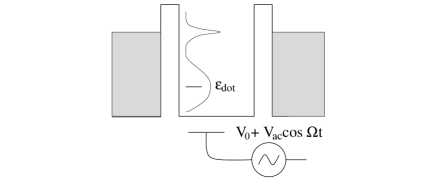
FIG. 1.: Schematic picture of the quantum dot SET.

At low temperatures, the Anderson Hamiltonian (1) gives rise to the Kondo effect when the level energy $\epsilon_{\rm dot}$ lies below the Fermi energy. In this regime, a single electron occupies the dot which, in effect, turns the dot into a magnetic impurity with a free spin. The temperature required to observe the Kondo effect in linear response is of order $T_{\rm K}\sim D\exp(-\pi|\epsilon_{\rm dot}|/\Gamma_{\rm dot})$, where $D$ is the energy difference between the Fermi level and the bottom of the band of states. For the temperature range that is likely to be experimentally accessible in a SET, $T\sim T_{\rm K}$ or higher, there exists a well tested and reliable approximation known as the non-crossing approximation (NCA) [7]. The NCA has been formally generalized to the full time-dependent nonequilibrium case [8], and an exact method for the (numerical) solution implemented [9]. The time-dependent NCA has been applied to Kondo physics in charge transfer in hyperthermal ion scattering from metallic surfaces [9, 10] and to energy transfer and stimulated desorption at metallic surfaces [11]. An independent formulation [4] has been applied to quantum dots, although the high frequency expansion used there appears limited. Here we present the exact time-dependent NCA solution for a quantum dot over the full range of applied frequencies.

The time-dependent electronic structure of the dot can be characterized by the time-dependent spectral density

$$\rho_{\rm dot}(\epsilon,t)\equiv\int_{-\infty}^{\infty}\frac{d\tau}{2\pi}e^{i\epsilon\tau/\hbar}\langle\{c_{\sigma}(t+\frac{1}{2}\tau),c_{\sigma}^{\dagger}(t-\frac{1}{2}\tau)\}\rangle$$ (2)

evaluated in the restricted Fock space. For the equilibrium Kondo system, $\rho_{\rm dot}(\epsilon)$ is time independent, and looks like the graph in the schematic in Fig. 1. Roughly speaking, $\rho_{\rm dot}(\epsilon)$ consists of a broad peak of width $\sim$$2\Gamma_{\rm dot}$ at the level position $\epsilon_{\rm dot}$ and a sharp Kondo peak of width $\sim$$T_{\rm K}$ near the Fermi level. We will refer to these features as the virtual-level peak and the Kondo peak, respectively. In the steady-state case, the linear-response conductance $G$ through a dot symmetrically coupled to two reservoirs is given by [12]

$$G={e^{2}\over\hbar}{{\Gamma_{\rm dot}}\over{2}}\int\!d\epsilon\,\rho_{\rm dot}(\epsilon)\left(-\frac{\partial f(\epsilon)}{\partial\epsilon}\right),$$ (3)

where $f(\epsilon)$ is the Fermi function. The formula (3) will still be valid in the case where the gate voltage is time dependent if $G$ is the time-averaged conductance and $\rho_{\rm dot}(\epsilon)$ is replaced by the time-averaged spectral density $\langle\rho_{\rm dot}(\epsilon,t)\rangle$ [13, 14]. For a given system, this average will depend on the driving amplitude $V_{\rm ac}$ and frequency $\Omega$.

FIG. 2.: The spectral density $\langle\rho_{\rm dot}(\epsilon,t)\rangle$ vs. energy $\epsilon$ for a quantum dot with level energy $\epsilon_{\rm dot}(t)=-5+4\cos\Omega t$ and $T=0.005$. The non-driven case is also shown in the final panel. Throughout this letter, energies are in units of $\Gamma_{\rm dot}$.

In Fig. 2 we show the calculated $\langle\rho_{\rm dot}(\epsilon,t)\rangle$ as a function of energy $\epsilon$ for a level with energy $\epsilon_{\rm dot}(t)=\epsilon_{\rm dot}+\epsilon_{\rm ac}\cos\Omega t$ at several different frequencies $\Omega$. The corresponding conductance is shown by the curve labeled dot A, $T=0.005$ in Fig. 3. For the lowest $\Omega$, the response of the system is relatively adiabatic and the displayed spectral function resembles the spectral function that would have resulted if the system had been in perfect equilibrium for all the dot level positions over a period of oscillation of $\epsilon_{\rm dot}(t)$. The two broad peaks are the influence of the virtual level peaks at the two stationary points of this oscillation (here at $\epsilon=-1$ and $\epsilon=-9$). As the frequency $\Omega$ is increased, marked nonadiabatic effects result, the most obvious being the appearance of multiple satellites around the Kondo resonance [4]. These sidebands appear at energies equal to $\hbar$ times multiples of the driving frequency $\Omega$ [15]. As the frequency $\Omega$ is increased, spectral weight is transferred from the main Kondo peak to these satellites. As the conductance is dominated by $\langle\rho_{\rm dot}(\epsilon,t)\rangle$ at the Fermi energy, this causes the slow logarithmic falloff of the conductance over two decades of frequency, as shown in Fig. 3.

As $\hbar\Omega$ becomes larger than $\Gamma_{\rm dot}$, inspection of Fig. 2 shows that broad satellites also appear at energy separations $n\hbar\Omega$ around the average virtual-level position $\epsilon_{\rm dot}$. These satellites of the virtual level are the analogues of those predicted in the noninteracting case [13], which decrease in magnitude as the order $n$ of the Bessel function $J_{n}$. Here, however, the virtual-level satellites have their own Kondo peaks; each of the latter gets strong when the corresponding virtual-level satellite reaches a position a little below the Fermi level, and then disappears as the broad satellite crosses the Fermi level. This effect produces the oscillations in the conductance that are evident in the lower curves in Fig. 3. These oscillations are very different from those that would occur in a noninteracting ($U=0$) case: due to the Kondo peaks they are substantially stronger, their maxima occur at different frequencies and their magnitudes are temperature dependent. As the last virtual-level satellite crosses the Fermi level, $\hbar\Omega=|\epsilon_{\rm dot}|$, the dot level energy begins to vary too fast for the system to respond and the average spectral function approaches (exactly as $\Omega\rightarrow\infty$) the equilibrium spectral function for a dot level centered at the average position $\epsilon_{\rm dot}$. For the parameters of Fig. 2, the high frequency region is uninteresting, because the temperature is far above the Kondo temperature. Therefore, the conductance shows little temperature or frequency dependence at these high frequencies.

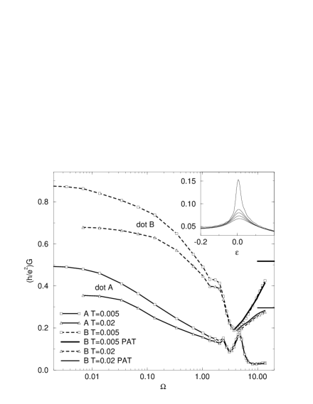
FIG. 3.: Conductance of two different quantum dots, each at two different temperatures: Dot A, $\epsilon_{\rm dot}(t)=-5+4\cos\Omega t$; Dot B, $\epsilon_{\rm dot}(t)=-2.5+2\cos\Omega t$. The curves at the high $\Omega$ end for dot B (marked “PAT”) are from our photon-assisted-tunneling model, while the exact high frequency asymptotes for dot B are shown as short horizontal lines extending from the right vertical axis. The inset shows the spectral density $\langle\rho_{\rm dot}(\epsilon,t)\rangle$ of dot B around the Fermi level, at $T=0.005$, for large frequencies, from $\Omega=4.8$ (lowest curve), through 5.5, 6.1, 6.8 to $\Omega=14$ (topmost curve).

The situation is quite different for the system (dot B) displayed in the upper two curves in Fig. 3, which displays a strong Kondo effect when the dot level is held at its average energy $\epsilon_{\rm dot}$. In this case the $\Omega\rightarrow\infty$ conductance is strongly enhanced by the Kondo effect, and is consequently temperature dependent as well. Note that the conductance falls off significantly from its asymptotic, $\Omega\rightarrow\infty$, value for frequencies still much larger than either the depth of the level $|\epsilon_{\rm dot}|$ or its width. This effect is due to a rapid decline of the amplitude of the Kondo peak in the spectral density, as illustrated in the inset of Fig. 3. We propose the following explanation for this phenomenon. The energy $\hbar\Omega$ excites the dot, producing satellites [16, 13] of the virtual level peak at energies $\epsilon_{\rm dot}\pm n\hbar\Omega$, which, for $\hbar\Omega\gg\Gamma_{\rm dot}$ have strength roughly given by $[J_{n}(\epsilon_{\rm ac}/\hbar\Omega)]^{2}$ as in the $U=0$ case (see Fig. 2 and the previous discussion). For large $\hbar\Omega$, only the two $n=1$ satellites have any significant strength, and the higher lies above the Fermi level, allowing an electron on the dot to decay at the rate $(1/\hbar)\Gamma_{\rm dot}(\epsilon_{\rm dot}+\hbar\Omega)$. The overall electron decay probability per unit time $\Gamma_{\rm decay}/\hbar$ due to this photon-assisted-tunneling mechanism (PAT) is therefore given by

$$\Gamma_{\rm decay}\approx[J_{1}(\epsilon_{\rm ac}/\hbar\Omega)]^{2}\,\Gamma_{\rm dot}(\epsilon_{\rm dot}+\hbar\Omega).$$ (4)

The above rate carries with it an energy uncertainty, which we speculate has roughly the same effect on the Kondo peak as the energy smearing due to a finite temperature. We can test this conjecture by calculating the equilibrium conductance at an effective temperature $T_{\rm eff}$ given by $T_{\rm eff}=T+\Gamma_{\rm decay}$. The results of such a calculation are shown in Fig. 3 (PAT curves), where they compare very favorably with our results for the conductance in the ac-driven system.

Returning to the behavior at low frequencies, we find that it can be best understood in terms of the Kondo Hamiltonian, which, with respect to properties near the Fermi level, is equivalent to the Anderson Hamiltonian (1) in the extreme Kondo region $-\epsilon_{\rm dot}\gg\Gamma_{\rm dot}$ [17]. In this limit the dot can be replaced simply by a dynamical Heisenberg spin $\vec{S}$ ($S^{2}=\frac{3}{4}$), which scatters electrons both within and between reservoirs. The Kondo Hamiltonian corresponding to the Anderson model (1) is

$$\sum_{kk^{\prime}\sigma\sigma^{\prime}}J_{kk^{\prime}}(t)\left(\vec{S}\cdot\vec{\sigma}_{\sigma\sigma^{\prime}}+\frac{1}{2}\delta_{\sigma\sigma^{\prime}}\right)c^{\dagger}_{k\sigma}c_{k^{\prime}\sigma^{\prime}},$$ (5)

where the components of $\vec{\sigma}$ are the Pauli spin matrices. For near Fermi level properties we can suppress the detailed $k$ dependence of $J$ and $V$ and introduce a large energy cutoff $D$ [18], in which case the relationship between the Kondo and Anderson Hamiltonians [17] is $J(t)=|V^{2}/\epsilon_{\rm dot}(t)|$ for our $U=\infty$ case. If we let $w_{\rm leads}(\epsilon)/\hbar$ be the total rate at which lead electrons of energy $\epsilon$ undergo intralead and interlead scattering by the dot, then $w_{\rm leads}(\epsilon)$ will have a Kondo peak for $\epsilon$ near the Fermi level. Furthermore, if $J$ is modulated as $J(t)={\langle{J}\rangle}(1+\alpha\cos\Omega t)$, then an electron scattered by the dot will be able to absorb or emit multiple quanta of energy $\hbar\Omega$, leading to satellites of the Kondo peak in $\langle\rho_{\rm dot}(\epsilon,t)\rangle$ through the exact Anderson model relation

FIG. 4.: Spectral density $\langle\rho_{\rm dot}(\epsilon,t)\rangle$ times $10^{3}$ in the Kondo model and NCA for $T=0.02$ and ${\langle{J}\rangle}\rho=0.023$ ($\epsilon_{\rm dot}=-7$). For the non-driven case (left panel) we also show the comparable result from summing all the leading logarithmic terms (Abrikosov, Ref. [19]), as well as that obtained to order $J^{2}$. The energy dependence of ${\langle{J}\rangle}$ (Ref. [17]) has been included to order $J^{2}$ in all the Kondo Hamiltonian curves.

$w_{\rm leads}(\epsilon)$. This then reflects back on

$$w_{\rm leads}(\epsilon)=\Gamma_{\rm dot}(\epsilon)\langle\rho_{\rm dot}(\epsilon,t)\rangle/\rho_{\rm leads}(\epsilon),$$ (6)

where $\rho_{\rm leads}(\epsilon)$ is the state density per spin in the leads.

The above can be illustrated explicitly using perturbation theory in $J$. Keeping all terms of order $J^{2}$ and logarithmic terms to order $J^{3}$, we find, using a nonequilibrium version of Abrikosov’s pseudofermion technique [19], that

$$w_{\rm leads}(\epsilon)=2\pi\langle J^{2}\rangle\rho\bigg{[}1+3\langle{J}\rangle\rho\sum_{n=-1}^{1}a_{n}g(\epsilon+n\hbar\Omega)\bigg{]},$$ (7)

where $\rho=\rho_{\rm leads}(0)$, $a_{0}=1$, $a_{\pm 1}=\alpha^{2}/(2+\alpha^{2})$, $\langle J^{2}\rangle=(1+\frac{1}{2}\alpha^{2}){\langle{J}\rangle}^{2}$, and

$$g(\epsilon)=\frac{1}{2}\int_{-D}^{D}\!d\epsilon^{\prime}\,\frac{1-2f(\epsilon^{\prime})}{\epsilon^{\prime}-\epsilon}\rightarrow\ln\left|\frac{D}{\epsilon}\right|,$$ (8)

the last limit being approached when $T\ll|\epsilon|$. In Fig. 4 we compare this prediction with the full NCA theory. Although we are not strictly in the parameter region where the $J^{3}$ theory is quantitatively valid, the qualitative agreement is quite satisfactory.

The present results indicate rich behavior when an external ac potential is applied to a quantum dot in the regime where the conductance is dominated by the Kondo effect. While the time-dependent NCA method employed spans the full range of applied frequency, some additional insight has been gained into the behavior both at very low and very high frequencies. At low frequencies a time-dependent Kondo model helps explain the amplitudes of sidebands of the Kondo peak in the spectral density of the dot. At high frequencies, a cutoff of the Kondo peak due to photon-assisted tunneling processes accounts for the reduction of conductance. We hope that our work will inspire experimental investigation of these phenomena and other ramifications of ac driving applied to Kondo systems.

The work was supported in part by NSF grants DMR 95-21444 (Rice) and DMR 97-08499 (Rutgers), and by US-Israeli Binational Science Foundation grant 94-00277/1 (BGU).

REFERENCES

- [1] L. I. Glazman and M. E. Raikh, Pis’ma Zh. Eksp. Teor. Fiz. 47, 378 (1988) [JETP Lett. 47, 452 (1988)]; T. K. Ng and P. A. Lee, Phys. Rev. Lett. 61, 1768 (1988); S. Hershfield, J. H. Davies, and J. W. Wilkins, Phys. Rev. Lett. 67, 3720 (1991); Y. Meir, N. S. Wingreen, and P. A. Lee, Phys. Rev. Lett. 70, 2601 (1993); N. S. Wingreen and Y. Meir, Phys. Rev. B 49, 11 040 (1994).
- [2] D. Goldhaber-Gordon et al., Nature 391, 156 (1998).
- [3] L. P. Kouwenhoven et al., in Mesoscopic Electron Transport, edited by L. L. Sohn, L. P. Kouwenhoven, and G. Schön (Kluwer, Netherlands, 1997).
- [4] M. H. Hettler and H. Schoeller, Phys. Rev. Lett. 74, 4907 (1995).
- [5] A. Schiller and S. Hershfield, Phys. Rev. Lett. 77, 1821 (1996); T. K. Ng, Phys. Rev. Lett. 76, 487 (1996); Y. Goldin and Y. Avishai, preprint cond-mat/9710085.
- [6] We define , a slowly varying quantity. The notation with no energy specified will always refer the value at the Fermi level.
- [7] N. E. Bickers, Rev. Mod. Phys. 59, 845 (1987).
- [8] D. C. Langreth and P. Nordlander, Phys. Rev. B 43, 2541 (1991).
- [9] H. Shao, D. C. Langreth, and P. Nordlander, Phys. Rev. B 49, 13 929 (1994).
- [10] H. Shao, P. Nordlander, and D. C. Langreth, Phys. Rev. B 52, 2988 (1995), Phys. Rev. Lett. 77, 948 (1996).
- [11] T. Brunner and D. C. Langreth, Phys. Rev. B 55, 2578 (1997); M. Plihal and D. C. Langreth, Surf. Sci. Lett. 395, 252 (1998); Phys. Rev. B (submitted).
- [12] Y. Meir and N. S. Wingreen, Phys. Rev. Lett. 68, 2512 (1992).
- [13] A.-P. Jauho, N. S. Wingreen, and Y. Meir, Phys. Rev. B 50, 5528 (1994).
- [14] For the Hamiltonian (1) the time average , where is the retarded and hence causal function defined in Ref. [13], Eq. (28).
- [15] Hence in an experiment one may also expect peaks spaced by in the differential conductance.
- [16] P. K. Tien and J. P. Gordon, Phys. Rev. 129, 647 (1963).
- [17] J. R. Schrieffer and P. A. Wolff, Phys. Rev. 149, 491 (1966).
- [18] For the lead state density used in the NCA calculations, , the appropriate value is given by ; see Ref. [9].
- [19] A. A. Abrikosov, Physics 2, 5 (1965).