Cotunneling and renormalization effects for the single-electron transistor

Abstract

We study electron transport through a small metallic island in the perturbative regime. Using a diagrammatic real-time technique, we calculate the occupation of the island as well as the conductance through the transistor at arbitrary temperature and bias voltage in forth order in the tunneling matrix elements, a process referred to as cotunneling. Our formulation does not require the introduction of a cutoff. At resonance we find significant modifications of previous theories and quantitative agreement with recent experiments. We determine the renormalization of the system parameters and extract the arguments of the leading logarithmic terms (which can not be derived from usual renormalization group analysis). Furthermore, we perform the low- and high-temperature limits. In the former, we find a behavior characteristic for the multichannel Kondo model.

I Introduction

Electron transport through small metallic islands is strongly influenced by the charging energy associated with low capacitance of the junctions [1, 2, 3]. A variety of single-electron effects, including Coulomb blockade phenomena and gate-voltage dependent oscillations of the conductance, have been observed. If the conductance of the barriers is low

$$\alpha_{0}\equiv h/(4\pi^{2}e^{2}R_{\rm T})\ll 1$$ (1)

they can be described within the “orthodox theory”[1] which treats tunneling in lowest order perturbation theory (golden rule). This corresponds to the classical picture of incoherent, sequential tunneling processes. On the other hand, there is experimental and theoretical evidence that in several regimes higher-order tunneling processes have to be taken into account.

First, in the Coulomb blockade regime, sequential tunneling is exponentially suppressed. The leading contribution to the current is a second-order process in $\alpha_{0}$ where electrons tunnel via a virtual state of the island. In Ref. [4] the transition rate of this “inelastic cotunneling” process was evaluated at zero temperature. A divergence arises at finite temperature which requires a regularization. In Ref. [4] this was done within an approximation which is valid far away from the resonances. In this regime, their results have been confirmed by experiments [5].

Second, at resonance, even though sequential tunneling occurs, higher-order processes have a significant effect on the gate-voltage dependent linear and nonlinear conductance [6, 7, 8]. The energy gap between two adjacent charge states as well as the tunneling conductance is renormalized. Similar effects have been discussed for the equilibrium properties of the single-electron box [9, 10, 11, 12, 13]. A diagrammatic real-time technique developed for metallic islands [6, 7] as well as for quantum dots [14, 15] allows a systematic description of the nonequilibrium tunneling processes. The effects of quantum fluctuations become observable either for strong tunneling $\alpha_{0}\sim 1$ or at low temperatures $\alpha_{0}\ln({E_{\rm C}/T})\sim 1$, where $E_{\rm C}$ denotes the charging energy (see below). The theory has been evaluated in Ref. [6, 7] in the limit where only two adjacent charge states are included (even virtually). Therefore, it was necessary to introduce a bandwidth cutoff $\sim E_{\rm C}$. The predicted broadening of the conductance peak as well as the reduction of its height has been confirmed qualitatively in recent experiments on a single-electron transistor in the strong tunneling regime by Joyez et al. [16]. However, a quantitative fit between theory and experiment requires introducing a renormalized value for the charging energy.

In Ref. [8], we have used the real-time diagrammatic technique to obtain the current in second order in $\alpha_{0}$ at low temperature when only two adjacent charge states are classically occupied, but all relevant virtual states are included. In this case no cutoff is required; all terms are regularized in a natural way. This analysis allows an unambiguous comparison with experiments where only bare system parameters enter. At resonance we obtain new contributions compared to the earlier theory of electron cotunneling. They emerge from a renormalization of the charge excitation energy and the tunneling conductance. For realistic parameters $T/E_{\rm C}\sim 0.05$ and $\alpha_{0}^{\rm L}=\alpha_{0}^{\rm R}\sim 0.02$ the corrections are of order $20\%$.

In this article, we generalize the analysis of Ref. [8] in the following points:
– We allow for arbitrary temperature. Our theory is, therefore, applicable both in the Coulomb blockade regime at low temperature as well as the classical regime at high temperature. While the effects of cotunneling are most dramatic in the first case, signatures of the higher order contributions are visible even in the second case.
– We allow for arbitrary transport voltage, i.e., also extreme non-equilibrium situations are included in which more than two charge states are classically occupied.
– We present analytic expressions for the current, and we discuss the asymptotic behavior at low and high temperatures. Renormalization group studies of the single-electron box [10, 12] predict a renormalization of the system parameters, which depends logarithmically on the relevant energy scale. This renormalization shows up in our formulas in new terms which are crucial at resonance. We are, therefore, able to extract the argument of the leading logarithmic terms. Finally, we compare with recent experiments [16] and find very good agreement without any fitting parameter.

This paper is organized as follows:

In Sec. II we define the model, which is based on the standard tunneling Hamiltonian, and describe the diagrammatic technique which we use in the following. We, then, set up the general scheme for a systematic perturbation expansion in the dimensionless conductance $\alpha_{0}$ in Sec. III.

Sec. IV contains the general result for the expansion up to second order, in which we find four terms contributing to the total current $I^{(2)}=I^{(2)}_{1}+I^{(2)}_{2}+I^{(2)}_{3}+I^{(2)}_{4}$, Eqs. (28)-(36). The first one, $I^{(2)}_{1}$, is related to processes in which one electron enters and another one leaves the island coherently. This term is responsible for a finite transport in the Coulomb blockade regime. We recover the usual ”cotunneling” [4] but without any regularization problems at finite temperature. The second and third contribution, $I^{(2)}_{2}$ and $I^{(2)}_{3}$, describe the renormalization of the dimensionless conductance and of the energy gap for adjacent charge states, respectively. These terms are important at resonance. The fourth contribution, $I^{(2)}_{4}$, corresponds to processes in which two electrons enter or leave the island coherently. This plays a role in situations in which more than two charge states are classically occupied, i.e., at high temperature or high voltage. For a quantitative comparison with experiments [16] all terms are important.

The results simplify to closed analytic expressions in the two most interesting cases. The first is the low temperature regime (Sec. V) in which the renormalization of the system parameters plays an important role. The dimensionless conductance as well as the energy gap between adjacent charge states are effectively reduced. A discussion of this renormalization and a comparison is given in Sec. VI.

The other case in which we obtain closed analytic expressions is the linear response regime for arbitrary temperature (Sec. VII). We finally perform an expansion for low and high temperatures, respectively, and obtain very simple results for these limits in Sec. VIII.

In general a numerical solution of a set of equations is necessary to evaluate the contribution $I^{(2)}_{2}$.

II The Model and diagrammatic technique

The single-electron transistor (see Fig. 1) is modeled by the Hamiltonian

$$H=H_{\rm L}+H_{\rm R}+H_{\rm I}+H_{\rm ch}+H_{\rm T}=H_{0}+H_{\rm T}.$$ (2)

Here $H_{\rm r}=\sum_{kn}\epsilon^{\rm r}_{kn}a^{\dagger}_{{\rm r}kn}a_{{\rm r}kn}$ and $H_{\rm I}=\sum_{qn}\epsilon_{qn}c^{\dagger}_{qn}c_{qn}$ describe the noninteracting electrons in the two leads r=L,R and on the island. The index $n=1,\dots N$ is the transverse channel index which includes the spin while the wave vectors $k$ and $q$ numerate the states of the electrons within one channel. In the following, we consider “wide” metallic junctions with $N\gg 1$. The Coulomb interaction of the electrons on the island is described by the capacitance model $H_{\rm ch}=E_{\rm C}(\hat{n}-n_{\rm x})^{2}$, where $E_{\rm C}=e^{2}/(2C)$ with $C=C_{\rm L}+C_{\rm R}+C_{\rm g}$. The excess particle number operator on the island is given by $\hat{n}$. Furthermore, the ’external charge’ $en_{\rm x}=C_{\rm L}V_{\rm L}+C_{\rm R}V_{\rm R}+C_{\rm g}V_{\rm g}$, accounts for the applied gate and transport voltages. The charge transfer processes are described by the tunneling Hamiltonian

$$H_{\rm T}=\sum_{\rm r=L,R}\sum_{kqn}T^{{\rm r}n}_{kq}a^{\dagger}_{{\rm r}kn}c_{qn}{\rm e}^{-i\hat{\varphi}}+{\rm h.c.}\;.$$ (3)

The matrix elements $T^{{\rm r}n}_{kq}$ are considered independent of the states $k$ and $q$ and the channel $n$. They are related to the tunneling resistances $R_{\rm T,r}$ of the left and right junction by $1/R_{\rm T,r}=(2\pi e^{2}/\hbar)NN_{\rm r}(0)N_{I}(0)|T^{{\rm r}n}|^{2}$, where $N_{\rm I/r}(0)$ are the density of states of the island/leads at the Fermi level. The operator ${\rm e}^{\pm i\hat{\varphi}}$ keeps track of the change of the charge on the island by $\pm e$.

We proceed using the diagrammatic technique developed in Refs. [6, 7]. The nonequilibrium time evolution of the charge degrees of freedom on the island is described by a density matrix, which we expand in $H_{\rm T}$. The reservoirs are assumed to remain in thermal equilibrium (with electrochemical potential $\mu_{\rm r}$) and are traced out using Wick’s theorem, such that the Fermion operators are contracted in pairs. For a large number of channels $N$, the “simple loop” configurations dominate where the two operators in $a^{\dagger}_{{\rm r}kn}c_{qn}$ from one term $H_{\rm T}$ are contracted with the corresponding two operators $c^{\dagger}_{qn}a_{{\rm r}kn}$ from another term $H_{\rm T}$, while the contribution of more complicated configurations are small.

The time evolution of the reduced density matrix in a basis of charge states is visualized in Fig. (2). The forward and backward propagator (on the Keldysh contour) are coupled by “tunneling lines”, representing tunneling in junction ${\rm r}$. In Fourier space they are given by

$$\alpha^{\pm}_{\rm r}(\omega)=\pm\alpha_{0}^{\rm r}{\omega-\mu_{\rm r}\over\exp[\pm\beta(\omega-\mu_{\rm r})]-1}\,.$$ (4)

if the line is directed backward/forward with respect to the closed time path. Furthermore, we associate with each tunneling vertex at time $t$ a factor $\exp{(\pm i\Delta_{n}\,t)}$ depending on the energy difference of the adjacent charge states

$$\Delta_{n}=E_{\rm ch}(n+1)-E_{\rm ch}(n)=E_{C}\left[1+2(n-n_{x})\right].$$ (5)

If the vertex lies on the backward path it acquires a factor $-1$. We define $\alpha_{0}=\sum_{\rm r}\alpha_{0}^{\rm r}$ and $\alpha(\omega)=\sum_{\rm r}\alpha_{\rm r}(\omega)$.

The time evolution of the system is determined by an infinite sequence of transitions between different charge states (see Fig. 2). This leads to a stationary probability distribution $p_{n}$ at the end. As shown in Refs. [6, 7] the probabilities $p_{n}$ are described by a master equation which reads in the stationary limit

$$0=\sum\limits_{n^{\prime}\neq n}\left[p_{n^{\prime}}\Sigma_{n^{\prime},n}-p_{n}\Sigma_{n,n^{\prime}}\right]\,.$$ (6)

Here $\Sigma_{n,n^{\prime}}$ denotes the transition rate between $n$ and $n^{\prime}$. Only the latest transition, i.e., the rightmost irreducible part in the diagrams, is written explicitly. (We call a diagram part irreducible if there is no possible vertical cut separating the diagram into two parts.) The sequence of the preceding transitions is summarized in the stationary probability $p_{n}$ of charge state $n$.

The tunneling current $I_{\rm r}$ flowing into reservoir r can be expressed in terms of the correlation functions for the island charge

$$C^{>}(t,t^{\prime}) = -i\langle e^{-i\varphi(t)}e^{i\varphi(t^{\prime})}\rangle\,,$$ (7)

$$C^{<}(t,t^{\prime}) = i\langle e^{i\varphi(t^{\prime})}e^{-i\varphi(t)}\rangle\,.$$ (8)

Since the system is time-translational invariant, the correlation functions depend only on the time difference $C(t,t^{\prime})=C(t-t^{\prime})$, and we can define the Fourier transforms $C(\omega)=\int dte^{i\omega t}C(t)$. As shown in Refs. [6, 7] the tunneling current is

$$I_{\rm r}=-ie\int d\omega\left\{\alpha_{\rm r}^{+}(\omega)C^{>}(\omega)+\alpha_{\rm r}^{-}(\omega)C^{<}(\omega)\right\}\,.$$ (9)

For each contribution to the correlation functions the corresponding diagram contains two external vertices (representing the $e^{\pm i\varphi}$ terms in Eqs. (7) and (8) ) connected by a solid line. Two examples are shown in Fig. 3. The value of the diagram is given by the probability of the states indicated on the left hand side of the diagram ($p_{n}$ in Fig. 3) multiplied with the value of the irreducible diagram part (consisting of two lines in Fig. 3). The probability includes the sequence of preceding transitions which are disconnected from the latest irreducible part. While the calculation of the irreducible part follows straightforward from the diagram rules, we need some extra relation in order to determine the stationary probabilities $p_{n}$. This relation can be the master equation Eq. (6). But instead of Eq. (6) we use an alternative condition which is equivalent to the master equation.

For this task we introduce the quantities $C(\omega,n)$, $I_{\rm r}(n)$ and $I(n)=\sum_{\rm r}I_{\rm r}(n)$ as the contribution to the correlation function and current in which the rightmost vertex describes a transition from $n$ to $n+1$ or vice versa. We can prove current conservation not only for the total current $\sum_{\rm r}I_{\rm r}=0$ but also for each part $I(n)=0$ [17], i.e.,

$$\int d\omega\left\{\alpha^{+}(\omega)C^{>}(\omega,n)+\alpha^{-}(\omega)C^{<}(\omega,n)\right\}=0\,.$$ (10)

The normalization condition $\sum_{n}p_{n}=1$ together with Eq. (10) determine the probabilities $p_{n}$ which can, then, be inserted in Eq. (9) to calculate the current.

III Systematic perturbation expansion

For a systematic perturbation theory in powers of $\alpha_{0}$ we write

$$p_{n}=\sum_{k=0}^{\infty}p_{n}^{(k)}$$ (11)

for the probabilities, and

$$C(\omega,n)=\sum_{k=0}^{\infty}C^{(k)}(\omega,n)=\sum_{k=0}^{\infty}\sum_{l=0}^{k}C^{(l,k-l)}(\omega,n)$$ (12)

for the correlation functions. The index $k$ in $p_{n}^{(k)}$ and $C^{(k)}$ denotes the term of the order $\alpha_{0}^{k}$ in the expansion. The term $C^{(l,k-l)}$ is the contribution to the correlation function $C^{(k)}$ of the order $k$ that is built up by a probability of the order $l$ and an irreducible diagram part of the order $k-l$ with $0\leq l\leq k$. (One may write $C^{(l,k-l)}\sim p^{(l)}\alpha^{\pm}(\omega_{1})\ldots\alpha^{\pm}(\omega_{k-l})$ symbolically.)

The conservation rule Eq. (10) must hold in each order. This allows us to determine the probabilities recursively. If we know the probabilities $p_{n}^{(l)}$ of the order $l\leq k-1$, then we get $p_{n}^{(k)}$ from the $k+1$-th order term of the normalization condition $\sum_{n}p_{n}^{(k)}=\delta_{k,0}$ and Eq. (10),

$$p_{n}^{(k)}\alpha^{+}(\Delta_{n})-p_{n+1}^{(k)}\alpha^{-}(\Delta_{n})=$$ (13)

$${1\over 2\pi i}\sum_{l=0}^{k-1}\int d\omega\left[\alpha^{+}(\omega)C^{>(l,k-l)}(\omega,n)+\alpha^{-}(\omega)C^{<(l,k-l)}(\omega,n)\right]\,.$$ (14)

Here, we have used

$$C^{<(k,0)}(\omega,n) = 2\pi i\,p_{n+1}^{(k)}\,\delta(\omega-\Delta_{n})$$ (15)

$$C^{>(k,0)}(\omega,n) = -2\pi i\,p_{n}^{(k)}\,\delta(\omega-\Delta_{n})\,.$$ (16)

Having determined the probabilities up to $p_{n}^{(k)}$ we get for the $k+1$-th term of the current Eq. (9)

$$I_{\rm r}^{(k+1)}=-ie\int d\omega\left\{\alpha_{\rm r}^{+}(\omega)C^{>(k)}(\omega)+\alpha_{\rm r}^{-}(\omega)C^{<(k)}(\omega)\right\}\,.$$ (17)

In lowest order (sequential tunneling), we have $k=0$ in Eq. (13), i.e., $p_{n}^{(0)}\alpha^{+}(\Delta_{n})-p_{n+1}^{(0)}\alpha^{-}(\Delta_{n})=0$ with $\sum_{n}p_{n}^{(0)}=1$. The solution in equilibrium is $p_{n}^{(0)}=\exp[-\beta E_{\rm ch}(n)]/Z$ with $Z=\sum_{n}\exp[-\beta E_{\rm ch}(n)]$. At low temperature (and voltage) at most two charge states ($n=0,1$) are important, and all other states are exponentially suppressed. Higher-order processes modify the occupation, and the probabilities for the other charge states are only algebraically suppressed, but not exponentially. This leads to correction terms $\langle n\rangle^{(k)}$ in the average occupation $\langle n\rangle=\sum_{n}np_{n}=\sum_{k=0}^{\infty}\langle n\rangle^{(k)}$.

The current $I=I_{\rm L}=-I_{\rm R}$ follows from Eq. (17) and is given in lowest order by

$$I^{(1)}={4\pi^{2}e\over h}\sum_{n}\left[p_{n}^{(0)}+p_{n+1}^{(0)}\right]{\alpha_{\rm L}(\Delta_{n})\alpha_{\rm R}(\Delta_{n})\over\alpha(\Delta_{n})}\left[f_{\rm R}(\Delta_{n})-f_{\rm L}(\Delta_{n})\right]\,,$$ (18)

in which $f_{\rm r}(\omega)=1/\{\exp[\beta(\omega-\mu_{\rm r})]+1\}$ is the Fermi function of reservoir r. Higher-order terms account for new processes in which more electrons are involved as well as renormalization effects of the dimensionless conductance and of the energy gap of adjacent charge states.

The rest of the paper is devoted to the calculation of the next order contribution (cotunneling), i.e., $k=1$ in Eqs. (13) and (17). We first calculate the correlation functions $C^{(0,1)}(\omega,n)$, insert the result into Eq. (13) to get the corrections to the probabilities $p_{n}^{(1)}$. Then we have $C^{(1,0)}(\omega,n)$ and $C^{(1)}(\omega)$ from Eqs. (15), (16) and (12), and the current $I^{(2)}$ folloes from Eq. (17).

IV General results

The first task is to evaluate all diagrams contributing to the correlation functions $C^{(0,1)}(\omega,n)$. For $C^{<}$ and $C^{>}$ there are 32 diagrams each. They contain one tunnel line and two external vertices. In Fig. 3 we show two such diagrams which contribute to $C^{>(0,1)}(\omega,n)$. The other diagrams are generated from these two by putting the right and/or the left vertex of the tunnel line on the opposite propagator and/or change the direction of the tunneling line. In each case we have to adjust the charge states at the propagators in such a way that the rightmost (external) vertex describes a transition from $n+1$ to $n$ (or vice versa). By this procedure, we get in total 16 terms. The other 16 terms are obtained by mirroring the old diagrams with respect to a horizontal line and changing the direction of all lines. The diagrammatic rules imply that the mirrored diagrams are minus the complex conjugate of the old ones.

The first and second diagram in Fig. 3 have the values

$$p_{n}^{(0)}\int d\omega^{\prime}\,\alpha^{+}(\omega^{\prime})\,{1\over\Delta_{n}-\omega^{\prime}+i0^{+}}\,{1\over\omega-\omega^{\prime}+i0^{+}}\,{1\over\omega-\Delta_{n}+i0^{+}}$$ (19)

and

$$p_{n}^{(0)}\int d\omega^{\prime}\,\alpha^{+}(\omega^{\prime})\,{1\over\omega-\omega^{\prime}+i0^{+}}\,{1\over\left(\omega-\Delta_{n}+i0^{+}\right)^{2}}\,.$$ (20)

The integrands have poles. But these poles are regularized in a natural way (this follows from our theory and has not to be added by hand) as Cauchy’s principal values and delta functions, $1/(x+i0^{+})=P[1/x]-i\pi\delta(x)$, and their derivative $1/(x+i0^{+})^{2}=-(d/dx)P[1/x]+i\pi\delta^{\prime}(x)$. The integrals are well-defined at these points. Another condition for the existence of the integrals concerns the behaviour at $|\omega^{\prime}|\rightarrow\infty$. Since $\alpha(\omega^{\prime})$ raises linearly at large energies, the integrands of some integrals may not decay fast enough at $|\omega^{\prime}|\rightarrow\infty$ to ensure convergence for a single diagram. The sum of all diagrams, however, is convergent. To see this, we use for each diagram a Lorentzian cutoff $U^{2}/(U^{2}+\omega^{\prime 2})$ with $U$ larger than all relevant energy scales. Then, all intermediate results become convergent but may be $U$-dependent. To be more precisely, the cutoff enters only in the form $W=\ln\left(\beta U\over 2\pi\right)$. While the $W$ is present at some intermediate steps (even in the probabilities $p_{n}^{(1)}$), we find that the physical quantities like the average charge and the current are independent of $W$. This means that the divergencies are only an artefact of considering single diagrams and are not present for the sum of all contributions.

Defining $\phi_{n,{\rm r}}=\alpha_{0}^{\rm r}(\Delta_{n}-\mu_{\rm r})\,{\rm Re}\,\Psi\left(i{\beta\over 2\pi}(\Delta_{n}-\mu_{\rm r})\right)$ and $\phi_{n}=\sum_{\rm r}\phi_{n,{\rm r}}$, where $\Psi$ denotes the digamma function, and making use of $\Delta_{n+1}-\Delta_{n}=2E_{\rm C}$, we obtain the lengthy but complete result

$$C^{>(0,1)}(\omega,n)=2\pi i$$ (21)

$$\left\{-\left[p_{n-1}^{(0)}\alpha^{+}(\Delta_{n}+\Delta_{n-1}-\omega)+p_{n}^{(0)}\alpha^{-}(\omega)\right]{\rm Re}\left[{1\over\omega-\Delta_{n}+i0^{+}}R_{n}(\omega)\right]\right.$$ (22)

$$\left.+\left[p_{n}^{(0)}\alpha^{+}(\Delta_{n+1}+\Delta_{n}-\omega)+p_{n+1}^{(0)}\alpha^{-}(\omega)\right]{\rm Re}\left[{1\over\omega-\Delta_{n}+i0^{+}}R_{n+1}(\omega)\right]\right.$$ (23)

$$\left.+p_{n-1}^{(0)}\delta(\omega-\Delta_{n-1}){\phi_{n}-\phi_{n-1}\over 2E_{\rm C}}+p_{n}^{(0)}\delta(\omega-\Delta_{n}){\phi_{n+1}-\phi_{n-1}\over 2E_{\rm C}}+p_{n+1}^{(0)}\delta(\omega-\Delta_{n+1}){\phi_{n+1}-\phi_{n}\over 2E_{\rm C}}\right.$$ (24)

$$\left.-\delta(\omega-\Delta_{n})\left[p_{n-1}^{(0)}\partial\phi_{n-1}+p_{n}^{(0)}\partial(\phi_{n}+\phi_{n+1})+p_{n+1}^{(0)}\partial\phi_{n}\right]+p_{n}^{(0)}\delta^{\prime}(\omega-\Delta_{n})\left[2\phi_{n}-\phi_{n+1}-\phi_{n-1}\right]\right.$$ (25)

$$\left.+\alpha_{0}Wp_{n-1}^{(0)}\left[\delta(\omega-\Delta_{n})-\delta(\omega-\Delta_{n-1})\right]+\alpha_{0}Wp_{n+1}^{(0)}\left[\delta(\omega-\Delta_{n})-\delta(\omega-\Delta_{n+1})\right]\right\}\,.$$ (26)

Here $\partial$ stands for $-{1\over 2E_{C}}{\partial\over\partial n_{x}}$ and we have used the abbreviation

$$R_{n}(\omega)={1\over\omega-\Delta_{n}+i0^{+}}-{1\over\omega-\Delta_{n-1}+i0^{+}}\,.$$ (27)

The other contribution to $C^{>(1)}(\omega,n)=C^{>(0,1)}(\omega,n)+C^{>(1,0)}(\omega,n)$ involves probabilities in higher order, see Eq. (16) for $k=1$.

The expression for $C^{<(1)}(\omega,n)$ looks very similar. It is obtained from $C^{>(1)}(\omega,n)$ by changing the direction of all lines and adjusting the charge states. This implies $\alpha^{+}\leftrightarrow\alpha^{-}$, $\Delta_{n-1}\leftrightarrow\Delta_{n+1}$, $\phi_{n-1}\leftrightarrow\phi_{n+1}$, $2E_{\rm C}\leftrightarrow-2E_{\rm C}$, $p_{n-1}\leftrightarrow p_{n+2}$, $p_{n}\leftrightarrow p_{n+1}$, $R_{n}\leftrightarrow-R_{n+1}$, and, furthermore, there is a global minus sign.

We can solve Eq. (13) with the help of $C^{>(0,1)}(\omega,n)$ and $C^{<(0,1)}(\omega,n)$ for the probabilities $p_{n}^{(1)}$. Due to the last line of Eq. (21) the corrections of the probabilities, $p_{n}^{(1)}$, are $W$-dependent. But the $W$-dependence is of the form $-\alpha_{0}W\left[2p_{n}^{(0)}-p_{n+1}^{(0)}-p_{n-1}^{(0)}\right]$. As a consequence, in $C^{(1)}(\omega)=\sum_{n}C^{(1)}(\omega,n)$ as well as in $\langle n\rangle^{(1)}$ the $W$-independent terms drop out, i.e., there is no divergency problem for the physical quantities.

Now we are ready to formulate the most important result of this paper. Inserting the result for $C^{(1)}(\omega)$ in Eq. (17) with $k=1$ we obtain the cotunneling current $I^{(2)}$ which can be divided into four parts, $I^{(2)}=\sum_{i=1}^{4}I^{(2)}_{i}$ with

$$I^{(2)}_{1} = \sum_{n}p_{n}^{(0)}\int d\omega\,B(\omega)\,\alpha(\omega)\,{\rm Re}\,R_{n}(\omega)^{2}\,,$$ (28)

$$I^{(2)}_{2} = -{1\over 2}\sum_{n}\left(p_{n}^{(0)}+p_{n+1}^{(0)}\right)B(\Delta_{n})\int d\omega\,\alpha(\omega){\rm Re}\left[R_{n}(\omega)^{2}+R_{n+1}(\omega)^{2}\right]$$ (30)

$$+\sum_{n}\left(\hat{p}_{n}+\hat{p}_{n+1}\right)B(\Delta_{n})\,,$$

$$I^{(2)}_{3} = -{1\over 2}\sum_{n}\left(p_{n}^{(0)}+p_{n+1}^{(0)}\right){\partial B(\Delta_{n})\over\partial\Delta_{n}}\,\int d\omega\,\alpha(\omega){\rm Re}\,\left[R_{n}(\omega)-R_{n+1}(\omega)\right]\,,$$ (31)

$$I^{(2)}_{4} = {4\pi^{2}e\over h}\sum_{n}\int d\omega\,\left\{-p_{n-1}^{(0)}\alpha^{+}(\Delta_{n}+\Delta_{n-1}-\omega){\alpha_{\rm L}^{+}(\omega)\alpha_{R}(\Delta_{n})\over\alpha(\Delta_{n})}{\rm Re}\,\left[{1\over\omega-\Delta_{n}+i0^{+}}R_{n}(\omega)\right]\right.$$ (36)

$$\left.\qquad\qquad\qquad+p_{n+1}^{(0)}\alpha^{-}(\Delta_{n}+\Delta_{n-1}-\omega){\alpha_{\rm L}^{-}(\omega)\alpha_{R}(\Delta_{n})\over\alpha(\Delta_{n})}{\rm Re}\,\left[{1\over\omega-\Delta_{n}+i0^{+}}R_{n}(\omega)\right]\right.$$

$$\left.\qquad\qquad\qquad+p_{n}^{(0)}\alpha^{+}(\Delta_{n+1}+\Delta_{n}-\omega){\alpha_{\rm L}^{+}(\omega)\alpha_{R}(\Delta_{n})\over\alpha(\Delta_{n})}{\rm Re}\,\left[{1\over\omega-\Delta_{n}+i0^{+}}R_{n+1}(\omega)\right]\right.$$

$$\left.\qquad\qquad\qquad-p_{n+2}^{(0)}\alpha^{-}(\Delta_{n+1}+\Delta_{n}-\omega){\alpha_{\rm L}^{-}(\omega)\alpha_{R}(\Delta_{n})\over\alpha(\Delta_{n})}{\rm Re}\,\left[{1\over\omega-\Delta_{n}+i0^{+}}R_{n+1}(\omega)\right]\right\}$$

$$\qquad\qquad\qquad-\,({\rm L}\leftrightarrow{\rm R})\,.$$

Here we used the definitions

$$B(\omega)\equiv{4\pi^{2}e\over h}{\alpha_{\rm L}(\omega)\alpha_{\rm R}(\omega)\over\alpha(\omega)}\left[f_{\rm R}(\omega)-f_{\rm L}(\omega)\right]$$ (37)

and

$$\hat{p}_{n}\equiv p_{n}^{(1)}-\alpha_{0}W\left[2p_{n}^{(0)}-p_{n+1}^{(0)}-p_{n-1}^{(0)}\right]-(p_{n}^{(0)}-p_{n+1}^{(0)})\partial\phi_{n-1}+(p_{n+1}^{(0)}-p_{n}^{(0)})\partial\phi_{n}\,.$$ (38)

In the low temperature limit, $B(\Delta_{0})$ is the sequential tunneling result. It enters in $I^{(2)}_{1},I^{(2)}_{2}$, and $I^{(2)}_{3}$ in different ways.

The first term $I_{1}^{(2)}$ describes processes in which one electron enters and other one leaves the island coherently. In the Coulomb blockade regime only one charge state is occupied in lowest order at low temperature, $p_{n}^{(0)}=\delta_{n,0}$. At $T=0$, the integrand is zero at the poles of $R_{n}(\omega)$, and we can omit the term $i0^{+}$. In this case, we recover from Eq. (28) the usual ”cotunneling” result [4]. At finite temperature, however, the term $+i0^{+}$ is needed for regularization which is not provided by previous theories [18]. The result Eq. (28) is also well-defined for $T\neq 0$.

Furthermore, we are able to describe the system at resonance. In this regime, $I^{(2)}_{2}$ and $I^{(2)}_{3}$ become important. These terms describe the renormalization of the tunneling conductance $\alpha_{0}$ and the energy gap $\Delta_{0}$, respectively. They can be traced back to vertex correction and propagator renormalization diagrams (see Fig. 2). We will discuss these contributions in more detail in Sec.V and Sec.VI.

At temperature or bias voltage, there are processes in which two electrons enter or leave the island coherently. After such a process, the island charge has increased or decreased by $2e$. These processes are described by the fourth term $I_{4}^{(2)}$, Eq. (36).

All integrals in Eqs. (28) - (36) can be performed analytically. We do not write down the lengthy results for the general case here. They can be found for the most interesting limits in Sec. V and VII. The quantities $\hat{p}_{n}$ which enter Eq. (30) are determined by $\sum_{n}\hat{p}_{n}=0$ and

$$\hat{p}_{n}\alpha^{+}(\Delta_{n})-\hat{p}_{n+1}\alpha^{-}(\Delta_{n})=$$ (39)

$$\sum_{r,r^{\prime}}{p_{n-1}^{(0)}-e^{\beta(\Delta_{n}+\Delta_{n-1}-\mu_{r}-\mu_{r^{\prime}})}p_{n+1}^{(0)}\over e^{\beta(\Delta_{n}+\Delta_{n-1}-\mu_{r}-\mu_{r^{\prime}})}-1}\,\alpha_{0}^{r}$$ (40)

$$\times\left\{-\partial\left[(\Delta_{n}-\mu_{r})\phi_{n-1,r^{\prime}}+(\Delta_{n-1}-\mu_{r})\phi_{n,r^{\prime}}\right]-{\Delta_{n-1}-\mu_{r}\over E_{C}}\phi_{n-1,r^{\prime}}+{\Delta_{n}-\mu_{r}\over E_{C}}\phi_{n,r^{\prime}}\right\}$$ (41)

$$+\sum_{r,r^{\prime}}{p_{n}^{(0)}-e^{\beta(\Delta_{n+1}+\Delta_{n}-\mu_{r}-\mu_{r^{\prime}})}p_{n+2}^{(0)}\over e^{\beta(\Delta_{n+1}+\Delta_{n}-\mu_{r}-\mu_{r^{\prime}})}-1}\,\alpha_{0}^{r}$$ (42)

$$\times\left\{-\partial\left[(\Delta_{n+1}-\mu_{r})\phi_{n,r^{\prime}}+(\Delta_{n}-\mu_{r})\phi_{n+1,r^{\prime}}\right]-{\Delta_{n}-\mu_{r}\over E_{C}}\phi_{n,r^{\prime}}+{\Delta_{n+1}-\mu_{r}\over E_{C}}\phi_{n+1,r^{\prime}}\right\}$$ (43)

$$-\left[p_{n}^{(0)}\partial\alpha^{+}(\Delta_{n})-p_{n+1}^{(0)}\partial\alpha^{-}(\Delta_{n})\right]\left[2\phi_{n}-\phi_{n+1}-\phi_{n-1}\right]$$ (44)

In principle, the problem is now solved. One can solve Eq. (39) for $\hat{p}_{n}$ numerically and will then get the average charge and the current. In Figs. 4 and 5 we show the differential conductance as a function of the transport voltage for two different values of the gate charge. There are steps at voltages at which new charge states become important. Due to cotunneling the steps are washed out. Furthermore, there is a finite conductance in the Coulomb blockade regime although the sequential tunneling contribution is exponentially suppressed.

But we can do even better and find analytic expressions for the two most interesting cases. The first one covers the regime in which only two charge states are occupied in lowest order (then four charge states have corrections in first order). In this regime the Coulomb oscillations are most pronounced and the system is expected to behave like a multichannel Kondo model. But to study the crossover from the Coulomb blockade to the classical (high temperature) regime, one has to allow for all temperatures. This is done in the second case, in which we consider the linear response.

V Low temperature nonequilibrium transport

At low temperature, $k_{B}T\ll E_{\rm C}$, and a transport voltage which may be finite but small enough, only two charge states ($n=0,1$) are occupied in lowest order, $p_{n}^{(0)}\approx 0$ for $n\neq 0,1$.

Sequential tunneling gives for the average charge just $\langle n\rangle^{(0)}=p_{1}^{(0)}=\alpha^{+}(\Delta_{0})/\alpha(\Delta_{0})$, and the current is $I^{(1)}=B(\Delta_{0})$.

The probabilities in next order, $p_{n}^{(1)}$, are determined by Eq. (13). In the low temperature limit, the first and second term in Eq. (39) are exponentially small. We find

$$p_{-1}^{(1)} = -p_{0}^{(0)}\partial\phi_{-1}+p_{0}^{(0)}\alpha_{0}W$$ (45)

$$p_{0}^{(1)} = p_{0}^{(0)}\partial\phi_{-1}-(p_{1}^{(0)}-p_{0}^{(0)})\partial\phi_{0}+\partial p_{0}^{(0)}\left[2\phi_{0}-\phi_{-1}-\phi_{1}\right]+(p_{1}^{(0)}-2p_{0}^{(0)})\alpha_{0}W$$ (46)

$$p_{1}^{(1)} = (p_{1}^{(0)}-p_{0}^{(0)})\partial\phi_{0}+p_{1}^{(0)}\partial\phi_{1}+\partial p_{1}^{(0)}\left[2\phi_{0}-\phi_{-1}-\phi_{1}\right]+(p_{0}^{(0)}-2p_{1}^{(0)})\alpha_{0}W$$ (47)

$$p_{2}^{(1)} = -p_{1}^{(0)}\partial\phi_{1}+p_{1}^{(0)}\alpha_{0}W$$ (48)

while all other corrections vanish, and therefore

$$\langle n\rangle^{(1)}=-{1\over 2E_{\rm C}}{\partial\over\partial n_{\rm x}}\left[p_{0}^{(0)}\left(\phi_{-1}-\phi_{0}\right)+p_{1}^{(0)}\left(\phi_{0}-\phi_{1}\right)\right]$$ (49)

The total second order, “cotunneling” current Eqs. (28) - (36) simplifies to

$$I^{(2)}_{1} = \int d\omega\,B(\omega)\alpha(\omega)\,{\rm Re}\,\left[p_{0}^{(0)}R_{0}(\omega)^{2}+p_{1}^{(0)}R_{1}(\omega)^{2}\right]\,,$$ (50)

$$I^{(2)}_{2} = -{1\over 2}B(\Delta_{0})\int d\omega\,\alpha(\omega)\,{\rm Re}\left[R_{0}(\omega)^{2}+R_{1}(\omega)^{2}\right]\,,$$ (51)

$$I^{(2)}_{3} = -{1\over 2}{\partial B(\Delta_{0})\over\partial\Delta_{0}}\,\int d\omega\,\alpha(\omega)\,{\rm Re}\left[R_{0}(\omega)-R_{1}(\omega)\right]\,,$$ (52)

and $I_{4}^{(2)}=0$. All integrals in Eqs. (50) - (52) can be performed analytically. The result is

$$I^{(2)}_{1} = {4\pi^{2}e\over h}\alpha_{0}^{\rm R}\sum_{n=0,1}p_{n}^{(0)}\left\{{\Delta_{n-1}-\mu_{\rm R}\over E_{\rm C}}\phi_{n-1,{\rm L}}-{\Delta_{n}-\mu_{\rm R}\over E_{\rm C}}\phi_{n,{\rm L}}\right.$$ (54)

$$\left.\qquad\qquad\qquad+\partial\left[(\Delta_{n-1}-\mu_{\rm R})\phi_{n-1,{\rm L}}+(\Delta_{n}-\mu_{\rm R})\phi_{n,{\rm L}}\right]\vphantom{E\over E}\right\}\,\,-\,({\rm L}\leftrightarrow{\rm R})\,,$$

$$I^{(2)}_{2} = B(\Delta_{0})\left\{{\phi_{-1}-\phi_{1}\over E_{\rm C}}+\partial[2\phi_{0}+\phi_{-1}+\phi_{1}]\right\}\,,$$ (55)

$$I^{(2)}_{3} = \left[{\partial B(\Delta_{0})\over\partial\Delta_{0}}\right](2\phi_{0}-\phi_{-1}-\phi_{1})\,.$$ (56)

In the Coulomb blockade regime, we have $p_{0}^{(0)}=1$, $p_{1}^{(0)}=0$ and $I^{(1)}(\Delta_{0})=0$, which yields $I^{(1)}_{2}=I^{(1)}_{3}=0$. The only contribution is the term with $n=0$ in Eq. (50). This gives the well-known result of inelastic cotunneling [4].

At resonance ($p_{0}^{(0)}\neq 0\neq p_{1}^{(0)}$), the terms describing the renormalization of the tunneling conductance $\alpha_{0}$ and the energy gap $\Delta_{0}$, $I^{(2)}_{2}$ and $I^{(2)}_{3}$, become important. Suppose that the current can be expressed by the sequential tunneling result with renormalized parameters $\tilde{\alpha}$ and $\tilde{\Delta}$ plus some regular terms, $I(\alpha_{0},\Delta_{0})=I^{(1)}(\tilde{\alpha},\tilde{\Delta})+{\rm regular\phantom{*}terms}$. The expansion up to ${\cal O}(\alpha_{0}^{2})$ of

$$I^{(1)}(\tilde{\alpha},\tilde{\Delta})={\tilde{\alpha}-\alpha_{0}\over\alpha_{0}}I^{(1)}(\alpha_{0},\Delta_{0})+(\tilde{\Delta}-\Delta_{0}){\partial I^{(1)}(\alpha_{0},\Delta_{0})\over\partial\Delta_{0}}\,.$$ (57)

and the identification with Eqs. (55) and (56) yield the lowest-order corrections for the renormalized quantities.

In Figs. 6 and 7 we show the second-order contribution to the differential conductance $G=\partial I/\partial V$ for the linear and nonlinear regime (in the following we choose $\alpha_{0}^{\rm L}=\alpha_{0}^{\rm R}$). The dimensionless conductance $\tilde{\alpha}$ as well as energy gap $\tilde{\Delta}$ is decreased in comparison to the unrenormalized values $\alpha_{0}$ and $\Delta_{0}$. For this reason, $I_{2}^{(2)}$ is negative since the conductance is reduced, and $I_{3}^{(2)}$ is positive since the system is effectively ”closer” to the resonance.

In Figs. 8 and 9 a comparison of the first order, the sum of the first and second order, and the resonant tunneling approximation [6, 7] (where the cutoff is adjusted at $E_{\rm C}$) is displayed. The deviation from sequential tunneling is significant and of the order $20\%$. The agreement with the resonant tunneling approximation provides a clear criterium for the choice of the bandwidth cutoff. We have checked the significance of third order terms $\sim\alpha_{0}^{3}$ by using the resonant tunneling formula [6, 7] and exact results for the average charge in third-order at zero temperature [13]. For the parameter sets used in the figures, the deviations to the sum of first and second order terms were smaller than about $2\%$. Therefore, at not too low temperatures, second-order perturbation theory is a good approximation even if the tunneling resistance approaches the quantum resistance.

VI Comparison with renormalization group results

Renormalization group techniques have been applied for the single-electron box (which is equivalent to the transistor at zero bias voltage) including two charge states [10, 12]. Starting with some initial high-energy cutoff (which is of the order of the charging energy $E_{\rm C}$), one integrates out the high-energy modes. This leads to a renormalization of the system parameters. This procedure has to be performed until the cutoff reaches the largest energy scale $\omega_{C}$ which is important for the lowest order tunneling processes. This leads to

$${\tilde{\alpha}\over\alpha_{0}}={\tilde{\Delta}\over\Delta_{0}}={1\over 1+2\alpha_{0}\ln(E_{C}/\omega_{C})}$$ (58)

Using the resonant tunneling approximation [6, 7] we generalized this to non-equilibrium situations and find (for $E_{\rm C}$ larger than any other energy scale)

$$\tilde{\alpha} = {\alpha_{0}\over 1+2\sum_{\rm r}\alpha_{0}^{\rm r}\left[\ln\left({\beta E_{\rm C}\over 2\pi}\right)-{\rm Re}\,\Psi\left(i{\beta(\tilde{\Delta}-\mu_{\rm r})\over 2\pi}\right)\right]}$$ (59)

$$\tilde{\Delta} = {\Delta_{0}+2\sum_{\rm r}\alpha_{0}^{\rm r}\,\mu_{\rm r}\left[\ln\left({\beta E_{\rm C}\over 2\pi}\right)-{\rm Re}\,\Psi\left(i{\beta(\tilde{\Delta}-\mu_{\rm r})\over 2\pi}\right)\right]\over 1+2\sum_{\rm r}\alpha_{0}^{\rm r}\left[\ln\left({\beta E_{\rm C}\over 2\pi}\right)-{\rm Re}\,\Psi\left(i{\beta(\tilde{\Delta}-\mu_{\rm r})\over 2\pi}\right)\right]}\,.$$ (60)

But in both cases, the result is rather qualitatively, and the constants in the arguments of the logarithms remain unknown. Here, in the cotunneling theory, we have taken all relevant charge states into account, i.e., the cutoff is provided naturally by the energy of the adjacent charge states and has not to be introduced by hand. Therefore, we can extract the complete arguments from Eqs. (55) and (56),

$$\tilde{\alpha} = \alpha_{0}-2\alpha_{0}\sum_{\rm r}\alpha_{0}^{\rm r}\left[-1+\ln\left({\beta E_{\rm C}\over\pi}\right)-{\partial\over\partial\Delta_{0}}\left((\Delta_{0}-\mu_{\rm r}){\rm Re}\,\Psi\left(i{\beta(\Delta_{0}-\mu_{\rm r})\over 2\pi}\right)\right)\right]$$ (61)

$$\tilde{\Delta} = \Delta_{0}-2\sum_{\rm r}\alpha_{0}^{\rm r}(\Delta_{0}-\mu_{\rm r})\left[1+\ln\left({\beta E_{\rm C}\over\pi}\right)-{\rm Re}\,\Psi\left(i{\beta(\Delta_{0}-\mu_{\rm r})\over 2\pi}\right)\right]\,.$$ (62)

In the following we discuss different limits.

A Linear Response

At zero bias voltage the system is “on resonance” if $\beta\Delta_{0}\ll 1$ and “off resonance” if $\beta\Delta_{0}\gg 1$.

While the resonant tunneling formula yields “on resonance”

$${\tilde{\alpha}\over\alpha_{0}}={\tilde{\Delta}\over\Delta_{0}}={1\over 1+2\alpha_{0}\left[\gamma+\ln\left({\beta E_{\rm C}\over 2\pi}\right)\right]}$$ (63)

we get from cotunneling

$$\tilde{\alpha} = \alpha_{0}\left[1-2\alpha_{0}\left(-1+\gamma+\ln\left({\beta E_{\rm C}\over\pi}\right)\right)\right]$$ (64)

$$\tilde{\Delta} = \Delta_{0}\left[1-2\alpha_{0}\left(1+\gamma+\ln\left({\beta E_{\rm C}\over\pi}\right)\right)\right]\,.$$ (65)

We see that the temperature is the relevant energy scale which determines the renormalization.

In the opposite case, i.e., “off resonance” the resonant tunneling approximation leads to

$${\tilde{\alpha}\over\alpha_{0}}={\tilde{\Delta}\over\Delta_{0}}={1\over 1+2\alpha_{0}\ln\left({E_{\rm C}\over\tilde{\Delta}}\right)}\,,$$ (66)

and the cotunneling yields

$$\tilde{\alpha} = \alpha_{0}\left[1-2\alpha_{0}\left(-2+\ln\left({2E_{\rm C}\over\Delta_{0}}\right)\right)\right]$$ (67)

$$\tilde{\Delta} = \Delta_{0}\left[1-2\alpha_{0}\left(1+\ln\left({2E_{\rm C}\over\Delta_{0}}\right)\right)\right]\,.$$ (68)

Now, the level splitting itself provides the energy at which the renormalization procedure stops.

The conductance as well as the energy gap is reduced during the renormalization, i.e., the system is effectively “closer” at the resonance but with higher tunnel barriers than the bare system. As a consequence, $G_{2}^{(2)}$ is negative and $G_{3}^{(2)}$ is positive.

B Nonlinear Response

At finite bias voltage a new energy scale comes into play. Furthermore, since the Fermi levels of the reservoirs are separated, the relevant energy scale may depend on which reservoir is responsible for the renormalization. For $\mu_{\rm R}-\mu_{\rm L}=eV\gg k_{B}T$, being on resonance with the left Fermi level means that $k_{\rm B}T\gg|\Delta_{0}-\mu_{\rm L}|$, i.e., that again the temperature provides the dominant energy scale for the left reservoir, but $|\Delta_{0}-\mu_{\rm R}|\approx eV$ is the relevant energy for the right one.

The resonant tunneling formula leads to

$$\tilde{\alpha} = {\alpha_{0}\over 1+2\alpha_{0}^{\rm L}\,\left[\gamma+\ln\left({\beta E_{\rm C}\over 2\pi}\right)\right]+2\alpha_{0}^{\rm R}\,\ln\left({E_{\rm C}\over eV}\right)}$$ (69)

$$\tilde{\Delta}-\mu_{\rm L} = {\Delta_{0}-\mu_{\rm L}+2\alpha_{0}^{\rm R}\,eV\ln\left({E_{\rm C}\over eV}\right)\over 1+2\alpha_{0}^{\rm L}\,\left[\gamma+\ln\left({\beta E_{\rm C}\over 2\pi}\right)\right]+2\alpha_{0}^{\rm R}\,\ln\left({E_{\rm C}\over eV}\right)},$$ (70)

and the cotunneling gives

$$\tilde{\alpha} = \alpha_{0}\left[1-2\alpha_{0}^{\rm L}\left(-1+\gamma+\ln\left({\beta E_{\rm C}\over\pi}\right)\right)-2\alpha_{0}^{\rm R}\left(-2+\ln\left({2E_{\rm C}\over eV}\right)\right)\right]$$ (71)

$$\tilde{\Delta}-\mu_{\rm L} = \Delta_{0}-\mu_{\rm L}-2\alpha_{0}^{\rm L}\left(\Delta_{0}-\mu_{\rm L}\right)\left[1+\gamma+\ln\left({\beta E_{\rm C}\over\pi}\right)\right]+\alpha_{0}^{\rm R}eV\left[1+\ln\left({2E_{\rm C}\over eV}\right)\right]$$ (72)

In the opposite case, i.e., $|\Delta_{0}-\mu_{\rm L}|\gg k_{\rm B}T$ and $|\Delta_{0}-\mu_{\rm R}|\gg k_{\rm B}T$ the resonant tunneling yields

$$\tilde{\alpha} = {\alpha_{0}\over 1+2\sum_{\rm r}\alpha_{0}^{r}\,\ln\left({E_{\rm C}\over|\tilde{\Delta}-\mu_{\rm r}|}\right)}$$ (73)

$$\tilde{\Delta} = {\Delta_{0}+2\sum_{\rm r}\alpha_{0}^{\rm r}\,\mu_{\rm r}\ln\left({E_{\rm C}\over|\tilde{\Delta}-\mu_{\rm r}|}\right)\over 1+2\sum_{\rm r}\alpha_{0}^{\rm r}\,\ln\left({E_{\rm C}\over|\tilde{\Delta}-\mu_{\rm r}|}\right)}$$ (74)

in comparison to cotunneling,

$$\tilde{\alpha} = \alpha_{0}\left[1-2\sum_{\rm r}\alpha_{0}^{\rm r}\left(-2+\ln\left({2E_{\rm C}\over|\Delta_{0}-\mu_{\rm r}|}\right)\right)\right]$$ (75)

$$\tilde{\Delta} = \Delta_{0}-2\sum_{\rm r}\alpha_{0}^{\rm r}(\Delta_{0}-\mu_{\rm r})\left[1+\ln\left({2E_{\rm C}\over|\Delta_{0}-\mu_{\rm r}|}\right)\right]\,.$$ (76)

The renormalization of the energy gap differs qualitatively from that in the linear response regime, since now there is a competition between the renormalization of the system towards the left and the right Fermi level. This effect is displayed in Fig. 10 which shows the differential conductance as a function of the external gate charge. The position at which the system is in resonance with the left Fermi level is shifted towards the right Fermi level with increasing coupling strength to the right reservoir.

VII Linear response for arbitrary temperature

In the last section we discussed the effect of the quantum fluctuations at low temperature, when Coulomb oscillations are pronounced. In this case, at most two charge states are occupied classically. But also at high temperature, the asymptotic behavior shows deviations from the sequential tunneling result. Furthermore, for a comparison with experiment, it is necessary to describe also the crossover between the low and the high temperature regime. In this section we discuss the linear response, i.e., we set $V=0$, but we allow for all charge states.

The corrections to the probabilities are then

$$p_{n}^{(1)}=\left(p_{n}^{(0)}-p_{n-1}^{(0)}\right)\partial\phi_{n-1}-\left(p_{n+1}^{(0)}-p_{n}^{(0)}\right)\partial\phi_{n}-\beta p_{n}^{(0)}\left(\phi_{n-1}-\phi_{n}\right)$$ (77)

$$+\beta p_{n}^{(0)}\sum_{n^{\prime}}p_{n^{\prime}}^{(0)}\left(\phi_{n^{\prime}-1}-\phi_{n^{\prime}}\right)-\alpha_{0}W\left(2p_{n}^{(0)}-p_{n+1}^{(0)}-p_{n-1}^{(0)}\right)$$ (78)

which implies

$$\langle n\rangle^{(1)}=-{1\over 2E_{\rm C}}{\partial\over\partial n_{\rm x}}\left[\sum_{n}p_{n}^{(0)}\left(\phi_{n-1}-\phi_{n}\right)\right]\,.$$ (79)

A systematic perturbative expansion of the partition function (up to order $\alpha_{0}^{2}$) was performed by Grabert [13]. The result Eq. (79) is identical to his result in order $\alpha_{0}$, which at $T=0$ reads $\langle n\rangle^{(1)}=\alpha_{0}\ln[(1+2n_{\rm x})/(1-2n_{\rm x})]$.

Using the definition $S(\Delta_{n})=\partial B(\Delta_{n})/\partial V$ we find the differential conductance $G^{(2)}=\partial I^{(2)}/\partial V=\sum_{i=1}^{4}G^{(2)}_{i}$ with

$$G^{(2)}_{1} = \int d\omega\,S(\omega)\alpha(\omega)\sum_{n}p_{n}^{(0)}{\rm Re}\,R_{n}(\omega)^{2}\,,$$ (80)

$$G^{(2)}_{2} = -{1\over 2}\sum_{n}S(\Delta_{n})\int d\omega\,\alpha(\omega){\rm Re}\left\{\left(p_{n}^{(0)}+p_{n+1}^{(0)}\right)\left[R_{n}(\omega)^{2}+R_{n+1}(\omega)^{2}\right]\right.$$ (82)

$$\left.+\beta p_{n}^{(0)}R_{n}(\omega)+\beta p_{n+1}^{(0)}R_{n+1}(\omega)-\beta\left(p_{n}^{(0)}+p_{n+1}^{(0)}\right)\sum_{n^{\prime}}p_{n^{\prime}}^{(0)}R_{n^{\prime}}(\omega)\right\}$$

$$G^{(2)}_{3} = -{1\over 2}\sum_{n}\left(p_{n}^{(0)}+p_{n+1}^{(0)}\right){\partial S(\Delta_{n})\over\partial\Delta_{n}}\,\int d\omega\,\alpha(\omega){\rm Re}\,\left[R_{n}(\omega)-R_{n+1}(\omega)\right]$$ (83)

$$G^{(2)}_{4} = {4\pi^{2}e^{2}\over h}\beta\sum_{n}\int d\omega\,p_{n-1}^{(0)}\alpha_{\rm L}^{+}(\Delta_{n}+\Delta_{n-1}-\omega)\alpha_{\rm R}^{+}(\omega){\rm Re}\,R_{n}(\omega)^{2}$$ (84)

In comparison to the previous section, a new term, $G^{(2)}_{4}$, appears, which is related to new processes where the island charge is increased or decreased by $2e$. Again, all integrals Eq. (80) - (84) can be performed analytically. While the sequential tunneling result gives

$${G^{(1)}\over G_{\rm as}}=\sum_{n}\left[p_{n}^{(0)}+p_{n+1}^{(0)}\right]{\beta\Delta_{n}/2\over\sinh\beta\Delta_{n}}$$ (85)

we find for the cotunneling

$${G^{(2)}_{1}\over G_{\rm as}} = \sum_{n}p_{n}^{(0)}\left\{\Delta_{n-1}\partial^{2}\phi_{n-1}+\Delta_{n}\partial^{2}\phi_{n}+{\Delta_{n-1}\partial\phi_{n-1}-\Delta_{n}\partial\phi_{n}\over E_{\rm C}}+{\phi_{n}-\phi_{n-1}\over E_{\rm C}}\right\}$$ (86)

$${G^{(2)}_{2}\over G_{\rm as}} = \sum_{n}\left({\beta\Delta_{n}/2\over\sinh\beta\Delta_{n}}\right)\left\{\left(p_{n}^{(0)}+p_{n+1}^{(0)}\right)\left[{\phi_{n-1}-\phi_{n+1}\over E_{\rm C}}+\partial\left(2\phi_{n}+\phi_{n-1}+\phi_{n+1}\right)\right]\right.$$ (88)

$$\left.-\beta p_{n}^{(0)}[\phi_{n-1}-\phi_{n}]-\beta p_{n+1}^{(0)}[\phi_{n}-\phi_{n+1}]+\beta\left(p_{n}^{(0)}+p_{n+1}^{(0)}\right)\sum_{n^{\prime}}p_{n^{\prime}}[\phi_{n^{\prime}-1}-\phi_{n^{\prime}}]\right\}$$

$${G^{(2)}_{3}\over G_{\rm as}} = \sum_{n}\left[{\partial\over\partial\Delta_{n}}\left({\beta\Delta_{n}/2\over\sinh\beta\Delta_{n}}\right)\right]\left(p_{n}^{(0)}+p_{n+1}^{(0)}\right)[2\phi_{n}-\phi_{n-1}-\phi_{n+1}]$$ (89)

$${G^{(2)}_{4}\over G_{\rm as}} = \beta\sum_{n}{p_{n-1}^{(0)}+p_{n+1}^{(0)}\over\sinh\beta\left(\Delta_{n-1}+\Delta_{n}\right)}\left\{-\Delta_{n-1}\partial\phi_{n}-\Delta_{n}\partial\phi_{n-1}+{\Delta_{n-1}+\Delta_{n}\over 2E_{\rm C}}[\phi_{n}-\phi_{n-1}]\right\}\,.$$ (90)

In Fig. 11 we compare our results with recent experiments [16]. The temperature dependence of the Coulomb oscillations were measured for a sample with a conductance $\alpha_{0}=0.063$. Our results in second-order perturbation theory agree perfectly in the whole temperature range. For stronger tunneling higher-order effects such as the inelastic resonant tunneling [7] would be relevant.

We emphasize, that only bare values for $\alpha_{0}$ and $E_{\rm C}$ have been used here, as determined directly in the experiment. In contrast, the resonant tunneling approximation with bare values of the charging energy would lead to a deviation from the experiment by about $10\%$. Thus, the inclusion of higher-order charge states within second-order perturbation theory, as presented in this paper, is important for comparison with experiments.

While at resonance the new terms are crucial, the Coulomb blockade regime is sufficiently described by Eq. (50) which yields a good agreement between theory and experiment.

VIII Asymptotic behaviour

In linear response, the whole temperature regime is covered by Eqs. (85) - (90). At high and low temperatures these formulas become very simple.

A High-temperature expansion

At high temperature ($\beta E_{\rm C}\ll 1$), Coulomb oscillations are washed out, i.e., there is no gate charge dependence of the conductance, and using Euler-MacLaurin formula we can replace the sum in Eq. (85) by an integral. In this way we average the conductance over all possible gate charges, loosing the information about the difference between minimal and maximal conductance. In linear response we have $p_{n}^{(0)}=\exp[-\beta E_{\rm C}(n-n_{\rm x})^{2}]/Z$. We expand $(\beta\Delta_{n})/\sinh(\beta\Delta_{n})$ in $\beta\Delta$ and perform the integral which approximates Eq. (85). This yields $G^{(1)}/G_{\rm as}=1-\beta E_{\rm C}/3+(\beta E_{\rm C})^{2}/15+{\cal O}((\beta E_{\rm C})^{3})$.

For the cotunneling contribution we expand the digamma functions which enter $\phi_{n}=\alpha_{0}\Delta_{n}{\rm Re}\,\Psi\left(i{\beta\Delta_{n}\over 2\pi}\right)$ using ${\rm Re}\,\Psi(ix)={\rm Re}\,\Psi(1+ix)=-\gamma+\zeta(3)x^{2}-\zeta(5)x^{4}+{\cal O}(x^{6})$, and we find $G_{1}^{(2)}=G_{2}^{(2)}=G_{4}^{(2)}=2\alpha_{0}(\beta E_{\rm C})^{2}\zeta(3)/\pi^{2}$ and $G_{3}^{(2)}=0$, i.e.,

$${G\over G_{\rm as}}=1-{\beta E_{\rm C}\over 3}+(\beta E_{\rm C})^{2}\left[{1\over 15}+{6\zeta(3)\over\pi^{2}}\alpha_{0}\right]+{\cal O}\left((\beta E_{\rm C})^{3}\right)\,.$$ (91)

This result was also derived in Refs. [19, 20].

B Low-temperature expansion

At low temperature ($\beta E_{\rm C}\gg 1$), Coulomb oscillations appear. The maximal conductance is reached at half integer values of $n_{\rm x}$. In sequential tunneling the maximal conductance saturates at one half of the asymptotic high temperature value. The quantum fluctuations, however, lead to a further reduction. Approximating the digamma function by ${\rm Re}\,\Psi(ix)=\ln|x|$ for $x\neq 0$, we find $G_{1,\rm max}^{(2)}/G_{\rm as}=-\alpha_{0},\,\,\,G_{2,\rm max}^{(2)}/G_{\rm as}=\alpha_{0}\left[1-\gamma-\ln\left({\beta E_{\rm C}\over\pi}\right)\right]$, and $G_{3,\rm max}^{(2)}=G_{4,\rm max}^{(2)}=0$, i.e., in total

$${G_{\rm max}\over G_{\rm as}}={1\over 2}-\alpha_{0}\left[\gamma+\ln\left({\beta E_{\rm C}\over\pi}\right)\right]+{\cal O}\left(\alpha_{0}^{2}\right)$$ (92)

with $\gamma$ being Euler’s constant and $G_{\rm as}=1/(R_{L}+R_{R})$ the asymptotic high temperature limit. The peak conductance depends logarithmically on temperature. This result may be interpreted as a renormalization of $G_{\rm as}$ or $\alpha_{0}$ [6, 7, 8, 10, 12]. It shows a typical logarithmic temperature dependence since, at least in the equilibrium situation, the low-energy behavior of the system is expected to be that of the multichannel Kondo model [10].

In Fig. 12 we compare the limiting expressions Eq. (91) and (92) with the full second-order result Eq. (85) - (90). Our theory interpolates perfectly between the logarithmic behavior at low temperature and the high-temperature result.

IX Conclusion

In conclusion we have evaluated the current of the single-electron transistor consistently up to second-order perturbation theory (cotunneling) at arbitrary temperature and transport voltage. The approach is free of divergences and provides cutoff-independent results. Out of resonance we recover the usual ”cotunneling” contribution at low temperature [4]. At resonance, however, we find new terms which are significant for experimentally realistic parameters. They describe the renormalization of the dimensionless conductance and of the energy gap of two adjacent charge states. Both parameters are reduced in comparison to the unrenormalized value and depend logarithmically on temperature and bias voltage. We can extract the arguments of the logarithms which are not provided by renormalization group techniques and which are important for comparison with experiments. Furthermore, we include processes in which two electrons enter or leave the island coherently. The corresponding term is important to describe the deviation of the sequential tunneling result at high temperatures.

We have derived analytical expressions at low temperatures, including nonequilibrium effects. In addition we have studied the linear response regime for arbitrary temperature. We are, thus, able to describe the crossover between the Coulomb blockade and classical high-temperature regime. A comparison with experiments shows good quantitative agreement.

We like to thank D. Esteve, H. Grabert, and P. Joyez for stimulating and useful discussions. Our work was supported by the “Deutsche Forschungsgemeinschaft” as part of “SFB 195”.

FIG. 1.: Single-electron transistor.

FIG. 2.: A diagram showing contributions to sequential tunneling ($\Sigma_{0,1}^{(1)}$ and $\Sigma_{1,0}^{(1)}$) and cotunneling: usual cotunneling with two electrons tunneling coherently (contribution to $\Sigma_{0,0}^{(2)}$), vertex correction ($\Sigma_{0,1}^{(2)}$), and propagator renormalization ($\Sigma_{1,0}^{(2)}$).

FIG. 3.: Two diagrams contributing to $C^{>(0,1)}(\omega,n)$.

FIG. 4.: The differential conductance as a function of transport voltage for $T/E_{C}=0.05$, $n_{x}=0$, and $\alpha_{0}=0.01$: sequential tunneling and sequential plus cotunneling contribution.

FIG. 5.: The differential conductance as a function of transport voltage for $T/E_{C}=0.1$, $n_{x}=0.5$, and $\alpha_{0}=0.01$: sequential tunneling and sequential plus cotunneling contribution.

FIG. 6.: The second-order contribution of the differential conductance $G^{(2)}=\sum_{i=1}^{3}G_{i}^{(2)}$ for $T/E_{\rm C}=0.05$, $\alpha_{0}=0.04$ and $V=0$.

FIG. 7.: The second-order contribution to the differential conductance $G^{(2)}=\sum_{i=1}^{3}G_{i}^{(2)}$ for $T/E_{\rm C}=0.01$, $\alpha_{0}=0.02$ and $V/E_{\rm C}=0.2$.

FIG. 8.: The differential conductance for $T/E_{\rm C}=0.05$, $\alpha_{0}=0.04$ and $V=0$: sequential tunneling, sequential plus cotunneling, and resonant tunneling approximation.

FIG. 9.: The differential conductance for $T/E_{\rm C}=0.01$, $\alpha_{0}=0.02$ and $V/E_{\rm C}=0.2$: sequential tunneling, sequential plus cotunneling, and resonant tunneling approximation.

FIG. 10.: The differential conductance $T/E_{\rm C}=0.01$, $V/E_{\rm C}=0.2$, $\alpha_{0}^{\rm L}=0.0001$, $\alpha_{0}^{\rm R}=0.01$ (solid line) and $\alpha_{0}^{\rm R}=0.001$ (dashed line).

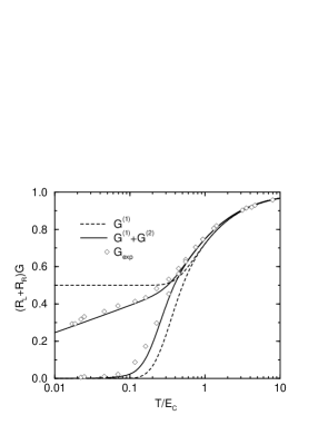
FIG. 11.: Maximal and minimal linear conductance for $E_{\rm C}=1K$ and $\alpha_{0}=0.063$. The dashed line is sequential tunneling, the solid line sequential plus cotunneling. The data points are experimental data from Ref. [16].

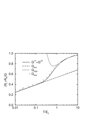
FIG. 12.: Maximal linear conductance for $E_{\rm C}=1K$ and $\alpha_{0}=0.063$. The solid line (full first plus second order result) interpolates between the long-dashed line (low-temperature expansion) and the dashed line (high-temperature expansion). The data points are experimental data from Ref. [16].

REFERENCES

• [1] D.V. Averin and K.K. Likharev, in Mesoscopic Phenomena in Solids, ed. B.L. Altshuler et al. (Elsevier, 1991).
• [2] Single Charge Tunneling, NATO ASI Series 294, H. Grabert and M.H. Devoret, eds., (Plenum Press, 1992).
• [3] G. Schön, Single-Electron Tunneling, Chapter 3 in Quantum Transport and Dissipation, T. Dittrich, P. Hänggi, G.-L. Ingold, B. Kramer, G. Schön, and W. Zwerger, (Wiley-VCH Verlag, 1998).
• [4] D.V. Averin and A.A. Odintsov, Phys. Lett. A 140, 251 (1989); D.V. Averin and Yu.V. Nazarov, Phys. Rev. Lett. 65, 2446 (1990); ibid. in Chapter 6 in Ref. [2].
• [5] L.J. Geerligs, D.V. Averin, and J.E. Mooij, Phys. Rev. Lett. 65, 3037 (1990); U. Meirav et al., Phys. Rev. Lett. 65, 771 (1990); Chapter 3,6 in Ref. [2].
• [6] H. Schoeller and G. Schön, Phys. Rev. B 50, 18436 (1994); Physica B 203, 423 (1994).
• [7] J. König, H. Schoeller, and G. Schön, Europhys. Lett. 31, 31 (1995); and in Quantum Dynamics of Submicron Structures, eds. H. A. Cerdeira et al., NATO ASI Series E, Vol. 291 (Kluwer, 1995), p.221.
• [8] J. König, H. Schoeller, and G. Schön, Phys. Rev. Lett. 78, 4482 (1997).
• [9] P. Lafarge et al., Z. Phys. B 85, 327 (1991).
• [10] K.A. Matveev, Sov. Phys. JETP 72, 892 (1991), [Zh. Eksp. Teor. Fiz. 99, 1598 (1991)].
• [11] D.S. Golubev and A.D. Zaikin, Phys. Rev. B 50, 8736 (1994).
• [12] G. Falci, G. Schön, and G.T. Zimanyi, Phys. Rev. Lett. 74, 3257 (1995).
• [13] H. Grabert, Phys. Rev. B 50, 17364 (1994).
• [14] J. König, H. Schoeller, and G. Schön, Phys. Rev. Lett. 76, 1715 (1996).
• [15] J. König, J. Schmid, H. Schoeller, and G. Schön, Phys. Rev. B 54, 16820 (1996).
• [16] P. Joyez, V. Bouchiat, D. Esteve, C. Urbina, and M.H. Devoret, Phys. Rev. Lett. 79, 1349 (1997).
• [17] The master equation is equivalent to $I(n)=I(n+1)=const.$. To determine the constant we consider the limit $n\rightarrow\infty$ and find $I(n)=0$.
• [18] Usually, the value of the integral is approximated by replacing the denominators with an $\omega$-independent term or by adding a constant finite life-time in the denominator, see e.g. Y.V. Nazarov, J. Low Temp. Phys. 90, 77 (1993); D.V. Averin, Physica 194-196, 979 (1994); P. Lafarge and D. Esteve, Phys. Rev. B 48, 14309 (1993).
• [19] D.S. Golubev and A.D. Zaikin, JETP Lett. 63, 1007 (1996), [Zh. Eksp. Teor. Fiz. Pis’ma Red. 63, 953 (1996)];
D.S. Golubev, J. König, H. Schoeller, G. Schön, and A.D. Zaikin, Phys. Rev. B 56, 15782 (1997).
• [20] G. Göppert and H. Grabert, unpublished.
Refer to caption