Coherent Resonant Tunneling Through an Artificial Molecule

Abstract

Coherent resonant tunneling through an array of quantum dots in an inhomogeneous magnetic field is investigated using an extended Hubbard model. Both the multiterminal conductance of an array of quantum dots and the persistent current of a quantum dot molecule embedded in an Aharanov-Bohm ring are calculated. The conductance and persistent current are calculated analytically for the case of a double quantum dot and numerically for larger arrays using a multi-terminal Breit-Wigner type formula, which allows for the explicit inclusion of inelastic processes. Cotunneling corrections to the persistent current are also investigated, and it is shown that the sign of the persistent current on resonance may be used to determine the spin quantum numbers of the ground state and low-lying excitated states of an artificial molecule. An inhomogeneous magnetic field is found to strongly suppress transport due to pinning of the spin-density-wave ground state of the system, and giant magnetoresistance is predicted to result from the ferromagnetic transition induced by a uniform external magnetic field.

I Introduction

Interest in the problem of coherent resonant tunneling through an interacting mesoscopic system has been stimulated by a series of elegant Aharanov-Bohm (AB) ring experiments,[1] which measured the phase of the transmission amplitude through a quantum dot in the Coulomb blockade regime. Several theoretical works have addressed the role of phase coherence in resonant tunneling through a single quantum dot: both the conductance [2] and the persistent current[3] of a quantum dot embedded in an AB ring have been calculated. Many features of the experiments of Ref. [1] have been explained by these model calculations [2, 3]; however, the correlations observed between the phases of conductance resonances rather widely separated in energy do not appear to be explicable within these simple models, and it is therefore of interest to investigate coherent resonant tunneling through complex mesoscopic systems with nontrivial substructure.

In this article, we investigate the multiterminal conductance of an artificial molecule of coupled quantum dots as well as the persistent current of an artificial molecule embedded in an AB ring. Arrays of coupled quantum dots [4, 5, 6, 7, 8, 9, 10] can be thought of as systems of artificial atoms separated by tunable tunnel barriers. The competition between intradot charge quantization effects, or Coulomb blockade,[11] due to the ultrasmall capacitance of each quantum dot to its environment, and coherent interdot tunneling has been predicted to lead to a rich spectrum of many-body effects in these systems.[12, 13, 14, 15, 16] For example, the Coulomb blockade of the individual quantum dots was predicted to be destroyed completely when interdot tunneling exceeds a critical value.[12] This phenomenon can be considered a finite-size analog of the Mott-Hubbard metal-insulator transition,[12] and has been observed experimentally in double quantum dots.[7, 10] A detailed theoretical investigation of the double quantum dot in the limit of a continuous energy spectrum on each dot, valid for very large dots, was able to describe the crossover from two isolated dots to a single, larger dot quite well.[14] An alternative approach using an effective Hubbard-like model to describe the low-lying electronic states of the double quantum dot, appropriate in the limit of a discrete energy spectrum on each dot, was also able to reproduce the experimentally observed crossover, as well as the nonlinear conductance of the system.[16] Here we will employ such an effective Hubbard model to describe coherent resonant tunneling through a one-dimensional (1D) array of quantum dots coupled to multiple leads. We will briefly consider the corresponding situation for the coherent resonant tunneling through a two-dimensional (2D) quantum dot array as well. We focus on the strongly-correlated regime, where interdot tunneling is too weak to destroy the energy gap stemming from Coulomb blockade effects, and where the energy spectrum on each dot is discrete.

An important consequence of coherent interdot tunneling in the strongly-correlated regime is the formation of interdot spin-spin correlations [17] analogous to those in a chemical bond at an energy scale $J\sim t^{2}/U$, where $U$ is the charging energy of a quantum dot and $t=(\hbar^{2}/2m^{\ast})\int d^{3}{\bf x}\,\Psi^{\ast}_{m}({\bf x})\nabla^{2}\Psi_{n}({\bf x})$ is the interdot hopping matrix element, $\Psi_{m,n}$ being electronic orbitals on nearest-neighbor dots. In a system with magnetic disorder, such a spin configuration is pinned, and the resulting blockage of spin backflow [18] leads to strong charge localization. However, an applied magnetic field will break such an antiferromagnetic bond when the Zeeman splitting $g\mu_{B}B>J$, leading to an enormous enhancement of the charge mobility. Such spin-dependent many-body effects on the magnetotransport should be experimentally observable provided $\Gamma+\Gamma^{(i)},k_{B}T\lesssim J$, where $\Gamma+\Gamma^{(i)}$ is the total broadening of the resonant levels of the system due to finite lifetime effects and inelastic scattering; they can be readily distinguished from orbital effects in arrays of quasi-two-dimensional quantum dots by applying the magnetic field in the plane of the dots. Observation of the predicted giant magnetoresistance effect in the low-temperature transport through coupled quantum dots would, we believe, represent a clear signature of the formation of an artificial molecular bond.

The paper is organized as follows: In Sec. II, an extended Hubbard model describing the low-lying electronic states of an array of coupled quantum dots is introduced, and the magnetic phase diagram of the system is discussed. In Sec. III, some general expressions for the conductance and persistent current of an interacting mesoscopic system coupled to multiple electron reservoirs are derived. In Sec. IV, the conductance through a double quantum dot in an inhomogeneous magnetic field is calculated. The magnetoresistance of the system is shown to be proportional to $U^{3}/t^{4}$. The persistent current through a double quantum dot embedded in an AB ring is also investigated. For a system with an odd number of electrons, it is shown that resonant tunneling through molecular states with odd and even $S_{z}$ leads to contributions to the persistent current of opposite signs. In Sec. V, the conductance of one-dimensional arrays of quantum dots is investigated. The inelastic scattering rate in the system is shown to be suppressed in large arrays due to the orthogonality catastrophe. A pronounced suppression of certain resonant conductance peaks in an applied magnetic field is predicted to result from a field-induced ferromagnetic transition. A many-body enhancement of localization is predicted to give rise to a giant magnetoresistance effect in systems with spin-dependent disorder. Such spin-dependent magnetoresistance effects are found to be much weaker in the ballistic transport regime. In Sec. VI the conductance in the 2D quantum dot array is investigated, and the qualitative physics is found to be similar to that in the 1D array. Some conclusions are given in Sec. VII.

II Model

The system under consideration (Fig. 1) consists of a linear array of quantum dots electrostatically defined [5, 6, 7, 8, 9] in a 2D electron gas, coupled weakly to several macroscopic electron reservoirs, with a magnetic field in the plane of the dots. Each quantum dot is modeled by a single spin-1/2 orbital, representing the electronic state nearest the Fermi energy $E_{F}$, and is coupled via tunneling to its neighbor and to one or more electron reservoirs. Transport occurs between the left (L) and right (R) reservoirs; reservoirs 1 to $N_{d}$ are considered to be ideal voltage probes,[19] and serve to introduce inelastic processes in the system.[20] Electron-electron interactions in the array are described [11, 21] by a matrix of capacitances $C_{ij}$: We assume a capacitance $C_{g}$ between each quantum dot and the system of metallic gates held at voltage $V_{g}$, an interdot capacitance $C$, and a capacitance $C_{r}$ between a quantum dot and each of its associated electron reservoirs. The diagonal elements of $C_{ij}$ are the sum of all capacitances associated with a quantum dot, $C_{11}=C_{N_{d}N_{d}}=C_{g}+C+2C_{r}$, $C_{ii}=C_{g}+2C+C_{r}$ ($1<i<N_{d}$) and the off-diagonal elements are $C_{ij}=-C$ for nearest neighbor dots $ij$. These capacitance coefficients may differ from their geometrical values due to quantum mechanical corrections, [14, 22] but enter only as parameters in our model. The Hamiltonian of the quantum dot array is

$$H_{\rm dots}=\sum_{j,\sigma}\epsilon_{j\sigma}d^{\dagger}_{j\sigma}d_{j\sigma}+\sum_{j,\sigma}\left(t_{j\sigma}d^{\dagger}_{j+1\sigma}d_{j\sigma}+\mbox{H.c.}\right)+\frac{1}{2}\sum_{i,j}(Q_{i}+Q_{g})C^{-1}_{ij}(Q_{j}+Q_{g})-\frac{Q_{g}^{2}}{2}\sum_{i,j}C_{ij}^{-1},$$ (1)

where $d^{\dagger}_{j\sigma}$ creates an electron of spin $\sigma$ in the $j$th dot, $Q_{j}\equiv-e\sum_{\sigma}d_{j\sigma}^{\dagger}d_{j\sigma}$ is the charge operator for dot $j$, $Q_{g}\equiv C_{g}V_{g}$ is a polarization charge induced by the gate, and

$$\epsilon_{j\sigma}=\epsilon_{j}+\sigma B_{j}/2-eC_{r}\sum_{i}C_{ji}^{-1}V_{i},$$ (2)

where $B_{j}$ is the Zeeman splitting on dot $j$ and $\epsilon_{j}$ is the orbital energy of the quantum-confined orbital under consideration on dot $j$. The last term in Eq. (2) represents a shift in the orbital energy due to the capacitive coupling to the reservoirs. This term has an important effect on the nonlinear transport,[23] but does not affect the linear response and equilibrium properties which are the subject of the present article. We therefore set $C_{r}=0$ in the following.

$H_{\rm dots}$ reduces to a Hubbard model [12] with on-site repulsion $U=e^{2}/C_{g}$ in the limit $C\rightarrow 0$. In general, $H_{\rm dots}$ describes an extended Hubbard model with screened long-range interactions. The elements of the inverse capacitance matrix decrease exponentially with a screening length that increases with $C/C_{g}$. For $C\ll C_{g}$, $C_{ij}^{-1}\sim(C/C_{g})^{|i-j|}/C_{g}$, while for $C/C_{g}\rightarrow\infty$, $C_{ij}^{-1}\rightarrow 1/N_{d}C_{g}$, and intradot charging effects are fully screened. Electronic correlation effects are thus decreasing functions of $C/C_{g}$. By varying the interdot electrostatic coupling, one can thus study the transition from a strongly correlated artificial molecule exhibiting collective Coulomb blockade[12] for $C\ll C_{g}$ to a ballistic nanostructure where correlation effects are negligible for $C\gg C_{g}$.

Of particular interest to us here is the magnetic phase diagram of the quantum dot array. In the strongly-correlated regime, where intradot charging is not strongly screened, the $N$-electron ground state of $H_{\rm dots}$ will form a spin-density-wave (SDW) due to interdot superexchange.[17] In an external magnetic field, the electron spins will tend to align with the field to minimize the Zeeman energy. There is thus a transition from a spin-density-wave ground state at $B=0$ to a ferromagnetic state at some critical magnetic field $B_{c}$. For an infinite 1D array with $C=0$ and $t\ll U$, one finds[24]

$$g\mu_{B}B_{c}\simeq\frac{4t^{2}}{\pi U}(2\pi n-\sin 2\pi n),$$ (3)

where $n=1-|1-N/L|$ is the filling fraction of electrons (holes) for $N<L$ ($N>L$) in the orbital under consideration. Recall that we are here considering only the single spin-1/2 orbital nearest $E_{F}$ in each quantum dot; the magnetic field required to spin-polarize an entire quantum dot is much larger.[25] In a system with $C>0$, intradot Coulomb interactions are screened, and $B_{c}$ is therefore expected to increase. Fig. 2 shows the spin susceptibility $\chi_{s}$ for $C/C_{g}=1/2$ in linear arrays with 8 electrons on 12 dots and 10 electrons on 10 dots. The $n$-dependence of $B_{c}$ in Fig. 2 is qualitatively similar to that in a system with intradot interactions only, but the values of $B_{c}$ are roughly twice those of a system with $C=0$. Note the rapid growth of $\chi_{s}$ as $B\rightarrow B_{c}$. In an infinite array, $\chi_{s}$ is expected to diverge as $B\rightarrow B_{c}$ because the system undergoes a second order quantum phase transition.[24] The spin-polarization transition (SPT) predicted to occur in an array of coupled quantum dots is in contrast to that observed in a single quantum dot, [25] where the critical point occurs for minimum total spin.

In the following, we shall investigate the effects of the SDW correlations and the SPT on the low-temperature magnetotransport through coupled quantum dots.

III Quantum Transport Formalism

Before investigating the particular Hamiltonian of interest, Eq. (1), it will first be useful to derive some general formulas for the conductance and persistent current arising due to resonant tunneling through an interacting system. An arbitrary interacting mesoscopic conductor coupled to $M$ macroscopic electron reservoirs is described by the Hamiltonian

$$H=H_{\rm int}(\{d_{n}^{\dagger},d_{n}\})+\sum_{\alpha=1}^{M}\sum_{k\in\alpha}\epsilon_{k}c_{k}^{\dagger}c_{k}+\sum_{\alpha=1}^{M}\sum_{k\in\alpha}\sum_{n}\left(V_{kn}c^{\dagger}_{k}d_{n}+{\rm H.c.}\right),$$ (4)

where $\{d^{\dagger}_{n}\}$ creates a complete set of single-particle states in the mesoscopic system, $c^{\dagger}_{k\in\alpha}$ creates an electron in state $k$ of reservoir $\alpha$, and $H_{\rm int}$ is a polynomial in $\{d^{\dagger}_{n},d_{n}\}$ which commutes with the electron number $N=\sum_{n}d^{\dagger}_{n}d_{n}$. Here the spin index $\sigma$ has been absorbed into the subscripts $n$ and $k$. We denote the ground state of $H_{\rm int}$ for each $N$ by $|0_{N}\rangle$ and the ground state energy by $E_{N}^{0}$. We assume $E_{N}^{0}$ to be nondegenerate, as is generically the case in a nonzero magnetic field.

If the tunneling barriers to the reservoirs are sufficiently large, and if the temperature and bias are small compared to the energy of an excitation, then the main effect of particle exchange with the reservoirs will be to cause transitions $|0_{N-1}\rangle\rightarrow|0_{N}\rangle$ between the nondegenerate ground states of the system. In the vicinity of such a resonance, the nonequilibrium Green’s functions describing propagation within the system in the presence of coupling to the leads can be shown to have the Breit-Wigner form[23]

$$G^{r}_{nm}(\epsilon) = \frac{\langle 0_{N-1}|d_{n}|0_{N}\rangle\langle 0_{N}|d^{\dagger}_{m}|0_{N-1}\rangle}{\epsilon-E_{N}^{0}+E_{N-1}^{0}+i\Gamma_{N}/2}+\mbox{additional poles},$$ (5)

$$G^{<}_{nm}(\epsilon) = \frac{i\langle 0_{N-1}|d_{n}|0_{N}\rangle\langle 0_{N}|d^{\dagger}_{m}|0_{N-1}\rangle\sum_{\alpha}\Gamma_{N}^{\alpha}f_{\alpha}(\epsilon)}{(\epsilon-E_{N}^{0}+E_{N-1}^{0})^{2}+(\Gamma_{N}/2)^{2}}+\mbox{additional poles},$$ (6)

where $f_{\alpha}(\epsilon)=\{\exp[(\epsilon-\mu_{\alpha})/k_{B}T]+1\}^{-1}$ is the Fermi function for reservoir $\alpha$, $\Gamma_{N}=\sum_{\alpha=1}^{M}\Gamma_{N}^{\alpha}$, and

$$\Gamma_{N}^{\alpha}=2\pi\sum_{k\in\alpha}\sum_{n,m}\langle 0_{N-1}|V_{kn}d_{n}|0_{N}\rangle\langle 0_{N}|V^{\ast}_{km}d^{\dagger}_{m}|0_{N-1}\rangle\delta(\epsilon_{k}-E_{N}^{0}+E_{N-1}^{0}).$$ (7)

Here, $G^{<,r}_{nm}(\epsilon)$ are Fourier transforms of the Keldysh Green’s function $G^{<}_{nm}(t)=i\langle d^{\dagger}_{m}(0)d_{n}(t)\rangle$ and the retarded Green’s function $G^{r}_{nm}(t)=-i\theta(t)\langle\{d_{n}(t),d^{\dagger}_{m}(0)\}\rangle$, respectively. With the aid of these Green’s functions, the conductance and persistent current resulting from resonant tunneling through the system can be calculated.

A Multiterminal Conductance Formula

The expectation value of the current flowing out of the interacting region into reservoir $\alpha$ can be expressed using the formalism of Meir and Wingreen as [26]

$$I_{\alpha}=-\frac{e}{h}\int d\epsilon\,\mbox{Im}\,\mbox{Tr}\left\{\Gamma^{\alpha}(\epsilon)\left[G^{<}(\epsilon)+2f_{\alpha}(\epsilon)G^{r}(\epsilon)\right]\right\},$$ (8)

where $\Gamma^{\alpha}_{nm}(\epsilon)=2\pi\sum_{k\in\alpha}V_{kn}V^{\ast}_{km}\delta(\epsilon-\epsilon_{k})$ is a matrix characterizing the tunnel barrier connecting reservoir $\alpha$ to the system. Inserting $G^{<,r}_{nm}$ from Eqs. (5) and (6) into Eq. (8), one finds the multiprobe current formula for resonant tunneling[23]

$$I_{\alpha}=\frac{e}{h}\sum_{\beta=1}^{M}\int d\epsilon\sum_{N}\frac{\Gamma_{N}^{\alpha}\Gamma_{N}^{\beta}\,[f_{\alpha}(\epsilon)-f_{\beta}(\epsilon)]}{\left(\epsilon-E_{N}^{0}+E_{N-1}^{0}\right)^{2}+\left(\Gamma_{N}/2\right)^{2}}.$$ (9)

The low-temperature transport through such a correlated many-body system weakly coupled to multiple leads thus exhibits resonances of the Breit-Wigner type,[20] where the positions and intrinsic widths of the resonances are determined by the many-body states of the system. Eq. (9), which expresses the current in terms of transmission probabilities, is a generalization of the multi-terminal conductance formula for a noninteracting system derived by Büttiker [27] to the case of resonant tunneling through an interacting system.

In deriving Eq. (9), we have neglected the additional poles in $G^{<,r}_{nm}(\epsilon)$, which is justified provided $k_{B}T,\,\Gamma_{N}\ll\Delta E_{N}$ and $\Delta\mu<\Delta E_{N}$, where $\Delta E_{N}=\min(E^{1}_{N}-E^{0}_{N},E^{1}_{N-1}-E^{0}_{N-1},E^{0}_{N+1}-E^{0}_{N}-\mu_{\alpha},\mu_{\alpha}-E^{0}_{N-1}+E^{0}_{N-2})$, $E^{1}_{N}$ being the energy of the lowest lying excited state of the $N$-electron system. Eq. (9) is thus appropriate to describe resonant tunneling through semiconductor nanostructures [28, 29] or ultrasmall metallic/superconducting systems [30, 31] under conditions of low temperature and bias, where transport is dominated by a single ground-state to ground-state transition $|0_{N-1}\rangle\leftrightarrow|0_{N}\rangle$. Eq. (9) is not applicable to systems with a (spin)degenerate ground state [$\Delta E(N)=0$], where the low-temperature physics is that of the Kondo effect, as discussed in Refs. [26, 32, 33, 34].

We next specialize to the configuration shown in Fig. 1. Transport occurs between the left ($L$) and right ($R$) reservoirs. The auxiliary reservoirs $1,\ldots,N_{d}$ are assumed to be connected to ideal voltmeters.[19] An ideal voltmeter should have an infinite impedance, so we demand that the expectation value of the current flowing into reservoirs $1,\ldots,N_{d}$ be zero, which fixes $\mu_{1},\ldots,\mu_{N_{d}}$ via Eq. (9). Eliminating $f_{1}(\epsilon),\ldots,f_{N_{d}}(\epsilon)$ from Eq. (9), and taking the linear response limit, one finds the effective two-terminal conductance between the left and right contacts

$$G=\frac{e^{2}}{h}\sum_{N}\frac{\Gamma_{N}^{L}\Gamma_{N}^{R}}{\Gamma_{N}^{L}+\Gamma_{N}^{R}}\int\frac{\Gamma_{N}\,[-f^{\prime}(\epsilon)]\,d\epsilon}{\left(\epsilon-E_{N}^{0}+E_{N-1}^{0}\right)^{2}+\left(\Gamma_{N}/2\right)^{2}}.$$ (10)

The total width of the $N$th resonance may be written $\Gamma_{N}=\Gamma_{N}^{L}+\Gamma_{N}^{R}+\Gamma_{N}^{(i)}$, where $\Gamma_{N}^{(i)}=\sum_{\alpha=1}^{N_{d}}\Gamma_{N}^{\alpha}$. The quantity $\Gamma_{N}^{(i)}/\hbar$ may be interpreted as the total inelastic scattering rate due to phase-breaking processes in the auxiliary reservoirs.[20] Such processes arise when an electron in the $i$th dot escapes into reservoir $i$ and is replaced by another electron from the reservoir, whose phase is uncorrelated with that of the previous electron.[20]

For simplicity, let us assume that the tunnel barriers coupling the system to the external reservoirs are described by the energy-independent parameters $2\pi\sum_{k\in\alpha}|V_{kn}|^{2}\delta(\epsilon_{k}-E)=\Gamma^{(i)}\delta_{n\alpha}$, $\alpha=1,\ldots,N_{d}$; $\Gamma\delta_{n1}$, $\alpha=L$; $\Gamma\delta_{nN_{d}}$, $\alpha=R$. Then the partial widths of the $N$th resonance are simply $\Gamma^{L}_{N}=\Gamma\sum_{\sigma}|\langle 0_{N}|d^{\dagger}_{1\sigma}|0_{N-1}\rangle|^{2}$, $\Gamma^{R}_{N}=\Gamma\sum_{\sigma}|\langle 0_{N}|d^{\dagger}_{N_{d}\sigma}|0_{N-1}\rangle|^{2}$, and

$$\Gamma_{N}^{(i)}=\Gamma^{(i)}\sum_{i=1}^{N_{d}}\sum_{\sigma}|\langle 0_{N}|d^{\dagger}_{i\sigma}|0_{N-1}\rangle|^{2}.$$ (11)

Since $\{d^{\dagger}_{i\sigma}\}$ creates a complete basis of single-particle states in the array, one would have $\Gamma_{N}^{(i)}=\Gamma^{(i)}$ for a noninteracting system. However, in an interacting system the wavefunction overlap $|\langle 0_{N}|d^{\dagger}_{i\sigma}|0_{N-1}\rangle|$ is suppressed by correlation effects, leading to an orthogonality catastrophe in the large-$N$ limit.[35] The many-body suppression of the wavefunction overlaps leads to a reduction of both the elastic broadening $\Gamma_{N}^{(e)}=\Gamma_{N}^{L}+\Gamma_{N}^{R}$ and of the inelastic broadening $\Gamma_{N}^{(i)}$ of the conductance resonances, so that the system becomes more and more weakly coupled to the environment as $N$ increases. The suppression of the wavefunction overlap with increasing $N$ is shown for an array of ten quantum dots with pure Hubbard interactions in Fig. 3. The effect of such an orthogonality catastrophe in the sequential tunneling regime has previously been discussed by Kinaret et al. [36] and by Matveev, Glazman, and Baranger. [14]

B Persistent current

Let us next consider the persistent current through the quantum dot array when the left and right reservoirs in Fig. 1(a) are connected together to form a 1D ring of length $L$ enclosing an AB flux $\Phi=(\hbar c/e)\phi$. Since the persistent current is an equilibrium property, the auxiliary reservoirs must be in mutual equilibrium at electrochemical potential $\mu$, as indicated in Fig. 1(b). The persistent current in such an open system is given by $I(\phi)=-(e/\hbar)\partial\Omega/\partial\phi$, where $\Omega$ is the grand canonical potential. The grand canonical potential may be determined from the electronic scattering matrix of the system, as discussed by Dashen, Ma, and Bernstein [37] and by Akkermans et al.,[38] and is

$$\Omega(\phi)=-\int\frac{dE}{2\pi}f(E)\,\mbox{Im}\ln\det S(E,\phi),$$ (12)

where $S(E,\phi)$ is the scattering matrix of the multiply-connected structure shown in Fig. 1(b) and $f(E)$ is the Fermi function with electrochemical potential $\mu$. In order to obtain $S(E,\phi)$, it is useful first to introduce the scattering matrix $S(E)$ for the structure shown in Fig. 1(a), which is related simply to the retarded Green’s function,

$$S_{kk^{\prime}}(E)=-\delta_{kk^{\prime}}+2\pi i\sum_{nm}\frac{V_{km}^{\ast}V_{k^{\prime}n}}{\sqrt{v_{k}v_{k^{\prime}}}}G^{r}_{nm}(E),$$ (13)

where $v_{k\in\alpha}$ is the group velocity of state $k$ in reservoir $\alpha$. Using Eq. (5), one sees that $S(E)$ has the Breit-Wigner form discussed by Büttiker.[20] $S(E)$ may be divided into submatrices $r_{kk^{\prime}}$, describing reflection of mode $k^{\prime}$ in the reservoir back into mode $k$ in the reservoir, $\varepsilon_{k}$ and $\delta_{k}$, describing transmission of mode $k$ from the reservoir into the the ring to the left and right, respectively, $\gamma$, describing transmission of a circulating state in the ring through the quantum dot array, and $\alpha$ and $\beta$, describing reflection of the circulating states in the ring at the left and right ends of the quantum dot array, respectively. In terms of the submatrices of $S(E)$, the flux-dependent scattering matrix for the combined structure may be written

$$S_{kk^{\prime}}(E,\phi)=r_{kk^{\prime}}+\frac{\alpha\delta_{k}\delta_{k^{\prime}}+\beta\varepsilon_{k}\varepsilon_{k^{\prime}}-(\gamma-\cos\phi e^{-ipL})(\varepsilon_{k}\delta_{k^{\prime}}+\delta_{k}\varepsilon_{k^{\prime}})}{\gamma^{2}-\alpha\beta-2\gamma\cos\phi e^{-ipL}+e^{-2ipL}},$$ (14)

where $p=\sqrt{2mE}/\hbar$ and it is assumed that $\epsilon_{k}=\epsilon_{k^{\prime}}=E$. Substituting Eq. (14) into Eq. (12), and taking the derivative with respect to $\phi$, one obtains the persistent current due to coherent resonant tunneling through the quantum dot array. The general expression for $I(\phi)$ is somewhat cumbersome, but for the special case $\Gamma_{N}^{L}=\Gamma_{N}^{R}=\Gamma_{N}^{(e)}/2$, one finds the simple result

$$I(\phi)=\frac{e\Gamma_{N}^{(e)}}{2h}\int\frac{dE\,f(E)\,\Gamma_{N}^{(i)}\frac{\textstyle\sin\phi\sin pL}{\textstyle(\cos\phi-\cos pL)^{2}}}{\left[E-E_{N}^{0}+E_{N-1}^{0}-\frac{(\Gamma_{N}^{(e)}/2)\sin pL}{\cos pL-\cos\phi}\right]^{2}+\left(\Gamma_{N}^{(i)}/2\right)^{2}}.$$ (15)

The persistent current is thus also determined by the conductance matrix elements $\Gamma_{N}^{\alpha}$. From Eq. (15) one sees that as the energy of the resonance is tuned through the Fermi level (by varying the gate voltage $V_{g}$), the persistent current exhibits a maximum of height $\mbox{}\sim(e\Gamma_{N}^{(e)}/\hbar)\sin\phi\sin k_{F}L$, which decays with a width $\Gamma_{N}$ when the resonance is moved above $\mu$. $I$ also decays when the resonance is moved below the Fermi level, but in an oscillatory pattern determined by the level spacing in the ring.

In the limit $\Gamma_{N}^{(i)}\rightarrow 0$ (closed system), the integrand in Eq. (15) consists of a series of delta functions whose weights give the current contributed by each of the discrete states in the ring which couple to the dot array, subject to periodic boundary conditions. If the ring has dimensions comparable to those of the dot array, then the level spacing in the ring may exceed the width of the resonance ($\hbar v_{F}/L>\Gamma_{N}$), and the above approach will break down. The persistent current will then be dominated by charge fluctuations coupling the highest occupied state in the ring, of energy $\epsilon_{F}$, with the lowest unoccupied many-body state in the dotarray.[3] The coupling matrix element is

$$|t|^{2}=t_{R}^{2}+t_{L}^{2}+2t_{R}t_{L}\cos\phi,$$ (16)

where the matrix elements

$$t_{L} = \sum_{\sigma}\langle 0_{N}|V_{k_{F}1}d^{\dagger}_{1\sigma}|0_{N-1}\rangle$$ (17)

$$t_{R} = \sum_{\sigma}\langle 0_{N}|V_{k_{F}N_{d}}d^{\dagger}_{N_{d}\sigma}|0_{N-1}\rangle$$ (18)

may be chosen real. A straightforward calculation[3] then yields the persistent current through the quantum dot array

$$I(\phi)=-\frac{2(e/\hbar)t_{R}t_{L}\sin\phi}{[(\epsilon_{F}-E_{N}^{0}+E_{N-1}^{0})^{2}+4|t|^{2}]^{1/2}}.$$ (19)

The product $t_{R}t_{L}$ may be greater or less than zero depending on the relative signs of $V_{k_{F}1}$ and $V_{k_{F}N_{d}}$, and on the relative signs of the wavefunction overlaps, so the persistent current on resonance may be either diamagnetic or paramagnetic. For a purely 1D system of spinless electrons, or with an even number of spin-1/2 electrons, the sign of $I(\phi)$ is determined by the total number of electrons in the system, as discussed in Ref. [3]. This is a manifestation of the so-called Leggett theorem.[39] However, in general the sign of $I(\phi)$ depends on the particular state which dominates the resonance, and may be used to classify the quantum numbers of that state, as discussed below.

IV Double Quantum Dot

Let us first consider the case of double quantum dot, for which the conductance matrix elements (7) can be obtained analytically. For $N_{d}=2$, $H_{\rm dots}$ reduces to a two-site Hubbard model with on-site repulsion $U=e^{2}C_{\Sigma}/(C_{\Sigma}^{2}-C^{2})$ and nearest neighbor repulsion $U_{12}=e^{2}C/(C_{\Sigma}^{2}-C^{2})$, where $C_{\Sigma}=C_{g}+C+2C_{r}$. Spin disorder is introduced via a Zeeman splitting on dot 1, $B_{1}=4t\Delta$, $B_{2}=0$. Experimentally, such an inhomogeneous field could be produced, e.g., by the presence of a small ferromagnetic particle. The total width of the one-particle resonance is found to be $\Gamma_{1}=\Gamma+\Gamma^{(i)}$, and the prefactor in Eq. (10) is $\Gamma_{1}^{L}\Gamma_{1}^{R}/(\Gamma_{1}^{L}+\Gamma_{1}^{R})=(\Gamma/4)/(1+\Delta^{2})\equiv\Gamma_{0}$. The maximum conductance at the one-particle resonance is thus

$$G_{1}^{*} = \frac{\textstyle e^{2}/h}{\textstyle(1+\Delta^{2})(1+\Gamma^{(i)}/\Gamma)},\;\;\;\;\;\;\;T=0$$ (20)

$$= e^{2}\Gamma_{0}/4\hbar k_{B}T,\;\;\;\Gamma+\Gamma^{(i)}\ll k_{B}T\ll t\sqrt{1+\Delta^{2}}.$$ (21)

Inelastic scattering suppresses the resonant conductance at $T=0$, but has no effect when the resonance is thermally broadened. For $U-U_{12}\gg t$, the two-particle ground state of the double quantum dot has an antiferromagnetic spin configuration characterized by the superexchange parameter

$$J=2t\left(\gamma-\Delta+\sqrt{\gamma^{2}+\Delta^{2}}\right),$$ (22)

where $\gamma=t/(U-U_{12})$. Note that $2t\gamma\leq J\leq 4t\gamma$. The two-particle resonance is separated from the one-particle resonance by $e\Delta Q_{g}/(C_{\Sigma}-C)=U_{12}+2t(1+\Delta^{2})^{1/2}-J$, and the conductance is determined by the matrix elements

$$\langle 0_{2}|d^{\dagger}_{j\uparrow}|0_{1}\rangle=\frac{\sqrt{2}}{A}\left\{\frac{2\gamma}{\left[1+\left(\Delta\mp\sqrt{\Delta^{2}+1}\right)^{2}\right]^{1/2}}+\frac{1\mp\Delta/\left(\gamma+\sqrt{\gamma^{2}+\Delta^{2}}\right)}{\left[1+\left(\Delta\pm\sqrt{\Delta^{2}+1}\right)^{2}\right]^{1/2}}\right\},$$ (23)

where $A^{2}=1+\Delta^{2}/(\gamma+\sqrt{\gamma^{2}+\Delta^{2}})^{2}$ and the upper (lower) sign holds for $j=1$ (2). For $B_{1}\gtrsim J$, the antiferromagnetic spin configuration is pinned, leading to a strong suppression of the amplitude to inject electron 2 into dot 1, and a concommitant suppression of the second conductance peak. Inserting Eq. (23) into Eqs. (7) and (10), one finds the $T=0$ resonant conductance

$$G_{2}^{*} = 16(e^{2}/h)(\gamma/\Delta)^{2}/(1+\Gamma^{(i)}/\Gamma),\;\;\;\;\;\;\gamma\ll\Delta\ll 1$$ (24)

$$= 4(e^{2}/h)\gamma^{2}/(1+\Gamma^{(i)}/\Gamma),\;\;\;\;\;\;\Delta\gg 1.$$ (25)

A second doublet of conductance peaks for $N=3,\,4$ is separated from this doublet by $\Delta Q_{g}\simeq e$ (center to center), and one finds $G_{3}^{*}=G_{2}^{*}$, $G_{4}^{*}=G_{1}^{*}$ due to electron-hole symmetry. The resonant conductance for $N=2$ is suppressed by a factor of $\gamma^{2}$ compared to that for $N=1$ due to collective spin pinning (one readily verifies that the resonant conductance is suppressed by the same many-body factor in the regime of thermally broadened resonances). This dramatic many-body suppression of the conductance is illustrated in Fig. 4 for several values of $\gamma$. The effect of spin disorder is to be contrasted with that of a charge detuning $\Delta=(\epsilon_{1}-\epsilon_{2})/2t$, investigated by Klimeck et al. [13] and by van der Vaart et al.,[6] for which both $G_{1}^{*}$ and $G_{2}^{*}$ are given by Eq. (21) at $T=0$ ($G_{2}^{*}$ is then reduced by a factor of 2 in the thermally broadened regime). The very different effects of spin and charge disorder stem from the fact that the repulsive interactions in Eq. (1) enhance spin-density fluctuations, but suppress charge-density fluctuations.

Let us now consider the effect of an additional homogeneous magnetic field applied parallel to the inhomogeneous field, $B_{1}=4t\Delta+B$, $B_{2}=B$. For $B>J$, it is energetically favorable to break the antiferromagnetic bond between the dots and form a spin-polarized state, thus preventing collective spin pinning effects. $G_{2}^{*}$ is then given by Eq. (21). The resulting magnetoresistance on resonance for $T=0$ and $\Delta\gg 1$ is thus

$$\frac{\Delta R^{*}}{\Delta B}=-\frac{h}{e^{2}}\frac{g\mu_{B}}{4J\gamma^{2}}(1+\Gamma^{(i)}/\Gamma)\sim-\frac{h}{e^{2}}\frac{g\mu_{B}(U-U_{12})^{3}}{8t^{4}}.$$ (26)

In the thermally broadened resonance regime, the factor $(1+\Gamma^{(i)}/\Gamma)$ is replaced by $2k_{B}T/\pi\Gamma$. Since the Coulomb energy $U-U_{12}$ is typically large compared to the interdot tunneling matrix element $t$, the predicted magnetoresistance is extremely large. This giant magnetoresistance effect is a direct indication of the field-induced breaking of the artificial molecular bond between the dots. [40]

The conditions necessary to observe the predicted magnetoresistance effect may be determined by including the effect of transport through the triplet excited state via the method of Refs. [11] and [13]. One finds the resonant conductance at $B=0$ for $k_{B}T\gg\Gamma+\Gamma^{(i)}$

$$G_{2}^{*}=\frac{e^{2}}{2\hbar k_{B}T}\frac{\exp(\beta J)}{2\exp(\beta J)-1}\left(\Gamma_{s}+\frac{2\Gamma_{t}}{\exp(\beta J)+1}\right),$$ (27)

where $\Gamma_{s}\simeq 4\gamma^{2}\Gamma$ is the sequential tunneling rate through the pinned antiferromagnetic ground state and $\Gamma_{t}=\Gamma_{0}$ is the sequential tunneling rate through the triplet excited state. The magnetoresistance is thus reduced by a factor of 2 at a temperature $k_{B}T_{1/2}=J/\ln(\Gamma_{t}/\Gamma_{s})$. Increased coupling to the leads and/or inelastic scattering can be shown to lead to a similar admixture of transport through excited states when $\Gamma+\Gamma^{(i)}\sim J$. We therefore expect the predicted giant magnetoresistance effect to be observable for $k_{B}T,\,\Gamma+\Gamma^{(i)}\lesssim J$. In currently available GaAs quantum dot systems, charging energies are typically of order 1meV, and one expects tunneling matrix elements $t\sim 0.1\mbox{meV}$ for moderate to strong interdot tunneling, so values of $J$ in the range .01—0.1meV should be attainable.

Let us next consider the persistent current through the double quantum dot. From Eqs. (15) and (19), one sees that the persistent current is also suppressed at the $N=2$ resonance due to the many-body factor (23). However, in the later case of a nanoscopic ring with level spacing $\hbar v_{F}/L\gg\Gamma_{2}$, the suppression of the persistent current is only linear in $\langle 0_{2}|d^{\dagger}_{j\uparrow}|0_{1}\rangle$. An interesting question is the effect of cotunneling through excited states of the double dot when the dot ring-coupling $|t|$ exceeds the many-body level spacing in the double dot $J$. In order to address this question, we have studied the closed system of a double quantum dot embedded in an AB ring numerically using the Lanczos technique[41] (see Fig. 5). The Hilbert space was truncated by discretizing the ring (8 sites were used). In order to distinguish the contributions from tunneling through the $S_{z}=0$ ground state and the $S_{z}=1$ excited state of the double dot, the total number of electrons in the system was chosen to be odd (in this case 5). Thus if the total number of up-spin electrons $N_{\uparrow}$ is even, the total number of down-spin electrons $N_{\downarrow}$ must be odd, and vice versa.[42] In the weak-coupling limit $|t|\ll J$, where a single level of the double dot contributes to the resonant current, the spin of the tunneling electron is well defined, and is

$$\hbar\sigma/2=\langle 0_{N}|S_{z}|0_{N}\rangle-\langle 0_{N-1}|S_{z}|0_{N-1}\rangle.$$ (28)

Fig. 5 shows the persistent current at $\phi=\pi/2$ as a function of the gate voltage $Q_{g}$ in the vicinity of the first Coulomb blockade doublet centered near $Q_{g}=e/2$. The doublet splitting is here enhanced due to the finite level spacing in the ring. For $\Delta>0$, the ground state of the coupled dot-ring system generally has $N_{\downarrow}=N_{\uparrow}+1$ (in this case $N_{\downarrow}=3$ and $N_{\uparrow}=2$). The first electron to enter the double dot as $Q_{g}$ is increased from zero enters the lowest single-electron eigenstate of the double dot, and thus has $\sigma=-1$. Since $N_{\downarrow}$ is odd, the resonant current is diamagnetic due to the parity effect.[3] The second electron to enter the double dot goes into the state $|0_{2}\rangle$ and thus has $\sigma=+1$. Since $N_{\uparrow}$ is even, the resonant current is thus paramagnetic[3] (see solid curve in Fig. 5). The height of the second peak is reduced compared to that of the first, but by a smaller factor than for the conductance [c.f., Eqs. (10) and (19)]. However, there is also a contribution to the persistent current due to cotunneling through the first excited state of the double dot, which is higher in energy by $J$ than $|0_{2}\rangle$. This state has $\sigma=-1$, and thus leads to a diamagnetic contribution to $I(\phi)$. This state couples more strongly to the leads, but is suppressed by a large energy denominator when $|t|\ll J$. As $|t|$ is increased (dotted and dashed curves in Fig. 5), the cotunneling contribution becomes increasingly important, and there is a crossover from a small paramagnetic peak to a larger diamagnetic peak for $|t|>J$. Fig. 5 clearly shows that the sign of the persistent current induced by tunneling through a 1D structure may be used to characterize the spin quantum numbers of the ground state and low-lying excited states of such a system.

V 1D Array of Quantum Dots

Let us next consider tunneling through larger arrays of quantum dots. For $N_{d}>2$, the $N$-body ground states of Eq. (1) were obtained by the Lanczos technique,[41] and the conductance was calculated using Eq. (10). At $T=0$ and in the absence of inelastic scattering, the conductance peaks all have height $e^{2}/h$ in the absence of disorder, since in that case $\Gamma_{N}^{R}=\Gamma_{N}^{L}=\Gamma_{N}/2$. Inelastic scattering leads to additional broadening of the conductance peaks, and suppression of the resonant conductance below $e^{2}/h$. Disorder also leads to a suppression of the $T=0$ resonant conductance below $e^{2}/h$ due to the breaking of left-right symmetry $\Gamma_{N}^{R}\neq\Gamma_{N}^{L}$. In the following, we concentrate on the thermally broadened resonance regime, where the peak heights of the conductance resonances depend most strongly on the conductance matrix elements $\Gamma_{N}^{L}$ and $\Gamma_{N}^{R}$. For $k_{B}T\gg\Gamma_{N}$, Eq. (10) simplifies to [11, 13]

$$G=\frac{e^{2}}{h}\sum_{N}\frac{\Gamma_{N}^{L}\Gamma_{N}^{R}}{\Gamma_{N}^{L}+\Gamma_{N}^{R}}[-f^{\prime}(\mu-E_{N}^{0}+E_{N-1}^{0})].$$ (29)

Fig. 6 shows the conductance through a linear array of 10 quantum dots with $C=0$ as a function of the chemical potential $\mu$ in the leads, whose value relative to the energy of the array is controlled by the gate voltages. The two Coulomb blockade peaks in Fig. 6 are split into multiplets of 10 by interdot tunneling, as discussed in Refs. [12, 13] We refer to these multiplets as Hubbard minibands. The energy gap between multiplets is caused by collective Coulomb blockade,[12] and is analogous to the energy gap in a Mott insulator.[43] The heights of the resonant conductance peaks in Fig. 6(a) can be understood as follows: Since the barriers to the leads are assumed to be large, the single-particle wavefunctions of the array are like those of a particle in a one-dimensional box. The lowest eigenstate has a maximum in the center of the array and a long wavelength, hence a small amplitude on the end dots, leading to a suppression of the 1st conductance peak. Higher energy single-particle states have shorter wavelengths, and hence larger amplitudes on the end dots, leading to conductance peaks of increasing height. The suppression of the conductance peaks at the top of the 1st miniband can be understood by an analogous argument in terms of many-body eigenstates; the 10th electron which enters the array can be thought of as filling a single hole in a Mott insulator, etc.

In Fig. 6(b), the spin-degeneracy of the quantum dot orbitals is lifted by the Zeeman splitting. There is a critical field $B_{c}$ above which the system is spin-polarized [c.f., Eq. (3)] Because $B_{c}$ is a function of $n$, one can pass through this spin-polarization transition (SPT) by varying $n$ at fixed $B$. In Fig. 6(b), this transition occurs between the 4th and 5th electrons added to the array, consistent with the prediction of Eq. (3). The effect of this transition on the conductance spectrum is dramatic: The first 4 electrons which enter the array have spin aligned with $B$ (up), but the 5th electron enters with the opposite spin, and goes predominantly into the lowest single-particle eigenstate for down-spin electrons, which couples only weakly to the leads, leading to a suppression of the 5th resonant conductance peak by over an order of magnitude. It should be emphasized that the heights of the conductance peaks change discontinuously as a function of $B$ each time there is a spin-flip.

Splitting of the Coulomb blockade peaks due to interdot coupling and suppression of the conductance peaks at the miniband edges have recently been observed experimentally by Waugh et al. [7] However, it has been pointed out [7] that both effects can also be accounted for by a model [21] of capacitively coupled dots with completely incoherent interdot tunneling. It is therefore of interest to consider the effects of interdot capacitive coupling in the regime of coherent interdot transport. A nonzero interdot capacitance $C$ introduces long-range electron-electron interactions in Eq. (1) and decreases the intradot charging energy $U$. Fig. 2 shows the spin susceptibility $\chi_{s}$ for $C/C_{g}=1/2$ in linear arrays with 8 electrons on 12 dots and 10 electrons on 10 dots. The $n$-dependence of $B_{c}$ in Fig. 2 is qualitatively similar to that in a system with intradot interactions only, but the values of $B_{c}$ are roughly twice those of a system with $C=0$. Note the rapid growth of $\chi_{s}$ as $B\rightarrow B_{c}$. In an infinite array, $\chi_{s}$ is expected to diverge as $B\rightarrow B_{c}$ because the system undergoes a second order quantum phase transition. [24] The SPT predicted to occur in an array of coupled quantum dots is in contrast to that observed in a single quantum dot, [25] where the critical point occurs for minimum total spin.

Disorder introduces a length scale which cuts off the critical behavior as $B\rightarrow B_{c}$. However, as shown in Fig. 7, where disorder $\delta t\sim t$ has been included in the hopping matrix elements, the SPT has a clear signature in the magnetotransport even in a strongly disordered system. In Fig. 7, the peak splitting due to capacitive coupling is roughly ten times that due to interdot tunneling, so that the peak positions are within $\sim 10\%$ of those predicted by a classical charging model.[21] However, the dramatic dependence of peak heights on magnetic field—the 4th conductance peak in Fig. 7(b) is suppressed by a factor of 32 compared to its $B=0$ value due to the density-dependent SPT described above—can not be accounted for in a model which neglects coherent interdot tunneling. This effect should be observable provided $g\mu_{B}B_{c}>\mbox{max}(k_{B}T,\hbar/\tau_{i})$, where $\tau_{i}$ is the inelastic scattering time. We believe that this striking magnetotransport effect is the clearest possible signature of a coherent molecular wavefunction in an array of quantum dots.

Fig. 8 shows the conductance spectrum for an array of 6 quantum dots with the same parameters as in Fig. 7, but with spin-dependent disorder in the hopping matrix elements, as could be introduced by magnetic impurities. Several conductance peaks at $B=0$ (solid curve) are strongly suppressed due to a many-body enhancement of localization. This effect arises because repulsive on-site interactions enhance spin-density wave correlations, which are pinned by the spin-dependent disorder.[45] At $B=1.3\mbox{T}$ (dotted curve) the system is above $B_{c}$ and is spin-polarized, circumventing this effect. The second conductance peak is enhanced by a factor of 1600 at 1.3T compared to its size at $B=0$ (not visible on this scale). This giant magnetoconductance effect is a many-body effect intrinsic to the regime of coherent interdot transport.

Another interesting phenomenon stemming from the competition between coherent interdot tunneling and charging effects is the Mott-Hubbard metal-insulator transition (MH-MIT), which occurs when collective Coulomb blockade (CCB) [12] is destroyed due to strong interdot coupling. For GaAs quantum dots larger than about 100nm in diameter, we find that this transition is caused by the divergence of the effective interdot capacitance, similar to the breakdown of Coulomb blockade in a single quantum dot.[44] Within the framework of the scaling theory of the MH-MIT, [43] one expects a crossover from CCB to ballistic transport in a finite array of quantum dots when the correlation length $\xi$ in the CCB phase significantly exceeds the linear dimension $L$ of the array. Fig. 9 shows the conductance spectrum for 5 quantum dots with 5 spin-1/2 orbitals per dot. The divergence of the effective interdot capacitance as the interdot barriers become transparent is simulated by setting $C^{(n)}/C_{g}=2^{n-1}$, $n=0,\ldots,4$. In Fig. 9, minibands arising from each orbital are split symmetrically into multiplets of 5 peaks by CCB, with the center to center spacing between multiplets equal to $e^{2}/C_{g}$, while the energy gap between minibands corresponds to the band gap $\sim\,\Delta$ enhanced by charging effects. The CCB energy gap is evident in the first 3 minibands, but is not resolvable for the higher orbitals ($C/C_{g}\geq 4$), although there is still a slight suppression of the conductance peaks near the center of the 4th miniband. Comparison of the compressibility of the system to a universal scaling function for the MH-MIT calculated by the method of Ref. [43] indicates $\xi/L\sim 10^{3}$ for $C/C_{g}=8$, so that the transport in the 5th miniband is effectively ballistic. The peak spacing within a miniband saturates at $e^{2}/LC_{g}$ (plus quantum corrections $\sim t/L$) in the ballistic phase because the array behaves like one large capacitor, as observed experimentally in Ref. [7]. Fig. 9(b) shows the effects of a magnetic field on the conductance spectrum: a sequence of SPTs is evident in the different minibands, with $B_{c}$ an increasing function of $C/C_{g}$, leading to quenching of magnetoconductance effects in the ballistic regime.

A finite-size scaling analysis of the compressibility indicates that the MH-MIT probably occurs at $C/Cg=\infty$ in an infinite array of quantum dots, when the interdot barriers become transparent to one transmission mode.[46]

VI 2D array of quantum dots

Finally, we briefly consider coherent tunneling through a 2D quantum dot array (Fig. 10) to investigate whether the many-body giant magnetoconductance effect discussed in Sec. V arises in two dimensions as well. We use Eq. (29) to calculate the linear tunneling conductance through a 2D $3\times 3$ quantum dot array consisting of $N_{d}=9$ quantum dots. The corner dots in the array are weakly coupled to electron reservoirs as shown in Fig. 10. The Hamiltonian of the array is the same as that given by Eq. (1), where the second term is now modified to incorporate the nearest neighbor tunneling in the 2D array: the tunneling amplitudes connecting two nearest neighbor dots $i$ and $j$ in the array are multiplied by the Peierls phase factors $e^{i\frac{e}{\hbar}\int_{ij}\vec{A}\cdot\vec{dl_{ij}}}$ with $\vec{A}$ as the magnetic vector potential.[47] We consider a uniform flux $\phi=Ba^{2}$ piercing each unit cell of the array in Fig. 10. The magnetic field $B$ enters through the tunneling amplitudes $t_{ij}$ and through the intradot single-particle field dependence entering $\varepsilon_{i\sigma}$ in Eq. (2). The flux sensitive phase factors in Eq. (1) lead to a flux periodic modulation of the linear conductance with periodicity given by one fundamental flux unit $hc/e$. This flux dependence of the linear conductance and the associated ground state persistent current oscillations have been discussed elsewhere.[47] Here we follow our discussion in the previous section, concentrating on a fixed applied field, and focus on the magnetic field induced spin effect (i.e. the single-dot Zeeman physics) on the linear conductance peak heights in the $3\times 3$ array.

The partial width $\Gamma_{N}^{L}$ of the $N$th resonance is plotted as a function of $N$ in Fig. 11 (a) and (b) for the applied magnetic field $B=0$ and $B=1.3$T in the array, respectively. The corresponding linear conductance in the $3\times 3$ array is shown in Fig. 12. The peak splittings in the linear conductance in the $3\times 3$ array are not distributed uniformly, but the shape of the envelope function for conductance peak heights is similar to that in 1D chains (e.g. compare Figs. 6 and 12). This envelope function is peaked at quarter filling in the Hubbard model we use here. In the strongly correlated Hubbard array, the overlap matrix element is approximately given by $\Gamma_{N}^{L}\sim[1-P_{N-1}(1)]P_{N}(1)$ with $P_{N}(1)=\sum_{\sigma}\langle 0_{N}|d_{1\sigma}^{\dagger}d_{1\sigma}|0_{N}\rangle$ being the probability to find the corner dot occupied. For $U/t=10$, the maximum and minimum $P_{N}(1)$ are approximately 1 and 0, leading to a peak in the linear conductance at quarter filling (and also at three quarter filling due to particle-hole symmetry) in Hubbard arrays. The addition spectra shown in the conductance vs. chemical potential plots of Figs. 11 and 12 correspond to a sequence of ground states that are characterized by the number of electrons $N$, the total spin $S$, and the component $S_{z}$ of the total spin along the quantization axis. The ground state $(N,S,S_{z})$ sequence for $B=0$ in the array is $(1,1/2,1/2)\rightarrow(2,0,0)\rightarrow(3,3/2,1/2)\rightarrow(4,1,1)\rightarrow(5,1/2,1/2)\rightarrow(6,0,0)\rightarrow(7,1/2,1/2)\rightarrow(8,0,0)\rightarrow(9,1/2,1/2)$. In the $B=1.3$T array the similar sequence of the ground states is given by $(1,1/2,1/2)\rightarrow(2,1,1)\rightarrow(3,3/2,3/2)\rightarrow(4,2,2)\rightarrow(5,5/2,5/2)\rightarrow(6,2,2)\rightarrow(7,1/2,1/2)\rightarrow(8,1,1)\rightarrow(9,1/2,1/2)$. It can be seen from the latter sequence that the $6$th linear conductance peak at $B=1.3$ is suppressed (by a factor of 23) due to the spin polarization transition discussed in the previous section for 1D arrays. It can also be seen that the transition from the $6$-electron to $7$-electron ground state is forbidden at $B=1.3T$ and therefore the $7$th peak is absent in Figs. 11(b) and 12(b). This is an example of the so-called “spin-blockade” phenomenon.[48] The $8$th peak at $B=0$ in the array is present in the conductance and partial width traces in Figs. 11(a) and 12(a), although it is suppressed by a factor of approximately 100. Finally, for $N=1$ the charge density on the corner dots is 10 times smaller at $B=1.3$T, leading to the suppression of the first peak at $B=1.3$T from its $B=0$ value in Fig. 11.

We conclude that the spin polarization transition discussed in Sec. V for the case of the 1D array leads to a similar suppression of the linear conductance peak heights in 2D arrays of quantum dots.

VII Conclusions

We have shown that the formation of artificial molecular bonds due to interdot superexchange can drastically modify the low-temperature transport through coupled quantum dots. The resulting interdot spin-density-wave (SDW) correlations are strongly pinned by magnetic disorder, leading to a suppression of transport. These SDW correlations are destroyed in an applied magnetic field large enough to polarize all the electron spins, leading to a marked increase of the conductance at the spin-polarization transition (SPT). For a double quantum dot, this leads to a magnetoresistance proportional to $(g\mu_{B}h/e^{2})U^{3}/t^{4}$, where $U$ is the charging energy of a quantum dot and $t$ is the interdot hopping matrix element. Since $U$ is typically at least an order of magnitude greater than $t$, we have termed this effect giant magnetoresistance. For larger 1D arrays of quantum dots, the magnetoresistance was found to be proportional to $(g\mu_{B}h/e^{2})U^{2N-1}/t^{2N}$ at the $N$-electron resonance when $N$ is even, while saturating to a smaller, $N$-independent value for $N$ odd. This $U$-dependence reflects the probability of an electron to tunnel all the way through the system while leaving the pinned, Néel ordered spin configuration of the ground state undisturbed. The giant magnetoresistance effect proposed here for coupled quantum dots is expected to be quite generic in quasi-one-dimensional systems with magnetic disorder.

In addition to the giant magnetoresistance effect predicted for 1D arrays of quantum dots with magnetic disorder, the SPT was shown to lead to large magnetoresistance effects in non-disordered 1D and 2D systems and in systems with charge disorder. These many-body effects are likely to provide a fruitful area of research in the next generation of coupled semiconductor quantum dot systems.

ACKNOWLEDGMENTS

This work was supported by the U.S. Office of Naval Research.

 

 

FIG. 1.: (a) Schematic diagram of a linear array of quantum dots. (b) A quantum dot array embedded in an Aharanov-Bohm ring, formed by connecting the left and right reservoirs in (a).

 

FIG. 2.: Spin susceptibility $\chi_{s}=\hbar^{-1}\Delta S/\Delta B$ at $T=0$ vs. magnetic field $B$ for linear arrays of GaAs quantum dots with $e^{2}/C_{g}=1\mbox{meV}$, $C/C_{g}=0.5$, and $t=.05\mbox{meV}$. Squares: 10 electrons on 10 dots ($B_{c}\approx 1.5\mbox{T}$); triangles: 8 electrons on 12 dots ($B_{c}\approx 1\mbox{T}$).

 

FIG. 3.: The total wavefunction overlap $\Gamma_{N}^{(i)}/\Gamma^{(i)}=\sum_{i=1}^{N_{d}}\sum_{\sigma}|\langle 0_{N}|d^{\dagger}_{i\sigma}|0_{N-1}\rangle|^{2}$ as a function of $N$ for an array of ten quantum dots with pure Hubbard interactions $U=10t$. The $x$ coordinate of the $N$th peak indicates the value of the polarization charge $Q_{g}=C_{g}V_{g}$ at which the $N$th electron is added to the system. The suppression of $\Gamma_{N}^{(i)}$ with increasing $N$ is evident in the lower Hubbard band $Q_{g}/e<1$. The symmetry about $Q_{g}/e=1$ follows from the particle-hole symmetry of Eq. (1)

 

FIG. 4.: Resonant conductance at $T=0$ in units of $(e^{2}/h)/(1+\Gamma^{(i)}/\Gamma)$ as a function of the Zeeman splitting on dot 1 for $\gamma^{-1}=0$, 3, 10, 30 (top to bottom). If an additional uniform external field $B>J$ is applied, the conductance is restored to the value for $\gamma^{-1}=0$, leading to giant magnetoresistance.

 

FIG. 5.: Persistent current through a double quantum dot embedded in an Aharanov-Bohm ring as a function of the gate voltage. Here $t=1$, $U=10$, $U_{12}=0$, and $V_{k1}=V_{kN_{d}}=V$. The current is expressed in units of $I_{\ast}=eV/2^{1/2}\hbar$, the value on resonance in the absence of correlations and asymmetry. Solid curve: $V=1/32$; dotted curve: $V=1/8$; dashed curve: $V=1/2$.

 

FIG. 6.: Conductance vs. chemical potential $\mu$ through a linear array of 10 GaAs quantum dots with one spin-1/2 orbital per dot. $e^{2}/C_{g}=1\mbox{meV}$, $C=0$, $t=0.1\mbox{meV}$, and $T=35\mbox{mK}$. Splitting of the two Coulomb blockade peaks into minibands is driven by $t$. The suppression of the 5th peak in (b) is the result of a density-dependent SPT.

 

FIG. 7.: Conductance vs. chemical potential $\mu$ through a linear array of 6 GaAs quantum dots with one spin-1/2 orbital per dot. $e^{2}/C_{g}=1\mbox{meV}$, $C/C_{g}=0.5$, $\bar{t}=.05\mbox{meV}$, $T=120\mbox{mK}$. Disorder $\delta t/\bar{t}\sim 1$ ($t_{i\uparrow}=t_{i\downarrow}$) is present in the hopping matrix elements. The splitting of the Coulomb blockade peaks into multiplets is dominated by $C$; however, the effect of $B$ is similar to that in Fig. 1.

 

FIG. 8.: Conductance vs. chemical potential $\mu$ through a linear array of 6 GaAs quantum dots with one spin-1/2 orbital per dot. $e^{2}/C_{g}=1\mbox{meV}$, $C/C_{g}=0.5$, $\bar{t}=.05\mbox{meV}$, $T=120\mbox{mK}$. Spin-dependent disorder $\delta t/\bar{t}\sim 1$ ($t_{i\uparrow}\neq t_{i\downarrow}$) is included in the hopping matrix elements. Solid curve: $B=0$; dotted curve: $B=1.3\mbox{T}$. At 1.3T, the 2nd conductance peak is enhanced by a factor of 1600.

 

FIG. 9.: Conductance vs. chemical potential through a linear array of 5 GaAs quantum dots with 5 spin-1/2 orbitals per dot. $e^{2}/C_{g}=1\,\mbox{meV}$, $\Delta=0.2\,\mbox{meV}$, $T=.29\mbox{K}$, $C^{(n)}/C_{g}=2^{n-1}$, and $t_{n}=0.05\,\mbox{meV}(1.05)^{n}$ ($n=0,\ldots,4$). The energy gap between Hubbard minibands is not resolved for $\mu>9\,\mbox{meV}$ (breakdown of CCB). Note the quenching of magnetoconductance effects in the ballistic regime.

 

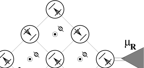
FIG. 10.: Schematic diagram of a $3\times 3$ array of quantum dots.

 

FIG. 11.: The partial width $\Gamma_{N}^{L}=\Gamma\sum_{\sigma}|\langle 0_{N}|d_{1\sigma}^{\dagger}|0_{N-1}\rangle|^{2}$ as a function of $N$ for the $3\times 3$ array of quantum dots with pure Hubbard interactions $U=10t$. The widths are plotted normalized by the partial width $\Gamma_{4}^{L}$ in (a) and $\Gamma_{5}^{L}$ in (b). The $x$ coordinate of the $N$th peak is given by $E_{N}^{0}-E_{N-1}^{0}$. Each peak is labeled by $N$. The peak structure is discussed in the text.

 

FIG. 12.: Conductance vs. chemical potential $\mu$ through the $3\times 3$ array of quantum dots. The same parameters used as in Fig. 6. The peak structure is discussed in the text.

REFERENCES

- [1] A. Yacoby, M. Heiblum, D. Mahalu, nad H. Shtrikman, Phys. Rev. Lett. 74, 4047 (1995); A. Yacoby, R. Schuster, and M. Heiblum, Phys. Rev. B 53, 9583 (1996); R. Schuster et al., Nature (London) 385, 417 (1997).
- [2] A. Levy Yeyati and M. Büttiker, Phys. Rev. B 52, 14360 (1995); G. Hackenbroich and H. Weidenmuller, Phys. Rev. Lett. 76, 110 (1996); C. Bruder, R. Fazio, and H. Schoeller, ibid. 76, 114 (1996).
- [3] M. Büttiker and C. A. Stafford, Phys. Rev. Lett. 76, 495 (1996); in Correlated Fermions and Transport in Mesoscopic Systems, T. Martin, G. Montambaux, and J. Tran Thanh Van eds., p. 491 (Editions Frontières, Gif-sur-Yvette, 1996).
- [4] A. Lorke, J. P. Kotthaus, and K. Ploog, Phys. Rev. Lett. 64, 2559 (1990); L. P. Kouwenhoven et al., ibid. 65, 361 (1990);
- [5] M. Tewordt et al., Phys. Rev. B 49, 8071 (1994); M. Kemerink and L. W. Molenkamp, Appl. Phys. Lett. 65, 1012 (1994).
- [6] N. C. van der Vaart et al., Phys. Rev. Lett. 74, 4702 (1995); D. Dixon et al., Phys. Rev. B 53, 12625 (1996).
- [7] F. R. Waugh et al., Phys. Rev. Lett. 75, 705 (1995); F. R. Waugh, M. J. Berry, and A. C. Gossard, Phys. Rev. B 53, 1413 (1996).
- [8] F. Hofmann et al., Phys. Rev. B 51, 13872 (1995).
- [9] R. H. Blick et al., Phys. Rev. B 53, 7899 (1996).
- [10] C. Livermore et al., Science 274, 1332 (1996); C. H. Crouch et al., Appl. Phys. Lett. 71, 817 (1997).
- [11] D. V. Averin, A. N. Korotkov, and K. K. Likharev, Phys. Rev. B 44, 6199 (1991); C. W. J. Beenakker, ibid. 44, 1646 (1991); Y. Meir, N. S. Wingreen, and P. A. Lee, Phys. Rev. Lett. 66, 3048 (1991).
- [12] C. A. Stafford and S. Das Sarma, Phys. Rev. Lett. 72, 3590 (1994).
- [13] G. Klimeck, G. Chen, and S. Datta, Phys. Rev. B 50, 2316 (1994); G. Chen et al., ibid. 8035 (1994).
- [14] K. A. Matveev, L. I. Glazman, and H. U. Baranger, Phys. Rev. B 53, 1034 (1996); J. M. Golden and B. I. Halperin, ibid. 53, 3893 (1996).
- [15] C. A. Stafford and S. Das Sarma, Phys. Lett. A 230, 73 (1997).
- [16] R. Kotlyar and S. Das Sarma, Phys. Rev. B 56, 13235 (1997).
- [17] P. W. Anderson, Phys. Rev. 115, 2 (1959).
- [18] C. A. Stafford, Phys. Rev. B 48, 8430 (1993).
- [19] H.-L. Engquist and P. W. Anderson, Phys. Rev. B 24, 1151 (1981).
- [20] M. Büttiker, IBM J. Res. Dev. 32, 63 (1988).
- [21] D. V. Averin and K. K. Likharev, in Mesoscopic Phenomena in Solids, edited by B. L. Altshuler, P. A. Lee, and R. Webb (Elsevier, Amsterdam, 1991); I. M. Ruzin et al., Phys. Rev. B 45, 13469 (1992); A. A. Middleton and N. S. Wingreen, Phys. Rev. Lett. 71, 3198 (1993).
- [22] M. Büttiker, H. Thomas, and A. Prêtre, Phys. Lett. A 180, 364 (1993).
- [23] C. A. Stafford, Phys. Rev. Lett. 77, 2770 (1996).
- [24] Holger Frahm and V. E. Korepin, Phys. Rev. B 43, 5653 (1991); J. M. P. Carmelo, P. Horsch, and A. A. Ovchinnikov, ibid. 45, 7899 (1992).
- [25] O. Klein et al., Phys. Rev. Lett. 74, 785 (1995).
- [26] Y. Meir and N. S. Wingreen, Phys. Rev. Lett. 68, 2512 (1992).
- [27] M. Büttiker, Phys. Rev. Lett. 57, 1761 (1986).
- [28] E. B. Foxman et al., Phys. Rev. B 47, 10020 (1993).
- [29] A. T. Johnson et al., Phys. Rev. Lett. 69, 1592 (1992); T. Heinzel et al., Europhys. Lett. 26, 689 (1994).
- [30] D. C. Ralph, C. T. Black, and M. Tinkham, Phys. Rev. Lett. 74, 3241 (1995); C. T. Black, D. C. Ralph, and M. Tinkham, ibid., 76, 688 (1996).
- [31] Eq. (9) is applicable to tunneling through superconducting systems in which the charging energy exceeds the superconducting gap, so that Andreev reflection is energetically prohibited.
- [32] S. Hershfield, J. H. Davies, and J. W. Wilkins, Phys. Rev. B 46, 7046 (1992); A. Levy Yeyati, A. Martín-Rodero, and F. Flores, Phys. Rev. Lett. 71, 2991 (1993); N. S. Wingreen and Y. Meir, ibid., 49, 11040 (1994), and refs. therein.
- [33] C. Bruder, R. Fazio, and H. Schoeller, Phys. Rev. Lett. 76, 114 (1996).
- [34] A. Schiller and S. Hershfield, Phys. Rev. B 51, 12896 (1995).
- [35] P. W. Anderson, Phys. Rev. Lett. 18, 1049 (1967).
- [36] J. M. Kinaret et al., Phys. Rev. B 46, 4681 (1992).
- [37] R. Dashen, S.-K. Ma, and H. J. Bernstein, Phys. Rev. 187, 345 (1969).
- [38] E. Akkermans, A. Auerbach, J. E. Avron, and B. Shapiro, Phys. Rev. Lett. 66, 76 (1991).
- [39] A. J. Leggett, in Granular Nanoelectronics, edited by D. K. Ferry et al. (Plenum, New York, 1991), p. 297; D. Loss, Phys. Rev. Lett. 69, 343 (1992).
- [40] The parallel quantum dot geometry of Hofmann et al. [8] should exhibit a similar magnetoresistance effect in the thermally broadened resonance regime.
- [41] E. Dagotto, Rev. Mod. Phys. 66, 763 (1994).
- [42] Note that and commute with the Hamiltonian, Eqs. (1) and (4), although the total spin does not, due to the spin-dependent disorder, Eq. (2).
- [43] C. A. Stafford and A. J. Millis, Phys. Rev. B 48, 1409 (1993).
- [44] K. Flensberg, Phys. Rev. B 48, 11156 (1993); K. A. Matveev, ibid. 51, 1743 (1995); G. Falci, G. Schön, and G. T. Zimanyi, Physica B 203, 409 (1994).
- [45] An analogous effect in CDW systems is discussed by T. Giamarchi and B. S. Shastry, Phys. Rev. B 51, 10915 (1995).
- [46] In contrast, for coupled GaAs quantum dots smaller than about 100nm in diameter, the breakdown of CCB is expected to occur [12] for , when the transmission through the interdot barriers is less than unity.
- [47] R. Kotlyar and S. Das Sarma, Phys. Rev. B 55, R10 205 (1997); R. Kotlyar, C. A. Stafford, and S. Das Sarma, unpublished (1997).
- [48] D. Weinmann, W. Hausler, and B. Kramer, Phys. Rev. Lett. 74, 984 (1995).