Noise properties and ac conductance of mesoscopic diffusive conductors with screening

Abstract

A theory of non-equilibrium (“shot”) noise and high frequency conductance in diffusive mesoscopic conductors with screening is presented. Detailed results are obtained for two simple geometries, for both large and short electron-electron scattering length $l_{ee}$, at frequencies of the order of the inverse Thouless time $1/\tau_{T}$. The conductance and the noise are found to exhibit significant frequency dependence. For $L\ll l_{ee}$, the high-frequency ($\omega\tau_{T}\gg 1$) shot noise spectral density $S_{I}(\omega)$ approaches a finite value between $2eI/3$ and $2eI$, depending on the screening properties of the system, with temperature corrections to $S_{I}(\omega)$ being linear in $T$. However, when $L\gg l_{ee}$, $S_{I}(\omega)$ grows as $\omega^{1/4}$ (at $T=0$), is not upper-bound by $2eI$, and has a temperature-dependent component quadratic in $T$. As a result, measurements of $S_{I}(\omega,T)$ can be utilized as a probe of the strength of electron-electron scattering.

I introduction

Significant attention has recently been focused on the dynamic electronic properties of mesoscopic systems. These properties include the ac conductance which gives the mean current response to applied ac voltage, and the noise, i.e., the deviations of the current from its average value. Due to the fluctuation-dissipation theorem, equilibrium Johnson-Nyquist noise, as measured in the external leads, does not convey any additional information to that obtained from the ac conductance. This is not the case for non-equilibrium (’shot’) noise. Here, the current fluctuations are dependent upon the non-equilibrium distribution function, as well as on electron-electron correlations. Moreover, the shot noise may be interpreted as an indication that the transport mechanism through the structure involves discrete transfer of charge, as opposed to the continuous charge transfer that takes place in macroscopic conductors.[1]

Earlier, shot noise in diffusive conductors was calculated in the zero-frequency limit,[2, 3, 4, 5] with the conclusion that the low frequency spectral density equals 1/3 of the classical Schottky value $2eI$, where $I$ is the average (dc) current in the system. This result was obtained in two very different theoretical frameworks, namely in a quantum mechanical transmission approach[2] which is generally based on the quantum coherence of the different electron states, and in a semi-classical approach,[3] in which quantum coherence is neglected, and the only effects on the noise are due to the single-particle non-equilibrium distribution function of the electrons. We believe that this surprising agreement between the two theories was adequately explained[6] by showing that the main ingredient in the transmission approach, the probability distribution of transmission coefficients, is not affected by quantum interference in diffusive conductors, thus establishing the validity of the semi-classical method.[7] The 1/3 suppression result is strictly valid only in a non-interacting electron picture. The electron-electron interaction slightly increases the zero-frequency noise value, which reaches $(\sqrt{3}/2)eI$ in the limit when the electrons are locally thermalized.[8, 9]

One of the most important characteristics of classical shot noise is that it is white up to very high frequencies. In ballistic structures the noise is reduced only at frequencies of the order of the inverse time of flight of the electron across the device.[10] In diffusive conductors, there are at least three a priori candidates to the analog of this time constant: the elastic scattering time $\tau$, the (much larger) “Thouless” time $\tau_{T}$ of electron diffusion through the sample, and the Maxwell relaxation time $(4\pi\sigma)^{-1}$. In addition, quantum effects also may be manifested by a frequency-dependent noise spectrum, increasing the noise at $\omega>~{}eV/\hbar$, where $V$ is the applied voltage.[11] Recently we have shown[12] that even at high voltage, $eV\gg\hbar/\tau_{T}$, where quantum effects are negligible, the shot noise in diffusive structures may exhibit considerable frequency dependence at frequencies as low as $1/\tau_{T}$.[13] In that work, however, only the zero-temperature case was considered and the ac conductance and effects of electron-electron interaction were not explored.

The issue of high-frequency noise cannot be separated from that of the ac conductance at the same frequency. Previous works studied the ac conductance in diffusive structures with ring[14, 15, 16] or linear[17, 18, 19] geometries. In the first case, non-interacting electrons were considered, and the frequency dependence of the ac conductance was found to be similar to the Drude dependence,[15] i.e., appreciable only at $\omega\sim 1/\tau$. However, usual conductors (with electrodes) cannot be considered separately from their electrodynamic environment. For such conductors general expressions for the conductivity were obtained to linear order in the frequency.[17, 18, 19] Under the assumption of absolute local electro-neutrality, it was found that this linear correction (the “emittance”) vanishes and the conductance is again independent of the frequency up to $\omega\sim 1/\tau$.[19] Here we are interested in the case where the conductor’s length $L$ or its thickness $t$ are comparable to the screening length $\lambda$, so local charge neutrality may no longer be retained. While we confirm the previous results[19] for $L,t\gg\lambda$, we show that observable deviations from them may appear already at $L/\lambda\sim 10$ or $t/\lambda\sim 10$.

A vast amount of research has been dedicated to the effects of weak localization on the dc conductance of mesoscopic diffusive conductors.[20] Its effect on the ac conductance[21] and the high temperature noise ($T>eV$)[22] lead to corrections to these quantities which are of the order of the quantum unit of conductance $e^{2}/h$ (times some characteristic energy in the case of noise). These corrections will be neglected in this work, since we will consider the case of conductance much higher than $e^{2}/h$, so that deviations of the high-frequency conductance and the noise from their zero-frequency values are much larger than the weak localization corrections.

In the present work the noise properties and the ac conductance of diffusive conductors much shorter than the electron-phonon mean free path are calculated at frequencies comparable $1/\tau_{T}$ or $4\pi\sigma$, with account of screening. Throughout the work we assume that the electrons form a degenerate gas with Fermi wavelength $\lambda_{F}$ much smaller than the elastic mean free path $l$, while $l\ll L,\lambda$. This allows us to use the Boltzmann-Langevin approach introduced by Kogan and Shulman[23] (see also Ref. [24]), and study both the ac conductance and the noise in a unified way. In section II we analyze the Boltzmann-Langevin equation in a non-uniform structure, obtain the boundary conditions for the distribution function at the conductor-electrode interface, and derive a “drift-diffusion-Langevin” equation for the current. In section III we apply this equation to two specific models of diffusive conductors (a “sandwich” and a conductor over a ground plane). In section IV the kernels, which describe the response of the system to external voltage, and to the random Langevin sources, are found. Using these response functions we calculate the conductance and thermal noise (section V), and the non-equilibrium shot noise (section VI). Section VII presents discussion of the results and conclusions.

II Boltzmann-Langevin-Poisson theory

In order to describe both the conductor and electrodes, we need self-consistent equations for the current in a system which may be substantially non-uniform on a scale $\Delta r\gg l$. In the diffusion approximation the electron distribution function can be written as

$$f=f(\varepsilon,\cos\theta,{\bf r},t)=f_{s}(\varepsilon,{\bf r},t)+f_{a}(\varepsilon,{\bf r},t)\cos\theta,$$ (1)

where $|f_{a}|\sim l/L\ll 1$ and $\varepsilon$ is the total electron energy,

$$\varepsilon=\varepsilon_{\bf k}+\varepsilon_{c}({\bf r})-e\Phi({\bf r},t)\equiv\varepsilon_{\bf k}+U({\bf r},t).$$ (2)

Here $\varepsilon_{\bf k}$ is the kinetic energy of an electron with momentum ${\bf k}$ while $\varepsilon_{c}({\bf r})$ is the equilibrium local conduction band edge, which includes possible band-bending due to mismatch in the local Fermi energies in the non-uniform conductor, and hence describes the equilibrium (“built-in”) electric field ${\bf E}_{0}=-\nabla\varepsilon_{c}/e$. $\theta$ is the angle between ${\bf k}$ and the direction of the current, and $\Phi({\bf r},t)$ is the time-dependent electric potential, so that $U({\bf r},t)$ is the total instantaneous potential energy of the electrons. In the above variables, the velocity of the particle is both position- and time-dependent, $v=v(\varepsilon,{\bf r},t)$, and the Boltzmann equation within the usual relaxation-time approximation looks like

$$\frac{\partial f}{\partial t}+\frac{\partial f}{\partial\varepsilon}\frac{\partial U}{\partial t}-\frac{\partial f}{\partial\cos\theta}\frac{\partial\cos\theta}{\partial{\bf k}}\cdot\nabla U$$ (3)

$$+\nabla f\cdot{\bf v}+\frac{f_{a}\cos\theta}{\tau} = 0$$ (4)

where $\tau=\tau({\bf r})$ is the local elastic relaxation time. Note that in the diffusion approximation the term proportional to $\nabla U$ is usually neglected, since it is of the order of $f_{a}^{2}$. However, in our case this term may be linear in $f_{a}$, because $\nabla U$ has the component $\nabla\varepsilon_{c}$ even in the absence of current.

As usual,[25] we proceed by separating Eq. (3) into its symmetric and antisymmetric parts [see Eq. (1)] and in the first order in $f_{a}$ we get

$$\frac{\partial f_{s}}{\partial t}+\frac{\partial f_{s}}{\partial\varepsilon}\frac{\partial U}{\partial t}-f_{a}\frac{\partial\cos\theta}{\partial{\bf k}}\cdot\nabla U + \nabla f_{a}\cdot{\bf v}\cos\theta=0,$$ (6)

$$\left(\frac{\partial}{\partial t}+\frac{1}{\tau}\right)f_{a}\cos\theta + \nabla f_{s}\cdot{\bf v}=0.$$ (7)

In this work we are interested only in the case of frequencies much smaller than $1/\tau$. In this case Eqs. (II) may be combined to give

$$\frac{\partial f_{s}}{\partial t}+\frac{\partial f_{s}}{\partial\varepsilon}\frac{\partial U}{\partial t}+\nabla f_{s}\cdot\frac{{\bf v}\tau}{\cos\theta}\frac{\partial\cos\theta}{\partial{\bf k}}\cdot\nabla U$$ (8)

$$-\nabla(\nabla f_{s}\cdot{\bf v}\tau)\cdot{\bf v} = 0.$$ (9)

Integration of this equation over the directions of ${\bf k}$ gives

$$\frac{\varepsilon_{\bf k}l}{D}\frac{\partial f_{s}}{\partial t}-\nabla\cdot\left[\varepsilon_{\bf k}l\nabla f_{s}\right]-\frac{3}{2}l\nabla_{\perp}f_{s}\cdot\nabla_{\perp}U=0$$ (10)

with $D=D({\bf r})=l({\bf r})v_{F}({\bf r})/3$ and $l=l({\bf r})=\tau({\bf r})v_{F}({\bf r})$, $v_{F}$ being the Fermi velocity. $\nabla_{\perp}$ denotes differentiation in the plane perpendicular to the current direction $x$. Eq. (10) is a generalization of the regular diffusion equation for the distribution function in the case when the potential or the mean free path change substantially in space.

The random nature of the scattering in the conductor may be described[23, 24] by a stochastic source term $J^{s}({\bf r},{\bf k},t)$, with zero average, added to the right hand side of Eq. (3). Its correlation function was found by Kogan and Shul’man[23] assuming Poisson statistics of the scattering events, and taking into account the Fermi correlations of the electrons. For the case of strong isotropic impurity scattering ($l\ll L$) the result reads

$$\left\langle J_{a}^{s}\right. \left.({\bf r},\varepsilon,t)J_{a}^{s}({\bf r}^{\prime},\varepsilon^{\prime},t^{\prime})\right\rangle=$$ (12)

$$\frac{6\delta({\bf r}-{\bf r}^{\prime})\delta(\varepsilon-\varepsilon^{\prime})\delta(t-t^{\prime})}{\tau({\bf r}){\cal N}({\bf r})}\bar{f}_{s}(\varepsilon,{\bf r})\left[1-\bar{f}_{s}(\varepsilon,{\bf r})\right],$$

where $J_{a}^{s}$ is the antisymmetric component of $J^{s}$, ${\cal N}({\bf r})$ is the local density of states at the Fermi level (excluding the spin degeneracy), and $\bar{f}$ the ensemble average of the distribution function.

Equations for the current can be obtained by including the source term $J^{s}$ in equations (II), and then integrating them over the electrons’ momenta. It is convenient at this stage to change variables in Eqs. (II) from $\varepsilon$ to $\varepsilon_{\bf k}$ by using Eq. (2). Integrating Eq. (6) over ${\bf k}$, we get the continuity equation

$$\frac{\partial}{\partial t}\rho({\bf r},t)+\nabla\cdot{\bf j}({\bf r},t)=0$$ (13)

with ${\bf j}({\bf r},t)$ the current density, and $\rho({\bf r},t)$ the excess electron density, i.e., the total charge density minus its equilibrium value $\rho_{0}({\bf r})$ (which includes the possible charge transfer when two materials have been brought into contact). The Langevin term integrates out from this equation, as expected for particle-conserving scattering processes.

If, before integration over ${\bf k}$, we multiply Eq. (7) (including the Langevin term) by ${\bf v}$, it yields

$${\bf j}({\bf r},t) = -D({\bf r})\nabla\left[\rho_{0}({\bf r})+\rho({\bf r},t)\right]$$ (15)

$$+\left[\sigma({\bf r})+\delta\sigma({\bf r},t)\right]\left[{\bf E}_{0}({\bf r})+{\bf E}({\bf r},t)\right]+{\bf j}^{s}({\bf r},t)$$

with $\sigma({\bf r})=e\tau({\bf r})\rho_{0}({\bf r})/m({\bf r})$ and $\delta\sigma({\bf r},t)=e\tau({\bf r})\rho({\bf r},t)/m({\bf r})$. Here $m({\bf r})$ is the local effective mass (for simplicity, the parabolic and isotropic dispersion relation was assumed), and

$${\bf j}^{s}({\bf r},t)=e\tau({\bf r})\sum_{{\bf k}}{\bf v}_{{\bf k}}{J}^{s}({\bf r},{\bf k},t).$$ (16)

At equilibrium, and in the absence of external fluctuation sources, the current ${\bf j}({\bf r},t)$ should vanish. Thus, the built-in electric field satisfies the equation

$$-D({\bf r})\nabla\rho_{0}({\bf r})+\sigma({\bf r}){\bf E}_{0}({\bf r})=0$$ (17)

which may be interpreted as the constancy of the electro-chemical potential at $V=0$ and $j^{s}=0$.

The terms proportional to $\delta\sigma({\bf r},t)$ in Eq. (15) are negligible if

$$e\left|\Phi_{0}({\bf r})+\Phi({\bf r},t)\right|\ll\varepsilon_{F}-\varepsilon_{c}({\bf r}),$$ (18)

(where $\varepsilon_{F}$ is the equilibrium Fermi energy [Fig. 1(a)]), i.e., if the band bending and the external potential are small compared to the local Fermi energy. Under the condition (18), equation (15), together with the constraint (17), yield the ’drift-diffusion-Langevin’ equation

$${\bf j}({\bf r},t)=\sigma({\bf r}){\bf E}({\bf r},t)-D({\bf r}){\bf\nabla}\rho({\bf r},t)+{\bf j}^{s}({\bf r},t)$$ (19)

where the variables include both the deterministic and stochastic parts.

The correlation function of the current sources ${\bf j}^{s}$ in any direction $\alpha$ follows from equations (12) and (16):

$$\left\langle{j}_{\alpha}^{s}({\bf r},t){j}_{\alpha}^{s}({\bf r}^{\prime},t^{\prime})\right\rangle=\delta({\bf r}-{\bf r}^{\prime})\delta(t-t^{\prime}){\cal S}({\bf r})$$ (20)

with the correlator

$${\cal S}({\bf r})=\frac{2}{3}e^{2}\tau({\bf r}){\cal N}({\bf r})v_{F}^{2}({\bf r})\int_{0}^{\infty}d\varepsilon\,\bar{f}_{s}(\varepsilon,{\bf r})\left[1-\bar{f}_{s}(\varepsilon,{\bf r})\right].$$ (21)

Now let us consider a system in which a homogeneous conductor connects two homogeneous electrodes with interfaces at $\pm L/2$, with the only source of inhomogeneity being the band bending due to charge transfer between the materials [Fig. 1(a)]. Let the interfaces be normal to the $x$ axis and much sharper than the screening lengths $\lambda,\lambda_{e}$ in the conductor and the electrodes, respectively. We define the interface regions to be the regions of width $2\delta$ around $\pm L/2$, with $l\ll\delta\ll\lambda,\lambda_{e},L$. A major assumption of this work is that the voltage in the system drops entirely in the bulk of the conductor, i.e., the resistances of the electrodes and the electrode-conductor interfaces are small compared to that of the conductor. This is the natural situation when the electrodes are of high conductivity and when the interfaces are smooth on the scale of $\lambda_{F}$, so no reflections of electrons occur at the interfaces.

Let us consider, for example, the interface at $L/2$ and define $f_{s}^{c}=f_{s}(L/2-\delta)$ and $f_{s}^{e}=f_{s}(L/2+\delta)$. Since the voltage drop in the electrode is negligible, $f_{s}^{e}$ is just the equilibrium Fermi-Dirac distribution

$$f_{s}^{e}=f_{0}(\varepsilon+eV/2)=\frac{1}{1+\exp\left(\frac{\varepsilon+eV/2-\mu}{T}\right)},$$ (22)

where the chemical potential $\mu$ is defined as the average of the chemical potentials in the two electrodes. Moreover, the fact that there is no voltage drop across the interface region implies that $f_{s}^{c}$ is also given by Eq. (22), $f_{s}^{c}=f_{s}^{e}$. Integrating this equation over the electron’s momenta and using the relation ${\cal N}({\bf r})=1/4\pi e^{2}\lambda^{2}({\bf r})$ leads to the first boundary condition at the electrode-conductor interface,

$$\lambda^{2}\rho^{c}=\lambda_{e}^{2}\rho^{e}$$ (23)

with $\rho^{c}\equiv\rho(L/2-\delta)$ and $\rho^{e}\equiv\rho(L/2+\delta)$.

The second boundary condition is the continuity of the current across the interface,

$$j_{\omega x}^{c}=j_{\omega x}^{e}$$ (24)

with $j_{\omega x}^{c}$, $j_{\omega x}^{e}$ the Fourier components of the transverse current density at $L/2-\delta$, $L/2+\delta$, respectively.[26]

If complemented with the Poisson equation

$$\nabla\cdot{\bf E}({\bf r},t)=\frac{4\pi}{\epsilon({\bf r})}\rho({\bf r},t),$$ (25)

where $\epsilon({\bf r})$ is the dielectric constant, equations (13) and (19 – 25) form a closed system which is the basis for our calculations.

III Models

A The sandwich model

We study two analytically solvable models which differ in their assumed sample geometry, and hence in electrostatics.[12] In our first, “sandwich” model, which is schematically shown in Fig. 1(b), a short conductor of length $L\ll t$ is sandwiched between two wide electrodes ($t$ is the smallest transverse dimension of the conductor). Defining the quantities $\Phi_{\omega}(x)$, $q_{\omega}(x)$, $E_{\omega}(x)$, $I_{\omega}(x)$ and $I_{\omega}^{s}(x)$ as integrals over the sample’s cross-section of the temporal Fourier components of $\Phi({\bf r},t)$, $\rho({\bf r},t)$, $E_{x}({\bf r},t)$, $J_{x}({\bf r},t)$, and $j^{s}_{x}({\bf r},t)$, respectively, we get from equations (13, 19, 25)

$$-i\omega q_{\omega}(x)+\frac{dI_{\omega}(x)}{dx}=0,$$ (26)

$$I_{\omega}(x)=\sigma(x)E_{\omega}(x)-D(x)\frac{dq(x)}{dx}+I_{\omega}^{s}(x),$$ (27)

$$\frac{dE_{\omega}(x)}{dx}=\frac{4\pi}{\varepsilon(x)}q_{\omega}(x).$$ (28)

[Deriving Eq. (28), we have neglected the transverse derivatives of ${\bf E}({\bf r},t)$, since, by Gauss’ theorem, they are proportional to the circumference of the cross-section of the sample, while the derivative in the $x$-direction is proportional to the cross-section area.]

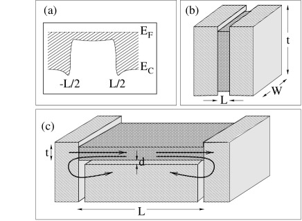
FIG. 1.: Schematic description of the geometries studied. (a) The conduction band-edge profile in both models. (b) The sandwich model. (c) The ground-plane model.

Integration of equations (26) and (28) provides a simple relation between the current and the electric field,

$$I_{\omega}(x)=\frac{i\omega\varepsilon(x)}{4\pi}E_{\omega}(x)+I_{\omega}^{e}.$$ (29)

The integration constant $I_{\omega}^{e}$ has the physical sense of the current induced deep inside the electrodes (where $E_{\omega}=0$). It can be found from the condition that the current fluctuations do not affect the voltage $V_{\omega}$ applied to the structure:

$$\int_{-\infty}^{\infty}dx\,\frac{4\pi}{i\omega\epsilon(x)}\left[I_{\omega}^{e}-I_{\omega}(x)\right]=V_{\omega}.$$ (30)

Inserting equations (26) and (29) in Eq. (27) we get the basic equation of this model,

$$\frac{d^{2}I_{\omega}(x)}{dx^{2}}-\kappa^{2}(x,\omega)I_{\omega}(x)=\frac{i\omega}{D(x)}I_{\omega}^{s}(x)-\frac{1}{\lambda^{2}(x)}I_{\omega}^{e},$$ (31)

with

$$\kappa^{2}(x,\omega)=\frac{1}{\lambda^{2}(x)}-\frac{i\omega}{D(x)}.$$ (32)

This equation is valid for both the conductor itself and the electrodes.

B The ground-plane model

In the second (“ground plane”) model we consider a long and thin conductor close and parallel to a well-conducting ground plane, $L\gg t,d$ where $t$ is the thickness of the conductor, and $d$ its distance from the ground-plane – see Fig. 1(c). The width of the conductor $W$ (i.e., its second dimension, parallel to the ground plane) can be arbitrary. As we will show below, this geometry is more promising for experimental observation of some of the effects studied in this work.

In the same way as for the previous model, equations (13) and (19) can be replaced with their 1D versions, i.e., equations (26) and (27), respectively. The Poisson equation, however, leads to a different one-dimensional equation since in this model the gradient of the field in the $x$-direction is much smaller than the transverse gradients. In this case, the linearity of the Poisson equation leads to a linear dependence of the potential on the local charge, both integrated over the conductor’s cross-section:

$$\Phi_{\omega}(x)=\frac{Aq_{\omega}(x)}{C_{0}},$$ (33)

where $A$ is the cross-sectional area and $C_{0}$ is the specific capacitance (per unit length).

For a homogeneous cylindrical conductor of radius $R=t/2$ and distance $h=t/2+d$ between its center and the ground plane $C_{0}$ assumes the following limiting values: if the conductor is thick ($t\gg\lambda$)[27]

$$C_{0}=\frac{\epsilon_{m}}{2\cosh^{-1}\left(h/R\right)}\,\,\,\,\,\,\,\,(R\gg\lambda),$$ (34)

with $\epsilon_{m}$ the dielectric constant of the medium between the conductor and the ground plane. In the opposite limit, the cylinder is uniformly charged. Taking for simplicity $\epsilon=\epsilon_{m}$, one finds

$$C_{0} = \frac{2\epsilon}{1+4\ln(h/R)+4I(h/R)}$$ (35)

$$\simeq \frac{2\epsilon}{1+4\ln\left(2h/R\right)},{\,\,\,\,\,\,\,\,}{\,\,\,\,\,\,\,\,}{\,\,\,\,\,\,\,\,}(R\ll\lambda),$$ (36)

with

$$I(b)\equiv\int_{0}^{1}dx\,\ln\left(1+\sqrt{1-\frac{x}{4b^{2}}}\right).$$ (37)

The dependences of $C_{0}$ on the ratio $R/h$ are shown in Fig. 2.

FIG. 2.: The dependence of $C_{0}$ on $R/h=t/(t+2d)$ for an homogeneous cylindrical conductor close to a ground plane.

If the conductor is a uniform strip of width $W\gg d,t$, then

$$C_{0} = \frac{W}{4\pi d},{\,\,\,\,\,\,\,\,}(t\gg\lambda),$$ (39)

$$C_{0} = \frac{W}{4\pi(d+t/3)},{\,\,\,\,\,\,\,\,}(t\ll\lambda).$$ (40)

In the quantum limit, with only the first quantum level populated, $C_{0}$ may still be presented with Eq. (40), though the thickness $t$ must be replaced by an effective thickness $t_{\rm eff}$. For a square well potential with infinite barriers the effective thickness is

$$t_{\rm eff}=t\left(1+\frac{3}{4\pi^{2}}\right)\simeq 1.07t.$$ (41)

Combining Eq. (27) with Eq. (33) provides a diffusion-like relation between the current and the linear charge density,

$$I_{\omega}(x)=-D^{\prime}\frac{dq_{\omega}(x)}{dx}+I^{s}(x),$$ (42)

with

$$D^{\prime}=D+\frac{\sigma A}{C_{0}}.$$ (43)

With the help of Eq. (26) we once again get a simple equation for the current

$$\frac{d^{2}I_{\omega}(x)}{dx^{2}}-\bar{\kappa}^{2}(\omega)I_{\omega}(x)=-\bar{\kappa}^{2}(x,\omega)I_{\omega}^{s}(x),$$ (44)

with

$$\bar{\kappa}^{2}(\omega)=-\frac{i\omega}{D^{\prime}}.$$ (45)

Thus, as seen by comparing equations (31, 32) with equations (44, 45), static screening effectively vanishes in this model, and only dynamic screening is important.

We now analyze the conditions under which Eq. (33) is valid. Expanding Eq. (44) in spatial harmonics we see that harmonics with wavenumber $k_{x}\gg|\bar{\kappa}|=\sqrt{\omega/D^{\prime}}$ contribute negligibly to the current fluctuations $I_{\omega}$. Thus, at frequencies $\omega\lesssim{{\bar{\tau}}_{T}}^{-1}\equiv D^{\prime}/L^{2}\ll D^{\prime}/d^{2},D^{\prime}/t^{2}$, we can consider only the wavenumbers $k_{x}$ which are much smaller than $d^{-1}$, $t^{-1}$. For these harmonics, the transversal gradients of the electric field dominate in the Poisson equation, justifying Eq. (33) at that frequency range.

Equation (33) is not valid at distances comparable to $d$ from the interface with the electrodes. Eq. (44) should therefore be solved only inside the conductor, with boundary conditions at $\pm\frac{L^{\prime}}{2}=\pm(\frac{L}{2}-\delta)$, where $\delta$ is now some distance for which $d\ll\delta\ll L,1/|\bar{\kappa}|$. To find these boundary conditions we write down Eq. (27) (which is valid even near the interface) in the form

$$I_{\omega}(x)=-\sigma\frac{d}{dx}\left[\Phi_{\omega}(x)+4\pi\lambda^{2}\ q_{\omega}(x)\right].$$ (46)

[The sources $I^{s}(x)$ in the small interface region may be neglected.] The values of $q_{\omega}$ and $\Phi_{\omega}$ at the actual interfaces $x=\pm L/2$ are found from the boundary conditions Eqs. (23, 24). First note that while $q_{\omega}$ can be arbitrarily large on the electrode side, $\lambda_{e}q_{\omega}$ should remain finite, since it is equal to the total interface charge in the electrode. In the case when the screening length in the electrodes $\lambda_{e}$ is much shorter than $\lambda$, Eq. (23) therefore gives (on the conductor side of the interface)

$$q_{\omega}\left(\pm\frac{L}{2}\right)=0.$$ (47)

Since the voltage drop in the electrode vanishes, the constraint of fixed voltage [i.e., the equivalent of Eq. (30)] in this model becomes

$$\Phi_{\omega}\left(\pm\frac{L}{2}\right)=\mp\frac{V_{\omega}A}{2}.$$ (48)

Integration of Eq. (46) from $\pm L/2$ to $\pm L^{\prime}/2$, and use of Eq. (33) at $\pm L^{\prime}/2$, now yields the required boundary conditions,

$$q_{\omega}\left(\pm\frac{L^{\prime}}{2}\right)=\mp\frac{V_{\omega}A\sigma}{2D^{\prime}}.$$ (49)

In this ground-plane model, finite charge densities in the conductor create image charges on the ground plane. Thus, at any finite frequency $\omega$ some parts of the interface currents are responsible for periodic re-charging of the ground plane [see Fig. 1(c)]. Therefore, the current $I_{\omega}^{e}$ measured in the electrodes at a distance far from conductor-electrode interface may be different from the current which flows through this interface (note also that the two interface currents are not necessarily equal). In an experimental scheme symmetric with respect to the conductor, the current $I_{\omega}^{e}$ flowing into the external circuit is the symmetric component of the two currents:

$$I_{\omega}^{e}=\frac{1}{2}\left[I_{\omega}\left(-\frac{L}{2}\right)+I_{\omega}\left(\frac{L}{2}\right)\right].$$ (50)

While the currents $I_{\omega}(\pm L/2)$ in this expression are the currents at the electrode side of the interfaces, due to Eq. (24) they are equal to $I_{\omega}(\pm L^{\prime}/2)$. Of course, if the leads connecting the sample to the measurement instrument have some mutual capacitance, the current in the instrument will be less than $I^{e}(\omega)$ given by Eq. (50), but this loss factor may be taken into account by the standard circuit theory methods.

IV The response functions

From now on we will consider the most natural case of well-conducting electrodes of size much larger than $\lambda_{e}$, and resistance negligible in comparison with the resistance $R=L/\sigma A$ of the conductor. We first show that the total noise produced in the electrodes is negligible compared to that originating in the conductor. For equilibrium noise, this is a direct consequence of the fluctuation-dissipation theorem. The same is true for shot noise, because of the fact that the electron distribution function in the electrodes is almost equilibrium. The electrode-conductor interface is also not an appreciable source of noise since, in the diffusion approximation studied here, the electron distribution at the conductor-side of the interface is the same equilibrium Fermi distribution as in the electrode. Moreover, even deviations from this approximation would result at the most in a few inelastic scattering events in the electrodes, leading to thermalization of hot electrons arriving from the conductor. As long as $l\ll L$, the number of those events per transfered electron is much smaller than the number of elastic events [$\sim(L/l)^{2}$] the electron experiences in the conductor, so the thermalization process at the interface can also be neglected as a source of noise.

In this situation, the solutions to equations (31) and (44) can thus be presented in the form

$$I_{\omega}(x)=Y(x;\omega)V_{\omega}+\frac{1}{L}\int_{-\frac{L}{2}}^{\frac{L}{2}}K(x,x^{\prime};\omega)I_{\omega}^{s}(x^{\prime})\,dx^{\prime}.$$ (51)

Eq. (51) shows that the current at frequency $\omega$ at any point $x$ is composed of two components. The first is the response to the applied voltage across the conductor, and the second is the response to the random Langevin current sources inside the conductor.

The response functions $Y(x;\omega)$ and $K(x,x^{\prime};\omega)$ are found by solving the equations for the current with $I_{\omega}^{s}(x)=0$ and $V_{\omega}=0$, respectively. They can be presented in a compact form by defining the following auxiliary functions, with $\eta=\kappa\lambda^{2}/\lambda_{e}$, $u=\kappa L/2$, ${\rm sinch}(u)=\sinh(u)/u$, $\Omega=\omega/4\pi\sigma$, and $\chi=|x|-L/2$:

$${\cal D}(\omega)=\frac{1}{\cosh(u)+\eta\sinh(u)},$$ (52)

$${\cal E}_{\pm}(x,\omega)=\left\{\begin{array}[]{ll}\frac{u}{1-i\Omega}\left[\sinh(u\pm\kappa x)+\eta\cosh(u\pm\kappa x)\right]&(|x|<\frac{L}{2}),\\ \frac{u}{1-i\Omega}\eta\exp(-\kappa_{e}\chi)&(|x|>\frac{L}{2}),\end{array}\right.$$ (53)

$${\cal F}(x,\omega)=\left\{\begin{array}[]{ll}\frac{1-i\Omega{\cal D}(\omega)\cosh(\kappa x)}{\left[1-i\Omega\right]\left[1-i\Omega{\cal D}(\omega){\rm sinch}(u)\right]}&(|x|<\frac{L}{2}),\\ \frac{1-i\Omega\left[1-\eta{\cal D}(\omega)\sinh(u)\exp(-\kappa_{e}\chi)\right]}{\left[1-i\Omega\right]\left[1-i\Omega{\cal D}(\omega){\rm sinch}(u)\right]}&(|x|>\frac{L}{2}),\end{array}\right.$$ (54)

$${\cal G}_{\pm}(x,\omega)=\frac{i\Omega{\cal E}_{\pm}(x,\omega)}{\sinh(u)+\eta\cosh(u)},$$ (55)

$${\cal H}_{\pm}(x,\omega)=i\Omega{\cal D}(\omega)\left[{\cal F}(x,\omega)+{\cal E}_{\pm}(x,\omega)\right].$$ (56)

For the sandwich model, the response functions are

$$K(x,x^{\prime};\omega) = {\cal F}(x,\omega)\pm{\cal G}_{\pm}(x,\omega)\sinh(\kappa x^{\prime})$$ (58)

$$-{\cal H}_{\pm}(x,\omega)\cosh(\kappa x^{\prime})$$

and

$$Y(x;\omega)=\frac{1-i\Omega}{R}{\cal F}(x,\omega),$$ (59)

where, in Eq. (58), the upper sign should be used for $x^{\prime}>x$ and the lower sign for $x^{\prime}<x$.

In the ground-plane model, the functions $K$ and $Y$ inside the conductor are found to be the same as for the sandwich model (but with $D\rightarrow D^{\prime}$) in the limit of vanishing conductivity of the conductor, i.e., in the formal limit $\eta^{2}\sim\Omega\rightarrow\infty$ (which also implies $\kappa=\bar{\kappa}$):

$$K(x,x^{\prime};\omega)=\cosh(\bar{u}\pm\bar{\kappa}x)\frac{\cosh(\bar{u}\mp\bar{\kappa}x^{\prime})}{{\rm sinch}(2\bar{u})}$$ (60)

with $\bar{u}=\bar{\kappa}L/2$ and with the upper sign used for $x^{\prime}>x$ and the lower for $x^{\prime}<x$. The response in the electrodes $K^{e}(x^{\prime};\omega)$ to a fluctuation at $x^{\prime}$ is obtained with the help of Eq. (50),

$$K^{e}(x^{\prime};\omega)=\frac{\cosh(\bar{\kappa}x^{\prime})}{{\rm sinch}(\bar{u})}.$$ (61)

The response to voltage $Y(x,\omega)$ in this model is identical to $K^{e}(x;\omega)/R$,

FIG. 3.: Position dependence of the real (solid lines) and imaginary (dashed lines) parts of the response functions for the sandwich model at high frequencies, and for two values of $L/\lambda$. Re$[Y(x;\omega)]$ is in units of $1/R$. Im$[Y(x;\omega)]$ is in units of $-\Omega/R$. $x^{\prime}=0.3$ here.

$$Y(x;\omega)=\frac{1}{R}\frac{\cosh(\bar{\kappa}x)}{{\rm sinch}(\bar{u})}.$$ (62)

At low frequencies, and in both models, the response functions tend to constant values:

$$K(x,x^{\prime};0)=1,\,\,\,\,\,\,\,\,Y(x;0)=\frac{1}{R}.$$ (63)

Fig. 3 shows the response functions for the sandwich model at intermediate and high frequencies. At $\omega{{\tau}_{T}}\gg 1$ the responses are exponentially close to the source, i.e., to $x^{\prime}$ in the case of $K(x,x^{\prime};\omega)$ and to $\pm L/2$ in the case of $Y(x;\omega)$. At any frequency and position, and for any value of $L/\lambda$,

$$\frac{1}{L}\int_{-\frac{L}{2}}^{\frac{L}{2}}K(x,x^{\prime};\omega)\,dx^{\prime}=1.$$ (64)

This general result is a manifestation of the constraint $V_{\omega}=0$, as can be seen by assuming a uniform current source in Eq. (51). Then, the only solution of the problem which maintains the constraint of fixed voltage is a uniform current everywhere, $I_{\omega}(x)=I_{\omega}^{s}$, leading immediately to Eq. (64).

The relation between the spectral density of the current noise $S_{I}(x,\omega)$ and the response function $K(x,x^{\prime};\omega)$ is made clear through the identity

$$S_{I}(x,\omega)\delta(\omega)=2\langle I_{\omega}(x)I_{\omega}^{*}(x)\rangle.$$ (65)

With Eq. (51), and using the condition of fixed voltage and the locality of the current correlator [Eq. (20)], this expression becomes

$$S_{I}(x,\omega)=\frac{2A}{L^{2}}\int_{-\frac{L}{2}}^{\frac{L}{2}}|K(x,x^{\prime};\omega)|^{2}{\cal S}(x^{\prime})\,dx^{\prime}.$$ (66)

The noise power deep inside the electrodes is given by

$$S_{I}(\omega)\equiv S_{I}(\infty,\omega).$$ (67)

The dynamic conductance is the response in the electrodes to external voltage,

$$Y(\omega)\equiv Y(\infty,\omega).$$ (68)

V Results: Conductance and equilibrium noise

A Sandwich model

For the sandwich model we have from equations (54), (59) and ( 68)

$$Y(\omega)=\frac{1-i\Omega}{R}\frac{1}{1-i\Omega{\cal D}(\omega){\rm sinch}(u)}.$$ (69)

If the screening length in the electrodes is very small compared to $L$ then $\eta u\gg 1$, and we get

$$Y(\omega)=\frac{1-i\Omega}{R}=R^{-1}-i\omega C,{\,\,\,\,\,\,\,\,}C=\frac{A}{4\pi L},$$ (70)

for any frequency $\omega$. Equation 70 allows a simple interpretation: $Y(\omega)$ is just the complex admittance of the conductance $R^{-1}$ coupled in parallel to the capacitor $C$ formed by the two electrodes.

            

FIG. 4.: The real and imaginary parts of the correction to the conductance of the sandwich model. The various curves are for different values of $L/\lambda$, and for $\lambda_{e}=\lambda$. (a) ${\cal D}(\omega){\rm sinch}(u)$. The low-frequency value of this quantity is equal to one plus the emittance of the system. (b) ${\cal F}^{e}(\omega)=Y(\omega)/[(1-i\Omega)/R]$.

However, already at $L/\lambda_{e}=10$ the correction

$${\cal F}^{e}(\omega)=\frac{1}{1-i\Omega{\cal D}(\omega){\rm sinch}(u)}$$ (71)

to this simple result is significant. Figure 4 shows the real and imaginary parts of this correction for different values of $L/\lambda$, for the case $\lambda=\lambda_{e}$ (for example, the conductor and the electrodes are made of the same material, but the electrodes have much fewer impurities). For $L/\lambda_{e}>1$ the correction term is insensitive to an increase of $\lambda$, so the appropriate curves of Fig. 4 also correspond to the case of a low-density conductor between metal electrodes. Fig. 4(a) shows the term ${\cal D}(\omega){\rm sinch}(u)$ which appears in the denominator of Eq. (69). The low-frequency value of this term is equal to $1-4\pi\sigma RE(0)$, with $\left.E(0)\equiv idY/d\omega\right|_{\omega=0}$ being the “emittance”. For a long conductor ($L/\lambda\gg 1$)

$$E(0)=\frac{A}{4\pi L}=\frac{1}{C}.$$ (72)

As in Eq. (70), the emittance in this case can be viewed as the sum of the intrinsic emittance of the conductor and that of the capacitor formed by the electrodes. Then, the total emittance (72) is entirely due to the parallel-plate capacitance, and the emittance of the “conductor itself” equals zero, in agreement with the result of Ref. [19]. However, as seen from Fig. 4(a), this result does not hold for a relatively short conductor, which means that the simple view of an additive emittance does not generally hold.

It is important to note that the calculations leading to Eq. (69) were not dependent on the distribution function of the electrons. Therefore, the correction to $Y(\omega)$ is due only to the screening properties of the system, and does not depend on thermalization or phase-breaking of the electrons. Equation (69) is thus also valid if the inelastic scattering length is smaller than $L$. Despite its mesoscopic nature [i.e., the fact that $Y(\omega)$ assumes its ordinary value Eq. (70) for large enough $L$], the correction discussed here should not be confused with other mesoscopic corrections to the conductivity of diffusive wires.[28]

B Ground-plane model

For the ground-plane model equations (50) and (62) lead to the following expression for the conductance of the system

$$Y(\omega)=\frac{1}{R}\left(\bar{\kappa}\frac{L}{2}\right){\rm cth}\left(\bar{\kappa}\frac{L}{2}\right).$$ (73)

This expression is identical to the conductance of a macroscopic wire of resistance $R$ coupled to the ground plane via capacitance per unit length of

$$C_{{\rm eff}}=\left(\frac{1}{C_{0}}+\frac{1}{C_{S}}\right)^{-1},$$ (74)

with

$$C_{S}=\frac{A}{4\pi\lambda^{2}}.$$ (75)

The boundary conditions for this model, Eq. (49), can also be rewritten in terms of $C_{\rm eff}$ as

$$q_{\omega}\left(\pm\frac{L^{\prime}}{2}\right)=\frac{V_{\omega}}{2}C_{\rm eff}.$$ (76)

Thus, the ground-plane model can be described by the equivalent circuit shown in Fig. 5. The capacitance $C_{S}$ is due to the fact that in thin enough wires the screening is not efficient, so the current is determined by the gradient of the full electrochemical potential $\varphi=\Phi+A\mu/e$, rather than by $\Phi=Aq_{\omega}/C_{0}$ alone. In other words, additional charging of the wire increases not only its electrostatic energy ($\propto C_{0}^{-1}$), but also its internal energy ($\propto C_{S}^{-1}$), because of the necessary rise in the Fermi level. In 2D conductors, Eq. (75) reduces to the well-known result[29] for the two-dimensional electron gas. There is also a very interesting analogy between Eq. (75) and the expression $L_{0}^{-1}=A/4\pi\lambda^{2}$[30] for the specific kinetic inductance of a superconductor (in this case $\lambda$ is London’s penetration depth).

   

FIG. 5.: Equivalent circuit for the geometry of the ground-plane model.

When $C_{s}\ll C_{0}$ the high frequency ($\omega{{\bar{\tau}}_{T}}\gg 1$) conductance is given by

$$Y(\omega)=\frac{1}{R}\frac{L}{2\sqrt{iD/\omega}}$$ (77)

which its absolute value is just the dc conductance of a conductor of the same conductivity $\sigma$, but with length equal to twice the diffusion distance in time $1/\omega$. Thus, carriers injected at each of the electrodes are diffusing in and out of the conductor, without reaching the opposite electrode, and without affecting it by electric fields (the suppression of the longitudinal electric fields is the only role of the ground plane in this limit).

C Equilibrium noise – both models

Equilibrium thermal noise is related to the conductance by the fluctuation-dissipation theorem (we assume $T\gg\hbar\omega$)

$$S_{I}^{{\rm eq}}(\omega)=4T{\rm Re}\left[Y(\omega)\right].$$ (78)

However, since $Y(x,\omega)$ gives the current response to the external voltage, the local noise $S_{I}^{{\rm eq}}(x,\omega)$ is not directly related to it, and must be calculated independently.

At zero voltage, the average distribution function in the conductor is the Fermi-Dirac distribution given by Eq. (22). Using this distribution in Eq. (21) gives

$${\cal S}=2\sigma T$$ (79)

for the correlator of the Langevin sources. The spectral density for the equilibrium noise is thus found from Eq. (66),

$$S_{I}^{{\rm eq}}(x,\omega)=\frac{4T}{RL}\int_{-\frac{L}{2}}^{\frac{L}{2}}|K(x,x^{\prime};\omega)|^{2}\,dx^{\prime};$$ (80)

this equation in fact expresses the fluctuation-dissipation theorem for both the local and external fluctuations.

At zero frequency Eq.(63) gives

$$S_{I}^{{\rm eq}}(x,0)=\frac{4T}{R},$$ (81)

as expected. At high frequencies ($\Omega,\omega{{\bar{\tau}}_{T}}\gg 1$), the equilibrium noise inside the conductor is given by

$$S_{I}^{\rm eq}(x,\omega)=\frac{2T}{R}\sqrt{\omega{{\bar{\tau}}_{T}}/2}\left[f(x)+f(-x)\right]{\,\,\,\,\,\,\,\,}(|x|<L/2)$$ (82)

with

$$f(x)=2e^{-\kappa_{1}L}|\cosh(u-\kappa x)|^{2}\left[e^{2\kappa_{1}x}-e^{-\kappa_{1}L}\right]$$ (83)

and with $\kappa_{1}={\rm Re}(\kappa)$, so $\kappa_{1}L=\sqrt{\omega{{\bar{\tau}}_{T}}/2}$. $f(x)=1/2$ throughout the conductor, except at a narrow layer of width $1/\kappa_{1}$ near the edges, where it approaches its limiting values $f(-L/2)=0$, $f(L/2)=2$. The position and frequency dependence of $S_{I}^{\rm eq}$ is shown in Fig. 6(a) for the case $L/\lambda=L/\lambda_{e}=10$. The general features here do not depend on screening.

FIG. 6.: Position and frequency dependence of the current noise intensity inside the conductor. (a) Equilibrium noise. (b) Shot noise. Here $L/\lambda=L/\lambda_{e}=10$, but the general features of this figure are not sensitive to the screening properties.

The method presented here for calculating the conductance does not depend on the form of the distribution function [other than the diffusion approximation, Eq. (1)]. Therefore the results apply also to the case when strong ($l_{ee}\ll L$, with $l_{ee}$ the electron-electron scattering length) electron-electron scattering is present in the conductor. The equilibrium noise is also not affected by the e-e processes since this scattering does not affect the equilibrium Fermi-Dirac distribution, which is the input in Eq. (21).

VI Results: Non-equilibrium noise

In this section we will present the results on non-equilibrium noise for the ground-plane model; these results are also applicable for the sandwich model in the regime $\lambda,\lambda_{e}\gg L$. In the opposite limit ($\lambda,\lambda_{e}\ll L$) the noise in the sandwich model is white and is equal to the zero-frequency noise in the ground-plane model.[12] In contrast to the case of equilibrium noise, the shot noise is very sensitive to the strength of electron-electron interaction in the conductor, so we analyze this noise in the two limits of weak and strong e-e scattering.

A Weak electron-electron scattering ($L\ll l_{ee}$)

When $L\ll l_{ee}$ the electron distribution function is found as a steady-state solution of Eq. (10). Under the condition (18) and for current perpendicular to the interfaces, it reads:[3]

$$\bar{f}_{s}(E,x) = \left(\frac{1}{2}+\frac{x}{L}\right)f_{0}\left(E+\frac{1}{2}eV\right)$$ (85)

$${\,\,\,\,\,\,\,\,}+\left(\frac{1}{2}-\frac{x}{L}\right)f_{0}\left(E-\frac{1}{2}eV\right).$$

Eq. (66) together with equations (21) and (22) now give a general expression for the non-equilibrium noise,

$$S_{I}(x,\omega)=\frac{2}{RL}\int_{-\frac{L}{2}}^{\frac{L}{2}}dx^{\prime}\,|K(x,x^{\prime};\omega)|^{2}\left[{\cal S}_{+}+{\cal S}_{-}\frac{4x^{\prime 2}}{L^{2}}\right]$$ (86)

with

$${\cal S}_{\pm}(T,V)=T\pm\frac{eV}{2}{\rm cth}\left(\frac{eV}{2T}\right).$$ (87)

Fig. 6(b) shows the spatial and frequency dependence of the shot noise for the case $L\gg\lambda,\lambda_{e}$ and $T\ll eV$. It is remarkable that inside the conductor the high-frequency noise is large even at zero temperature:

$$S_{I}(x,\omega)=\frac{eI}{2}\sqrt{\frac{\omega{{\bar{\tau}}_{T}}}{2}}\left(1-\frac{4x^{2}}{L^{2}}\right),{\,\,\,\,\,\,\,\,}(\omega{{\bar{\tau}}_{T}}\gg 1).$$ (88)

This rise is due to the highly non-equilibrium distribution of carriers, Eq. (85). Specifically, at any frequency $\omega$ the current fluctuations at position $x$ are due only to electrons at distances $\sim\sqrt{\bar{D}/\omega}$ from $x$. The smaller this range, the smaller is the smoothing of the singularity in the energy distribution of the electrons in the range, and the larger the noise.

The noise in the external electrodes is found by using the external response function $K^{e}(x^{\prime};\omega)$ in Eq. (86). Whenever $K^{e}(x^{\prime};\omega)=1$, i.e., at low frequencies, or when $\lambda,\lambda_{e}\ll L$ in the sandwich model, Eq. (86) reduces to

$$S_{I}(\omega)=\frac{4}{R}\left[\frac{2}{3}T+\frac{1}{6}eV{\rm cth}\left(\frac{eV}{2T}\right)\right]$$ (89)

as was found by Nagaev.[3] However, in the general case, the noise in the electrodes exhibits strong frequency dependence on a frequency scale of the order of the inverse effective Thouless time $1/{\bar{\tau}}_{T}$, which is also affected by the screening lengths $\lambda$, $\lambda_{e}$.[12] Figure 7(a,b) shows the dependence of the noise on frequency and temperature in the ground-plane model. At $\omega{{\bar{\tau}}_{T}}\gg 1$

$$S_{I}(\omega)=\frac{2T}{R}\left(\sqrt{\omega{{\bar{\tau}}_{T}}/2}-1\right)+eI{\rm cth}\left(\frac{eV}{2T}\right)+O\left(\frac{1}{\sqrt{\omega}}\right).$$ (90)

FIG. 7.: Frequency and temperature dependence of the spectral density of the non-equilibrium noise in the limits of weak (a,b) and strong (c,d) electron-electron scattering.

At strictly zero temperature, Eq. (90) gives the high-frequency result presented in:[12]

$$S_{I}(\omega)=eI.$$ (91)

At finite temperatures, an additional crossover appears at $\omega{{\bar{\tau}}_{T}}\sim(eV/T)^{2}/2$, above which the equilibrium noise dominates [Fig. 7(a)]. At any frequency, Eq. (90) shows that noise grows linearly with the temperature, Fig. 7(b).

The frequency dependence of the zero-temperature noise in the conductor is the same as that of the finite-temperature noise [compare Eq. (90) with Eq. (88)]. Therefore, one can assign an effective position-dependent temperature to the distribution function (85):

$$T_{\rm eff}(x)=\frac{eV}{4}\left(1-\frac{4x^{2}}{L^{2}}\right).$$ (92)

Note, however, that this distribution function does not have the Fermi-Dirac form.

B Strong electron-electron scattering ($L\gg l_{ee}$)

We now consider the case when electron-electron scattering is so strong that the scattering length $l_{ee}$ is much smaller than $L$ (though still larger than $l$), but is weak enough so the single-particle Boltzmann equation is still valid ($l_{ee}\gg\lambda_{F}$). Its solution is then given by the local-equilibrium distribution

$$f(E,x)=\frac{1}{1+\exp\left[\frac{E-\mu(x)}{T_{e}(x)}\right]}$$ (93)

with

$$\mu(x)=\mu-\frac{x}{L}eV$$ (94)

and with a local electron temperature $T_{e}$ which satisfies the equation[8, 9]

$$\frac{d^{2}}{dx^{2}}T_{e}^{2}(x)=-\frac{6(eV)^{2}}{\pi^{2}L^{2}}$$ (95)

under the boundary conditions $T_{e}=T$ at $x=\pm\frac{L}{2}$. The electron temperature is thus given by

$$T_{e}(x)=T\sqrt{1+\xi^{2}\left[1-\left(2x/L\right)^{2}\right]}$$ (96)

with

$$\xi=\frac{\sqrt{3}eV}{2\pi T}.$$ (97)

This distribution was also found in [5] by separating the conductor into coupled phase-coherent conductors of length $l_{ee}$.

With this distribution, the current correlator (21) becomes

$${\cal S}(x)=2\sigma T_{e}(x)$$ (98)

so the non-equilibrium noise in the system is:

$$S_{I}(x,\omega)=\frac{4}{RL}\int_{-\frac{L}{2}}^{\frac{L}{2}}dx^{\prime}\,|K_{\omega}(x,x^{\prime})|^{2}T_{e}(x^{\prime}).$$ (99)

In what follows, we will concentrate on the current noise present in the electrodes. In all cases for which $K^{e}_{\omega}(x^{\prime})=1$ (i.e., $\omega{{\bar{\tau}}_{T}}\ll 1$, or $L\gg\lambda,\lambda_{e}$ in the sandwich model), the result obtained in [5] is recovered:

$$S_{I}(\omega)=\frac{2T}{R}\left[1+\left(\xi+\frac{1}{\xi}\right)\arctan\left(\xi\right)\right].$$ (100)

At high temperatures ($\xi\ll 1$) Eq. (100) gives the regular equilibrium noise $S_{I}(\omega)=4T/R$. At low temperatures the well-known result[5, 8, 9]

$$S_{I}(\omega)=\frac{\sqrt{3}eI}{2}$$ (101)

is obtained.

All the above results are very close to those for $L\ll l_{ee}$. However, the high-frequency behavior of non-equilibrium noise in a system with $L\gg l_{ee}$ is radically different from that in a system with $L\ll l_{ee}$.

Figure 7(c,d) shows the spectral density $S_{I}(\omega)$ as a function of frequency and temperature for the ground-plane model (or, equivalently, the sandwich model with $L\ll\lambda,\lambda_{e}$), with the response function (61). In the high-frequency limit, Eq. (99) yields

$$S_{I}(\omega)=\frac{T}{R}\omega{{\bar{\tau}}_{T}}\int_{0}^{1}e^{\kappa_{1}L(y-1)}\sqrt{1+\xi^{2}(1-y^{2})}\,dy.$$ (102)

The characteristic parameter of this integral is the ratio

$$\xi_{0}=\frac{2\xi^{2}}{\sqrt{\omega{{\bar{\tau}}_{T}}/2}}=\frac{3(eV)^{2}}{2\pi^{2}T^{2}\sqrt{\omega{{\bar{\tau}}_{T}}/2}}$$ (103)

At small and large values of this ratio Eq. (102) gives, respectively,

$$S_{I}(\omega)=\frac{2T}{R}\left(\frac{\omega{{\bar{\tau}}_{T}}}{2}\right)^{1/2}+\frac{3R(eI)^{2}}{2\pi^{2}T}, {\,\,\,\,\,\,\,\,}\left[eV\ll T(\omega{{\bar{\tau}}_{T}})^{1/4}\right],$$ (105)

$$S_{I}(\omega)=\sqrt{\frac{2\pi^{3}}{3}}\left(\frac{\omega{{\bar{\tau}}_{T}}}{2}\right)^{3/4}\frac{T^{2}}{R^{2}eI}+\sqrt{\frac{3}{2\pi}}\left(\frac{\omega{{\bar{\tau}}_{T}}}{2}\right)^{1/4}eI, {\,\,\,\,\,\,\,\,}\left[eV\gg T(\omega{{\bar{\tau}}_{T}})^{1/4}\right].$$ (106)

At high temperatures Eq. (105) is always valid. The leading term in $\omega{{\bar{\tau}}_{T}}$ is the same as for $L\ll l_{ee}$. However, in contrast to Eq. (90) the non-equilibrium correction to this noise has a quadratic dependence on the current $I$.

More interesting is the low-temperature limit, $\xi\gg 1$. As long as the frequency is not very high, $\xi_{0}>1$, the non-equilibrium term is linear in $eI$, as usual. However, even at $T\rightarrow 0$ the noise grows with $\omega$ indefinitely as $(\omega{{\bar{\tau}}_{T}})^{1/4}$ [as opposed to the case of $l_{ee}\gg L$, see Eq. (91)]. This dependence, and the transition to $\omega^{1/2}$ dependence at high enough temperature or frequency are shown in Fig. 7(c). The low-temperature behavior of the high frequency noise can be understood by comparing the noise correlators ${\cal S}$ in equations (86) and (98): The response function $K^{e}(x^{\prime};\omega)$ [Eq. (61)] is significant only for sources at $x^{\prime}$ within a distance $\sqrt{D^{\prime}/\omega}$ from the interfaces with the electrodes. Therefore, the correlator (98), which drops more gradually near $x=\pm L/2$ than the correlator in Eq. (86), produces noise in the electrodes which grows faster with frequency.

The transition to thermal noise at low temperature now occurs at $\omega{{\bar{\tau}}_{T}}\sim(eV/T)^{4}/20$ (i.e., at higher frequencies than for the case $l_{ee}\gg L$). Below this crossover Eq. (106) is valid, and the thermal term is now quadratic in $T$, Fig. 7(d). These two results, namely, the unbound increase of the noise with frequency at $T=0$, and the $T^{2}$ correction to the shot noise, are unique to systems with strong e-e interaction, and can serve as a clear experimental identification of such interactions.

VII Discussion and conclusions

We believe that our work has produced two major new results of general importance. First, the high-frequency noise and impedance of small diffusive conductors is considerably affected by screening in the conductor, the electrodes leading to the conductor, and the surrounding media. The ’external screening’ is in fact an intrinsic part of the problem. For example, the effects of screening on the dynamic properties are very different [e.g., compare equations (69) and (73)] for our two models, which basically differ only in their external electromagnetic environment.

In particular, with due account of screening, the noise spectrum is not white even at frequencies for which quantum fluctuations are negligible and the Drude conductance is frequency-independent (i.e., $\omega\ll eV/\hbar,1/\tau$). This result is due to the fact that at frequencies higher than the inverse Thouless time the current in the electrodes may be responding only to fluctuations in the conductor which are within a distance $1/\bar{\kappa}\ll L$ from the interfaces with the electrodes [see Eq. (61)]. In these regions the distribution function is nearly equilibrium, and therefore the noise is strongly suppressed: its effective temperature (at $T=0$) is $eV/\bar{\kappa}L$, Eq. (92). However, in order to satisfy the basic relation (64), the external response to fluctuations in those regions must be very large, $K^{e}(x^{\prime};\omega)=\bar{\kappa}L/2$ [see also Eq. (61)]. Thus, each interface can be viewed as a fundamental noise source of temperature $eV/2$, which is just the effective temperature of the classical Schottky noise. Since the two sources are not correlated, the total noise in the electrode is $1/2$ of the Schottky value, Eq. (91). [In the sandwich model, the above description holds only for the case $L\ll\lambda,\lambda_{e}$. In the opposite limit, the strong screening allows the current in the electrodes to respond uniformly to all fluctuations in the conductor, thus retaining the $1/3$ suppression factor, Eq. (89)].

The reason for the peculiarity of the ground-plane model is now apparent. Here, charge fluctuations in the conductor are screened by the close ground plane. Therefore, high-frequency fluctuations inside the conductor are not felt by the electrodes even if screening is strong in the conductor and the electrodes. Thus, the frequency dispersion of the noise is obtained in this model even if $\lambda,\lambda_{e}\ll L$.

Notice, that the result (50), and therefore (91), is exactly valid only for the case in which the voltage drop, and the ground plane, are symmetric with respect to the length of the conductor. If, for instance, the ground plane is coupled much more strongly to the right electrode, then the current through the electrodes would be the same as the current at the left conductor-electrode interface, and the noise value would be $2eI$. Thus, Eq. (91) is not universal in the sense that by changing the geometry of the system any noise value between $eI$ and $2eI$ can be obtained.

The effect of screening on noise discussed in this work is very different from the effect it has on classical shot noise in vacuum diodes. In the latter case,[10] the low frequency noise is suppressed when the space-charge in the diode (and thus the screening) is large. This is due to the fact that, say, an upward instantaneous fluctuation of electron emission results in an increase of negative space charge and hence the potential barrier near the emitter, so that not all excess electrons arrive at the collector. Since the thermionic current depends exponentially on the barrier height, this negative feedback is very effective, and the shot noise may be considerably lower than the Schottky value. In our case, however, this is not true. Since the Fermi level is higher than the electrostatic potential, electron potential fluctuations throughout the device hardly affect the current.

Our second major result is that the high-frequency noise in diffusive conductors is strongly dependent upon the strength of the short-range electron-electron scattering. When such scattering is strong, the non-equilibrium noise is not only non-white, but does not even saturate at high frequencies, and can in fact be larger than the classical noise value $2eI$. The quadratic dependence of the noise on temperature for this case, as opposed to the linear dependence in the case of weak e-e scattering (see Fig. 7), indicates that the sources of the two types of noise, namely the thermal and shot noise, are coupled when $L\gg l_{ee}$, but are independent (and thus additive) in the opposite limit, $L\ll l_{ee}$. In addition to the basic significance of this result, the different functional dependence can serve as an experimental diagnostic tool for the determination of the ratio $\beta=L/l_{ee}$ in a given sample. Other quantities which are sensitive to this ratio are usually due to phase coherence of the electrons (and its absence at $\beta\gg 1$) such as the corrections to the conductance due to weak localization[20] (as noted above, the regular, semiclassical conductance is not sensitive to e-e scattering). In our case, however, the strong dependence on $\beta$ is purely semiclassical, as it is due to the difference between the distribution functions at different values of $\beta$.

In recent years there has been a growing experimental interest in the dynamic properties of diffusive mesoscopic structures. While the results presented here are consistent with the results of all the relevant published experiments of which we are aware, none of those experiments explore the regions where we predict deviations from previous theories. The ac conductance of diffusive samples was measured at microwave frequencies with the motivation of comparison with weak localization theories.[21, 31, 32] Thus, in all those experiments the samples were very much longer than the screening length, and a ground plane was not available. Noise measurements also did not reach the frequency range of interest. In [33-35] the observation frequencies were $~{}400$ KHz (or less). In Ref. [36] the noise was measured at frequencies up to 20 GHz, but the sample was made of relatively well-conducting gold, with an inverse Thouless time of about 100 GHz. Nevertheless, we see that the experimental parameters are quite close to those studied in this work.

The experimental verification of the results presented in this work should be feasible using thin conductors located very close to a ground plane (gate). In many experiments this geometry is a natural choice (e.g., when the conductor is two-dimensional), due to its simple fabrication procedure. This geometry also presents the possibility of controlling the conductor’s parameters with gate voltage, cf. Ref. [33]. For typical experimental parameters,[33] $D^{\prime}\sim D\sim 10^{3}$ cm²/s and $L\sim 10\mu$m, the expected crossover frequency in this geometry is $30/2\pi{{\bar{\tau}}_{T}}\sim 5$ GHz, i.e., within the range currently available for accurate noise measurements (cf. Refs. [36,37]).

On the other hand, the experimental observation of the noise crossover in sandwich-type samples can be extremely difficult, as deviations from $S_{I}(\omega)=1/3$ occur in this geometry only if $L\ll\lambda,\lambda_{e}$. However, observation of the screening correction to the conductivity in this model should be possible, as this correction is as large as $15\%$ for $L/\lambda\sim L/\lambda_{e}\sim 10$ [Fig. 4(b)]. With $l\sim 5\AA$ and an electron density of $10^{15}$ cm^-3, the crossover frequency is at $2\sigma\sim 50$ GHz.

Compared to the measurements of the noise in the electrodes, measurements of the local noise [figures 6(a,b)] seem much more difficult. Nevertheless, one can think of novel techniques to measure this quantity. For instance, a measurement scheme of the local potential spectral density, which is directly related to $S_{I}(x,\omega)$ by the continuity equation, can be made possible by means of a capacitative coupling of some point in the conductor to an external single-electron-transistor probe.[38] The observation of this noise is then facilitated by its very large magnitude (Fig. 6).

REFERENCES

- [1] D. V. Averin and K. K. Likharev, in Mesoscopic phenomena in Solids, Edited by B. L. Altshuler, P. A. Lee, and R. A. Webb (Elsevier, Amsterdam, 1991).
- [2] C. W. J. Beenakker and M. Büttiker, Phys. Rev. B 46, 1889 (1992).
- [3] K. E. Nagaev, Phys. Lett. A 169, 103 (1992).
- [4] Yu. Nazarov, Phys. Rev. Lett. 73, 134 (1994).
- [5] M. J. M. de Jong and C. W. J. Beenakker, Physica A 230, 219 (1996).
- [6] M. J. M. de Jong and C. W. J. Beenakker, in Coulomb and Interference Effects in Small Electronic Structures, edited by D. C. Glattli and M. Sanquer (Editions Frontiéres, France, 1995).
- [7] This view is not universally shared: R. Landauer, Physica B 227, 156 (1996) and private communication.
- [8] K. E. Nagaev, Phys. Rev. B 32, 4740 (1995)
- [9] V. I. Kozub and A. M. Rudin, Surf. Sci. 361/362, 722 (1996).
- [10] A. van der Ziel, Noise (Prentice-Hall, Englewood Cliffs, N.J., 1954).
- [11] B. L. Altshuler, L. S. Levitov, and A. Yu. Yakovets, Pis’ma Zh. Eksp. Teor. Fiz. 59, 821 (1994) [JETP Lett. 59, 857 (1994)].
- [12] Y. Naveh, D. V. Averin, and K. K. Likharev, Phys. Rev. Lett. 79, 3482 (1997).
- [13] Behavior of the noise at the electrode-conductor interface in a similar model was also calculated by K. E. Nagaev, cond-mat/9706024 (1997).
- [14] Y. Imry and N. S. Shiren, Phys. Rev. B 33, 7992 (1986).
- [15] Y. Gefen and O. Entin-Wohlman, Ann. Phys. 206, 68 (1991).
- [16] B. Reulet and H. Bouchiat, Phys. Rev. B 50, 2259 (1994).
- [17] M. Büttiker, J. Phys. Condensed Matter 5, 9361 (1993).
- [18] M. Büttiker, J. Math. Phys. 37, 4793 (1996).
- [19] M. Buttiker and T. Christen, in Theory of Transport Properties of Semiconductor Nanostructures, edited by E. Schöll (Chapman and Hall, London, 1998).
- [20] B. L. Altshuler, A. G. Aronov, D. E. Khmelnitskii, and A. I. Larkin, in Quantum Theory of Solids, edited by I. M. Lifshits, Advances in Science and Technology in the U.S.S.R., Physics Series (Mir, Moscow, 1982).
- [21] S. A. Vitkalov, Zh. Eksp. Teor. Fiz. 109, 1846 (1996) [JETP 82, 994 (1996)].
- [22] F. von Oppen and A. Stern, Phys. Rev. Lett. 79, 1114 (1997).
- [23] Sh. M. Kogan and A. Ya. Shul’man, Zh. Eksp. Teor. Fiz. 56, 862 (1969) [Sov. Phys. JETP 29, 467 (1969)].
- [24] Sh. Kogan, Electronic noise and fluctuations in solids (Cambridge, Cambridge, 1996), p. 80.
- [25] E. M. Lifshitz and L. P. Pitaevskii, Physical Kinetics (Pergamon, Oxford, 1981), section 83.
- [26] In the case when the interfaces between the conductor and the electrodes are smooth on the scale of , the diffusion approximation applies also to the interface region, and the boundary conditions (23, 24) [as well as their detailed form, the continuity of and of ] can be obtained directly by integrating Eq. (10) across the interface region.
- [27] W. R. Smythe, Static and Dynamic Electricity, Third Edition (McGraw-Hill, New York, 1968), p. 78.
- [28] Y. Imry in Direction in Condensed Matter Physics, Edited by G. Grinstein and G. Mazenko (World Scientific, Singapore, 1986).
- [29] S. Luryi, Appl. Phys. Lett. 52, 501 (1988).
- [30] See, e.g., K. Likharev, Radiophys. and Quant. Electron. 14, 964 (1972).
- [31] J. B. Pieper, J. C. Price, and J. M. Martinis, Phys. Rev. B 45, 3857 (1992).
- [32] G. U. Sumanasekera, B. D. Williams, D. V. Baxter, and J. P. Carini, Sol. St. Comm. 85, 941 (1993).
- [33] F. Liefrink, J. I. Dijkhuis, M. J. M. de Jong, L. W. Molenkamp, and H. van Houten Phys. Rev. B 49, 14066 (1994).
- [34] A.H. Steinbach, J.M. Martinis, and M.H. Devoret, Phys. Rev. Lett. 76, 3806 (1996).
- [35] M. Henny, H. Birk, R. Huber, C. Strunk, A. Bachtold, M. Krüger, and C. Schönenberger, Appl. Phys. Lett. 71, 773 (1997).
- [36] R. J. Schoelkopf, P. J. Burke, A. Kozhevnikov, D. E. Prober, and M. J. Rooks, Phys. Rev. Lett. 78, 3370 (1997).
- [37] M. Reznikov, M. Heiblum, H. Shtrikman, and D. Mahalu, Phys. Rev. Lett. 75, 3340 (1995).
- [38] R. J. Schoelkopf, Private communication.