Magnetic Properties of ${\rm YBa_{2}Cu_{3}O_{7-\delta}}$ in a self-consistent approach: Comparison with Quantum-Monte-Carlo Simulations and Experiments

Abstract

We analyze single-particle electronic and two-particle magnetic properties of the Hubbard model in the underdoped and optimally-doped regime of $\rm YBa_{2}Cu_{3}O_{7-\delta}$by means of a modified version of the fluctuation-exchange approximation, which only includes particle-hole fluctuations. Comparison of our results with Quantum-Monte Carlo (QMC) calculations at relatively high temperatures ($T\sim 1000K$) suggests to introduce a temperature renormalization in order to improve the agreement between the two methods at intermediate and large values of the interaction $U$. We evaluate the temperature dependence of the spin-lattice relaxation time $T_{1}$ and of the spin-echo decay time $T_{2G}$ and compare it with the results of NMR measurements on an underdoped and an optimally doped $\rm YBa_{2}Cu_{3}O_{7-\delta}$sample. For $U/t=4.5$ it is possible to consistently adjust the parameters of the Hubbard model in order to have a good semi-quantitative description of this temperature dependence for temperatures larger than the spin gap as obtained from NMR measurements. We also discuss the case $U/t\sim 8$, which is more appropriate to describe magnetic and single-particle properties close to half-filling. However, for this larger value of $U/t$ the agreement with QMC as well as with experiments at finite doping is less satisfactory.

I Introduction

Intensive research of the last decade made clear that antiferromagnetism and superconductivity are the two dominating properties of high-temperature superconductors. Indeed, the fact that these two states of matter do not exclude each other and that their fluctuations coexist in an extended parameter range suggests a close relation between them. This has been the main motivation for the recently proposed SO(5) theory of superconductivity which unifies antiferromagnetism and superconductivity on the basis of a common symmetry principle.[1, 2, 3] Here, as well as in more phenomenological approaches to the high-$T_{c}$ compounds[4, 5, 6, 7, 8, 9] which relate their underdoped properties to remnants of the antiferromagnetic order, the key to understanding the driving mechanism behind superconducting pairing lies in their magnetic properties. The minimal microscopic model considered to describe strong correlations effects is the Hubbard model with nearest-neighbor hopping $t$ and on-site repulsion $U$. Using Quantum-Monte-Carlo (QMC) simulations combined with Maximum Entropy techniques[10, 11] this model has recently been shown to reproduce salient features in the underdoped photoemission experiment in particular the pseudogap and its doping and momentum dependence.[12] The latter has uniquely been related to the momentum and doping dependence of magnetic correlations.[13] In order to describe more accurately the Fermi surface of the cuprate materials, which appears to be closed around the antiferromagnetic point $(\pi,\pi)$,[14] as shown in several high-resolution angular-resolved-photoemission spectroscopy (ARPES) measurements [15] on $\rm Sr_{2}CuO_{2}Cl_{2}$ [16], $\rm YBa_{2}Cu_{3}O_{7-\delta}$ (YBCO) with $\delta\approx 0.1$[17] and $\rm Bi_{2}Sr_{2}CaCu_{2}O_{8+\delta}$ (Bi2212),[18, 19] it has been suggested to extend the model by introducing additional longer-range hoppings, namely second ($t^{\prime}$) and third ($t^{\prime\prime}$) nearest neighbors. This has been enforced by comparison of ARPES data with numerical calculations on the $t-J$ model [20, 21, 22, 23, 24, 16]. Qualitatively, a large range of values of $t^{\prime}$ and $t^{\prime\prime}$ yield a Fermi-surface with the appropriate shape. However, it is pertinent to specify more precisely the values of the parameters $t^{\prime}$ and $t^{\prime\prime}$ which give simultaneously a good qualitative description of other properties, in particular magnetism. In the present work, we combine two different many-body techniques, namely, QMC, and a modified version of the FLEX approximation[25] (here referred to as MFLEX, for clarity) whereby particle-particle fluctuations, as well as vertex corrections in two-particle correlations[26] are neglected. The two techniques have advantages and disadvantages in different parameter regimes (Coulomb correlation $U/t$, temperature $T$, system size $N$). Here, we intend to provide a definite link between single-particle, i.e. photoemission (ARPES) and two-particle, i.e. magnetic excitations. This link may be a useful guide and serve as an input not only in the unifying SO(5) theory but also in phenomenological constructs such as the nearly antiferromagnetic Fermi liquid theory (NAFL).[5, 6] In practice, we carry out a diagrammatic, self-consistent study of single- and two-particle response functions of the Hubbard model with inclusion of longer-range hopping terms up to third neighbors $t^{\prime}$ and $t^{\prime\prime}$. Our aim is to find a reasonable set of parameters for the model, which consistently describe at the same time magnetic (NMR) and electronic (ARPES) properties of doped $\rm YBa_{2}Cu_{3}O_{7-\delta}$ compounds, in particular, the Fermi-surface, the band dispersion, the spin-lattice relaxation time $T_{1}$ and the spin-echo decay time $T_{2G}$. More specifically, we want to adjust these parameters, in particular $t^{\prime}$ and $t^{\prime\prime}$, such that the magnetic properties are reproduced at least in a semi-quantitative way (and not just qualitatively) at least within a reasonable error. We will show indeed that a careful tuning of the parameters is important since a change of $t^{\prime}$ and $t^{\prime\prime}$ by only $25\%$ changes the result for the $T_{1}$ and $T_{2G}$ by $100\%$ or more. Since we want to compare theoretical and experimental results at moderate antiferromagnetic correlation lengths, it is important to perform the numerical calculations at large system sizes at such low temperatures, which at present are not accessible by Quantum Monte-Carlo calculations (at least for dynamical correlation functions). For this reason, we will use a refined diagrammatic technique (MFLEX), whereby particle-hole diagrams with self-consistently determined Greens functions are summed (See, e.g., Ref. [27]), which allows us to work on $64\times 64$ (and even larger) lattices down to temperatures $T\sim t/50$. Since we want to carry out the calculation with values of the interaction of the order of the system’s bandwith, where perturbational approaches are uncontrolled, it is important to compare our results with Quantum-Monte-Carlo (QMC) calculations, which provide essentially exact results, in the temperature range accessible to this method. We will show that up to intermediate values of $U$ ($U/t\lesssim 6$) our diagrammatic results agree quite well with QMC provided one allows for a renormalization of the temperature $T$. Our idea thus amounts to use the MFLEX calculation to extrapolate QMC calculations to low temperatures and large system sizes, which are not reachable by QMC simulations.

The values of $t^{\prime}$ and $t^{\prime\prime}$ giving the best agreement with NMR results turn out to depend on $U/t$. Consistent results are obtained for $U/t=4.5$, $t=250{\rm meV}$, $t^{\prime}/t=-0.2$, and $t^{\prime\prime}/t=0.15$. For $U/t=8$ we need a larger $|t^{\prime}/t|$, namely $t^{\prime}/t=-0.4$, although the comparison with experiments is less satisfactory in this case, possibly due to the fact that our diagrammatic calculation is less reliable for large $U/t$. These values of $t^{\prime}$ and $t^{\prime\prime}$, especially the ones obtained for $U/t=8$ are quite similar to the ones obtained by several authors who compared ARPES data with numerical calculations on the $t-J$ model [20, 21, 22, 23, 24, 16].

Our paper consists of two main parts. In the first part we compare the diagrammatic results with QMC, while in the second part we describe the NMR experiments. More specifically, in Sec. II we shortly introduce the Hubbard model and describe the MFLEX approximation. We then discuss single-particle properties like the Fermi-surface and the quasiparticle dispersion in Sec. III, followed by a detailed comparison of MFLEX and QMC results including single- and two-particle properties in Sec. IV. In Sec. V, we justify our choice of the hopping parameters by comparing our numerical results with NMR data on $\rm YBa_{2}Cu_{3}O_{7-\delta}$. Finally, we summarize and draw our conclusions in Sec. VI.

II Model and Technique

The Hamiltonian of the Hubbard model is given by:

$$H=\sum_{{\bf k},\sigma}(\epsilon_{{\bf k}}-\mu)\;c^{\dagger}_{{\bf k},\sigma}c_{{\bf k},\sigma}+U\sum_{i}n_{i,\uparrow}n_{i,\downarrow}\;,$$ (1)

where the bare energy dispersion

$$\epsilon_{{\bf k}} = -2t\left(\cos k_{x}+\cos k_{y}\right)-4t^{\prime}\cos k_{x}\cos k_{y}$$ (3)

$$-2t^{\prime\prime}\left[\cos(2k_{x})+\cos(2k_{y})\right]$$

includes nearest-neighbor ($t$) and longer-range hopping processes ($t^{\prime}$,$t^{\prime\prime}$). Here, $c_{{\bf k}\sigma}$ ($c^{\dagger}_{{\bf k}\sigma}$) annihilates (creates) an electron with momentum ${\bf k}$ and spin $\sigma$. The chemical potential $\mu$ adjusts the mean particle number $\langle n\rangle$ with the doping $x$ so that $\langle n\rangle=1-x$.

The fluctuation exchange approximation includes the interaction of the electrons with density, spin, and pairing fluctuations in infinite order. According to the conserving approximation scheme in the Baym and Kadanoff[28] sense, the self-energy is obtained by differentiating an approximate generating functional with respect to the full Green’s function. For the approximation to be conserving in the two-particle channel it is also necessary to calculate the two-particle interaction by taking the second functional derivative of the same generating functional with respect to the Green’s function. This leads to a rather complicated set of coupled equations which can be solved only on small systems. [26] Within the MFLEX approximation, the electron self-energy $\Sigma$ evaluated in the imaginary (Matsubara) frequency representation reads[25]:

$$\Sigma({\bf k},i\omega_{m})=\frac{T}{N}\sum_{{\bf q},\nu_{n}}V({\bf q},i\nu_{n})G({\bf k}-{\bf q},i\omega_{m}-i\nu_{n})$$ (4)

where $T$ is the temperature, $N$ the system size and $V({\bf q},i\nu_{n})$ the effective interaction resulting from a geometric series of bubble and ladder diagrams

$$V({\bf q},i\nu_{n})=U^{2}\bigg{(}\frac{3}{2}\chi_{\rm s}({\bf q},i\nu_{n})+\frac{1}{2}\chi_{\rm c}({\bf q},i\nu_{n})-\chi({\bf q},i\nu_{n})\bigg{)}$$ (5)

with

$$\chi({\bf q},i\nu_{n})=-\frac{T}{N}\sum_{{\bf k},\omega_{m}}G({\bf k}+{\bf q},i\omega_{m}+i\nu_{n})G({\bf k},i\omega_{m})$$ (6)

$$\chi_{\rm c/s}({\bf q},i\nu_{n})=\frac{\chi({\bf q},i\nu_{n})}{1\pm U\chi({\bf q},i\nu_{n})}$$ (7)

With respect to the FLEX approximation, the MFLEX neglects particle-particle fluctuations which turn out to be of minor importance in the parameter range we are considering, i. e., close to the antiferromagnetic instability where the effective interaction is dominated by the spin-fluctuation part $\chi_{\rm s}$.[29] This approximation is conserving at the one-particle level[28], since the self-energy is obtained as a functional derivative of a free energy functional, containing particle-hole fluctuations only, with respect to the Green’s function. However, the procedure to obtain two-particle correlation functions in a conserving way is much more complicated numerically, since functional differentiation of the self-energy with respect to the Green’s function would include, beyond the standard ladder and RPA diagrams we are considering, also vertex corrections[26]. In the present work, we will neglect these vertex corrections and thus our MFLEX approximation is not conserving at the two-particle level. This allows us to evaluates physical quantities at real frequencies for larger system sizes and smaller temperatures allowing comparison with experimental results. Moreover, according to Dahm and Tewordt[30], the corrections coming from these additional diagrams seem to be small in a similar parameter range. Since we are mainly interested in spectral densities of one- and two-particle correlation functions at finite frequencies we should eventually analytically continue Eq. (4-6) to real frequencies by inverting the corresponding Laplace transformation.[31] This inversion, however, introduces errors for large real frequencies $\omega\gtrsim t$ due to the exponential kernel of the transformation. In order to avoid these uncertainties we will employ a recent approach [32] which deforms the frequency sums (Eq. 4-6) to the line $\omega+i\delta$ with $\delta\leq\pi T/2$ close to the real axis and carry out the self-consistent calculation directly on this line. From this line, we can continue analytically our results to the real axis with a much better accuracy, since the imaginary part of the susceptibilities at $\omega+i\delta$ already shows most of the features that are present in the true spectral functions on the real axis.

The magnetic properties of the Hubbard model are related in linear response to the retarded spin-spin correlation function

$$-\chi_{zz}({\bf q},\omega)=-i\int_{0}^{\infty}dt\ e^{i\omega t}\langle[S_{z}({\bf q},t)S_{z}(-{\bf q},0)]\rangle$$ (8)

with $S_{z}({\bf q})=1/{2N}\sum e^{-i{\bf R}_{i}{\bf q}}(n_{i,\uparrow}-n_{i,\downarrow})$. For simplicity, and in order to achieve larger system sizes and lower temperatures, we will neglect vertex corrections[26] in the coupled MFLEX equation for two-particle correlations thus calculating the spin response function with the “bubble” sum with the dressed Green’s functions obtained within the MFLEX formalism and use

$$\chi_{zz}({\bf q},\omega)=\frac{2\chi({\bf q},\omega)}{1-U\chi({\bf q},\omega)}\;.$$ (9)

Here, $\chi({\bf q},\omega)$ is given by Eq. (6) after continuation to the real-frequency axis. Neglecting these diagrams, makes the approximation not conserving, as discussed above.

III Single-particle properties

We focus our study on the properties of two $\rm YBa_{2}Cu_{3}O_{7-\delta}$ samples, an underdoped one with $\delta=0.37$ and a nearly optimally doped one with $\delta=0$. For the sake of our comparison, however, we need to know the appropriate value of the hole doping $x$ to use in our Hamiltonian associated with these two oxygen concentrations. The question of how many holes go into the $\rm CuO_{2}$ layers for a given oxygen content in $\rm YBa_{2}Cu_{3}O_{7-\delta}$ is quite controversial. Presland et al. [33] have suggested the empirical formula

$$T_{c}/T_{c,{\rm max}}=1-82.6(x-0.16)^{2}$$ (10)

which relates the doping $x$ to the ratio of $T_{c}/T_{c,{\rm max}}$, where $T_{c,{\rm max}}$ is the critical temperature at optimal doping. This relation is particular useful in conjunction with measurements of the thermoelectric power at room temperature, since this quantity shows a generic dependence on the hole concentration.[34, 35] Thus, a measurement of the thermoelectric power at room temperature is uniquely related to the doping concentration. According to Eq. (10), we estimate $x\approx 0.08$ for the underdoped $\rm YBa_{2}Cu_{3}O_{6.63}$ sample and $x\approx 0.16$ for the fully oxygenated $\rm YBa_{2}Cu_{3}O_{7}$. For these doping levels, the parameter set $t^{\prime}=-0.2t$ and $t^{\prime\prime}=0.15t$ yields a Fermi-surface in good qualitative agreement with experiments in the sense that it is closed around $(\pi,\pi)$ and shows a large curvature, see Fig. 1. Alternative parameter sets yielding a similar Fermi-surface are, e. g., $t^{\prime}=-0.45t,t^{\prime\prime}=0$ and $t^{\prime}=-0.38t,t^{\prime\prime}=0.06t$. Of course, for an interacting system one expects this bare Fermi-surface to change, when the interaction $U$ is turned on. Indeed, in Fig. 1 we show the Fermi-surface for various values of $U$, including $U=0$, obtained by our self-consistent MFLEX calculation at the temperature $T=0.02t$. Here, the Fermi-surface is defined by the ${\bf k}$ points matching the condition

$$\epsilon_{{\bf k}}+\mbox{Re }\Sigma({\bf k},\omega=0)-\mu=0\;.$$ (11)

Notice that the Fermi-surface is unambiguously defined only for $T=0$. At finite $T$, other alternative definitions (like, e. g., the local maximum of the spectral function at $\omega=0$, or the local maximum of $|\nabla_{{\bf k}}\langle n_{{\bf k}}\rangle|$) may give results differing an amount of order $T/v_{F}$ from Eq. (11). As one can see, the interaction $U$ modifies the Fermi surface, as expected, especially in the regions close to $(\pi,0)$ and $(\pi/2,\pi/2)$ [and symmetrically related points]. By increasing the interaction from $U/t=0$ to $U/t=8$ the curvature of the Fermi-surface is smoothly reduced. The effect of the interaction is thus to increase the magnetic fluctuations by pushing the Fermi-surface closer to nesting with a wave vector ${\bf Q}$ equal or close to $(\pi,\pi)$.[13, 36] On the other hand, the decrease with increasing $U$ of the area inside the Fermi-surface in the region close to $(0,\pi)$ seems to be compensated by its increase in the region close to $(\pi/2,\pi/2)$. Whether this compensation is exact as suggested by the Luttinger theorem is not clear,[37] since it is difficult to extrapolate the result to $T\to 0$ were the Fermi-surface would be well defined. The strong effect of $U$ on the quasiparticle dispersion[38] near the point $(\pi,0)$ is shown in Fig. 2. The main effects of the interaction are (i) to flatten the dispersion near $(\pi,0)$ and (ii) to decrease the binding energy of the quasiparticles $\Delta_{X}=E(\pi,0)-\mu$ close to this point[39]. Specifically, the energy scale $\Delta_{X}$ is seen to change from being of the order of the bandwith $\Delta_{X}\approx 0.8t$ at $U=0$ to the order of the magnetic excitation $J=4t^{2}/U$ at finite $U$ (more precisely, we have $\Delta_{X}$ roughly $0.15\cdot J$). The effect of $U$ is thus to pin the quasiparticle dispersion at $(\pi,0)$ to the chemical potential. This pinning is related to the onset of a pseudogap as was already pointed out in Refs. [13, 40]. Nevertheless, the flat region approaches the Fermi surface with increasing hole density.

IV Comparison of MFLEX with QMC

Before comparing the magnetic properties obtained in MFLEX and QMC, we first analyze the single-particle spectral function $A({\bf k},\omega)=-{\rm Im}G({\bf k},\omega+i0^{+})/\pi$. For QMC we obtain this function by the Maximum Entropy method from the dynamical Green’s function $G({\bf k},\tau)$, while in our MFLEX approach we use the Padé approximation to continue the data from the line $\omega+i\delta$ slightly above the real frequency axis. Fig. 3 shows the data for $U=4t$ and $T=0.33t$, where QMC is contrasted. This figure displays a very good overall agreement between both technique, thus strengthening our confidence in the MFLEX approximation. A similar comparison of the quasiparticle dispersion between MFLEX and QMC, but for the three-band Hubbard model was carried out in Ref. [39]. We now turn to the magnetic properties of the Hubbard model. Fig. 4(a) shows the static magnetic susceptibility $\chi_{zz}({\bf q},\omega=0)$ calculated within the MFLEX approximation [Eq. (9)] compared with QMC data for $U/t=4$ and different system sizes along the standard path in the Brillouin zone $(0,0)\to(\pi,0)\to(\pi,\pi)\to(0,0)$. We first consider this quantity for the comparison since it does not rely on an analytical continuation to the real frequency axis performed by the Maximum Entropy method and therefore the QMC result has very small errors. In Fig. 4(a) we show the QMC results for $U=4t,x=0.08,t^{\prime}=-0.2t,t^{\prime\prime}=0.15t,T=0.33t$ obtained on a $8\times 8$ lattice. For the same parameter set and system size, the corresponding MFLEX results (squares) show a smaller susceptibility and a much smaller peak at $(\pi,\pi)$. This means that the antiferromagnetic fluctuations are underestimated within the MFLEX approximation compared with those in the QMC simulations. The question arises whether this is due to the fact that we have neglected vertex corrections or, rather, to the approximation itself. Dahm et al. [41] determined the leading contributions to the vertex corrections (up to $O(U^{2})$) and found that these tend to reduce the spin susceptibility. On the other hand, the comparison of our results with QMC apparently shows that the spin-spin correlation function calculated without vertex corrections are underestimated with respect to the (in principle exact) QMC results. Thus, either the quality of the perturbative results worsens when including vertex corrections or higher order contributions to these diagrams become important at our intermediate values of $U$. In the case of a non self-consistent RPA calculation[42] it was shown that the introduction of an effective $U^{*}<U$ restored a good comparison with QMC calculation. This is because in the RPA approximation without self-consistent Green’s function magnetic fluctuations are overestimated by the RPA denominator. In our calculations, $\chi$ is renormalized self-consistently by the renormalization of $G$, which, in turn, reduces $\chi$ especially near its maximum at $(\pi,\pi)$. However, this reduction overcompensates for the enhancement due to the RPA denominator and this is the reason why magnetic fluctuations are underestimated in this self-consistent calculation. Taking example from Ref. [42], one could think to introduce an effective $U^{*}$ greater than $U$ in order to compensate for the reduction of magnetic fluctuations. This procedure would also be a simplified version of the “pseudopotential approach” introduced by Bickers et al.[26] to include parquet diagrams in an effective way. However, we have verified that increasing $U$ from $4t$ to $8t$ at a fixed high temperature $T=0.33t$ results in a slight decrease of $\chi_{zz}({\bf q})$. The opposite occurs at lower temperatures like $T=0.05t$. Thus the introduction of a temperature-independent $U^{*}$ (which is needed to extrapolate QMC results to lower temperatures) cannot improve the results for $\chi$.

On the other hand, since magnetic fluctuations are very sensitive to the temperature, we introduce an effective temperature $T^{\star}<T$ and compare our MFLEX results calculated with the temperature $T^{\star}$ with QMC results calculated at the temperature $T$. The physical motivation for this ansatz is that, due the closeness of the system to the Mott-Hubbard transition at half-filling, antiferromagnetic fluctuations are very strong[10]. These fluctuations, while fully captured by QMC, are underestimated by the MFLEX approximation which is not able to describe the metal-insulator transition appropriately. Since antiferromagnetic fluctuations are very sensitive to the temperature, the shortcoming of the MFLEX approach can be removed by a reduction of the temperature. Indeed, our comparison with QMC results for $U=4t$ is greatly improved if one takes a scale factor $R$ such that $T^{\star}=T/R$ with $R=2.5$. The MFLEX results at this temperature $T^{\star}$ can be seen in Fig. 4(a) (triangles) to compare quite well with QMC data at temperature $T$. This is especially true for the correlation length as indicated by the arrow. From the same figure, one can also infer the importance of using a method which allows to increase the system size. Here indeed, we also present the MFLEX results for a $64\times 64$ system at $T=0.33t$. For this increased system the static susceptibility shows significantly more pronounced magnetic fluctuations than the $8\times 8$ results with the same $T$. It is also interesting that the $64\times 64$ MFLEX results resolve the small peak between $(0,0)$ and $(\pi,0)$ observable in QMC although the magnetic response is still smaller than the one obtained with QMC at the same temperature.

The same renormalized temperature $T^{\star}$ can be used in order to achieve a good agreement with QMC of the imaginary part of the dynamic spin susceptibility $\mbox{Im}\chi_{zz}({\bf Q},\omega)$. In Fig. 4(b) we show $\mbox{Im}\chi_{zz}({\bf Q},\omega)$ for $U=4t$ obtained with MFLEX and QMC on the same small $8\times 8$ systems. As for the static susceptibility, the MFLEX approximation yields a much smaller value for $\mbox{Im}\chi_{zz}({\bf Q},\omega)$ than the QMC result, whenever calculated with the same temperature $T$. However, if the MFLEX results are calculated at the reduced temperature $T^{\star}$ introduced above the agreement is drastically improved. In particular, the slope of $\mbox{Im}\chi_{zz}({\bf Q},\omega)$ at $\omega=0$ (related to $T_{1}$, see below) as well as the position $\omega_{\rm sf}$ of the maximum agree very well. Thus, renormalizing the temperature in the MFLEX calculations leads to a considerable improvement of the perturbative results as compared with QMC. We have verified that the effective temperature $T^{\star}$ is related to the true temperature $T$ by approximately the same scale factor $R$ also at higher temperature. For $T=t$ we obtain an optimized agreement with QMC results similar to Fig. 4 with $R\approx 2$. This gives us confidence that the renormalization factor will be appropriate to describe qualitatively the spin correlation function also for smaller temperatures at least within an error of $\sim 20\%$ which we anyway allow for the fit to experiments. Finally, the temperature renormalization does not affect the agreement of the quasiparticle dispersion as shown in Fig. 3, since the latter depends only weakly on the temperature. The importance of the temperature for the spin fluctuations becomes clear in Fig. 5, where we show the (logarithm of) the inverse of the frequency $\omega_{\rm sf}$ where $\mbox{Im}\chi_{zz}({\bf Q},\omega)$ is maximum, as a function of $U$ for different $T$. $1/\omega_{\rm sf}$ is an indication of the strength of the antiferromagnetic fluctuations, since it diverges in the spin-density-wave state. For high temperatures, $1/\omega_{\rm sf}$ is only weakly $U$-dependent while for very low temperatures $\omega_{\rm sf}$ vanishes exponentially with increasing $U$ indicating the SDW instability (at $T=0$) for $U\to\infty$.[41] Below, we will show that our results with $U=4t$, (whereby the MFLEX temperature is set to the renormalized temperature $T^{\star}=T/R_{\rm T}$), agree quite well with experimental results on $T_{1}$ and reasonably well with $T_{2G}$ at low temperatures.

Nevertheless, it is believed that the properties of the cuprate materials at and close to half filling are better described by a larger $U/t$[10]. We will thus also show the results for $U/t=8$. However, applying perturbation theory when the interaction is as large as the bandwidth ($U=8t\approx W$) is questionable. Nevertheless, it is tempting again to compare the diagrammatic results with QMC and thus use the MFLEX calculation to extrapolate the QMC data to lower temperatures and larger system sizes. The static susceptibility for $U=8t$ on $8\times 8$ clusters is presented in Fig. 6(a). For $T=0.33t$, $\chi_{zz}({\bf q})$ obtained in the present approximation is rather flat and structureless and does not compare well with QMC results. We thus use again our strategy of renormalizing the temperature by a factor $R_{\rm T}$, which must necessarily depend on $U$ and is expected to be larger for increasing $U$. As one can see from Fig. 6(a), we need a temperature renormalization factor $R_{\rm T}$ of about $5$ in order to have a good agreement for the static spin susceptibility $\chi_{zz}({\bf q})$. On the other hand, from Fig. 6(b) one can see that it is not possible to find an appropriate temperature renormalization which makes the imaginary part (i.e. the dynamical properties) ${\rm Im}\chi_{zz}({\bf Q},\omega)$ to agree with the QMC result. If one requires that only the slope at $\omega=0$ coincides (which is the important quantity necessary to calculate $T_{1}$) we need $R_{\rm T}\approx 3$. This value of $R_{\rm T}$ does not coincide with the one obtained for the static correlation function. This clearly shows the difficulty of using this diagrammatic approach for such large interaction strength. For comparison with experiments in Sec. V, we will use an intermediate temperature renormalization factor $R_{\rm T}=4.$

V Comparison with experiments

Most of the available experimental results on the magnetic properties of the high-$T_{c}$ materials are extracted from nuclear magnetic resonance (NMR) and inelastic neutron scattering (INS) studies. While INS measures directly the ${\bf q}$ and $\omega$-resolved ${\rm Im}\chi_{zz}({\bf q},\omega)$, NMR, as a local probe, determines weighted averages of the susceptibility $\chi_{zz}({\bf q},\omega)$ for $\omega\to 0$ over the whole Brillouin zone: Specifically, the spin-lattice relaxation time $T_{1}$ probes the inverse of the slope of ${\rm Im}\chi_{zz}({\bf q},\omega)$ for $\omega\to 0$ and the spin-echo decay time $T_{2G}$ the inverse of the static susceptibility. NMR and INS experiments on LSCO and YBCO have revealed a lot of remarkable properties: ($i$) strong antiferromagnetic fluctuations persisting in the normal as well as in the superconducting phase up to the optimally doped regime, ($ii$) a suppression of ${\rm Im}\chi_{zz}({\bf q},\omega)$ at small $\omega$ attributed to a spin gap opening at low temperatures in metallic YBCO, and ($iii$) a sharp resonance peak at 41 meV and ${\bf q}={\bf Q}$ for optimally doped YBCO below $T_{c}$.[43, 44] The spin gap manifests itself in INS measurements with a depression of the magnetic response at low energies and low temperatures. NMR measurements agree with this spin gap and show a depression of $T_{1}T$ below $T^{*}_{\rm INS}$ which is about $T_{c}$ for the overdoped and larger than $T_{c}$ for the underdoped samples.[45]

To relate the spin-lattice relaxation time $T_{1}$ to the spin susceptibility $\chi_{zz}$, we adopt the approach by Shastry, Mila and Rice [46] describing the hyperfine coupling of the $\rm Cu^{2+}$ spins with the different nuclei in the unit cell, which leads to the expression:[8]

$$\frac{1}{T_{1}T}=\lim_{\omega\to 0}\frac{1}{2N}\frac{k_{B}}{\hbar}\sum_{{\bf q}}F_{c}({\bf q})\frac{{\rm Im}\chi_{zz}({\bf q},\omega)}{\hbar\omega}$$ (12)

where the form factor $F_{c}({\bf q})$ results from the Fourier transform of the hyperfine interaction

$$F_{c}({\bf q})=\left\{A_{ab}+2B[\cos q_{x}+\cos q_{y}]\right\}^{2}\;.$$ (13)

Here, we consider the case where the applied static magnetic field is perpendicular to the $\rm CuO_{2}$ planes. A different geometry of the experiment would require a different form factor.[7]

The transverse relaxation rate $T_{2G}$ is related with the static spin susceptibility through the Gaussian component of the spin echo, as pointed out independently by Thelen and Pines [47] and Takigawa [48]:

$$T_{2G}^{-2} = \frac{0.69}{128\hbar^{2}}\Bigg{[}\frac{1}{N}\sum_{{\bf q}}F_{\rm eff}^{2}({\bf q})\chi^{2}_{zz}({\bf q},0)$$ (15)

$$-\bigg{(}\frac{1}{N}\sum_{{\bf q}}F_{\rm eff}({\bf q})\chi_{zz}({\bf q},0)\bigg{)}^{2}\Bigg{]}$$

with a different form factor $F_{\rm eff}({\bf q})$ for $T_{2G}$, obtained form Eq. (13) by replacing $A_{ab}$ with $A_{c}$.

The unknown hyperfine coupling constants $A_{ab},A_{c},B$ are extracted from Knight shift experiments. Here, we adopt the values recently given in the analysis by Barzykin and Pines [7] and set $A_{ab}=0.84B,A_{c}=-4B$ and finally the energy scale $B=3.82\times 10^{-7}{\rm eV}$. These are similar to values given by other authors [8, 49, 5] Note, that both relaxation times give complementary information: while $T_{1}$ probes the slope of the imaginary part of $\chi_{zz}({\bf q},\omega)$ for $\omega\to 0$, $T_{2G}$ depends on the static susceptibility $\chi_{zz}({\bf q},\omega=0)$. Since NMR probes the local environments of the spins, all momenta ${\bf q}$ contribute in principle to the relaxation rates as can be seen from Eqs. (12,15). However, in the presence of a large antiferromagnetic correlation length, the $q$ points close to the AF point $(\pi,\pi)$ will give the largest contribution to these expressions.

In the following analysis, we choose $U=4.5t$ which turns out to give the best agreement with the experimental results regarding magnetic properties. Moreover, as discussed in Sec.IV, for intermediate $U$ ($U\lesssim 6t$) only is it possible to have a good comparison with QMC results with a unique temperature-renormalization factor $R_{\rm T}$. For larger $U$ ($U\gtrsim 7t$) this cannot be made unambiguously. The energy scale $t$ is fixed by taking $t=250$ meV, so that the bandwidth is $\sim 2{\rm eV}$ as observed in photoemission experiments. Furthermore, we take the same temperature renormalization factor $R_{\rm T}=2.5$ as found for $U=4t$, since $R_{\rm T}$ does not change much from $U=4t$ to $U=4.5t$. The experimental results for $T_{1}$ and $T_{2G}$ of the two $\rm YBa_{2}Cu_{3}O_{7-\delta}$ samples are taken from Imai et al. [50] for $\rm YBa_{2}Cu_{3}O_{7}$ and from Takigawa [51] for $\rm YBa_{2}Cu_{3}O_{6.63}$ (these data are collected in Ref. [7]).

In Fig. 7(a), we show the spin-lattice relaxation time $T_{1}$ multiplied by $T$ as obtained from the MFLEX calculations on a $64\times 64$ lattice for $x=0.08$ and $x=0.16$ corresponding to the two samples $\rm YBa_{2}Cu_{3}O_{6.63}$ and $\rm YBa_{2}Cu_{3}O_{7}$, respectively. The figure shows that $T_{1}T$ is proportional to $T$ for high temperatures, while for lower temperatures it tends to a constant. While the linear behavior at high temperatures agrees with experiments, for $T$ smaller than a certain value, $T_{1}T$ should increase again due to the occurrence of a spin gap. In our calculation we are not able to see this gap behavior, possibly because we cannot reach the temperature where the gap sets in or because of the limitations of our approximation. However, a precursor of the spin gap is seen in the flattening of $T_{1}T$ at low temperatures. The linear behavior of $T_{1}T$ with temperature (indicating $T_{1}={\rm const.}$) away from the spin gap regime is actually very well reproduced by MFLEX calculations in a wide range of parameters.[49, 41] Aiming at carrying out a semi-quantitative comparison with experiment, it is thus natural to fit the two parameters of the linear behavior, namely, the $T\to 0$ extrapolation and the slope of $T_{1}T$ versus $T$. The theoretical and experimental values obtained for these two parameters are listed in Tab. I. Notice that we took into account the temperature renormalization factor $R_{\rm T}$ and modified the slope accordingly. In agreement with the experimental data, we find that the extrapolated $T_{1}T$ is only slightly larger for the $\rm YBa_{2}Cu_{3}O_{7}$ sample than for the underdoped $\rm YBa_{2}Cu_{3}O_{6.63}$ sample. Moreover, the bigger slope present in the overdoped sample suggests that the two functions cross at some higher temperature $T_{\rm cross}$ ($\approx 50K$), as observed in experimental results.

The $\rm{}^{63}Cu$ spin-echo decay time $T_{2G}$ calculated according to Eq. (15) is shown in Fig. 7(b). Again, the measured data show approximately a linear-$T$ behavior in the range between $\sim$100K and 300K, in agreement with our theoretical results. For a semi-quantitative comparison with experiments we again extract the slope and the $T\to 0$ extrapolation and show the results in Tab. I. Note, that increasing the hole doping results in a shift of $T_{2G}$ to larger values, while the slope remains almost the same, in agreement with the experimental findings.

While for $T_{1}T$ both the slope and the $T\to 0$-extrapolated values agree quite well with the experiments (within $25\%$) in the case of $T_{2G}$, the agreement is good only for the slope, while the $T\to 0$ extrapolated values is too large, especially for the underdoped sample. In principle, we could try to adjust this extrapolated value by decreasing $|t^{\prime}|$ but this would worsen the results for $T_{1}T$. To show that a deviation of $25\%$ is a good result, we consider the effect of a small change in $t^{\prime}$. We thus include the data for $U=4.5t,t^{\prime}=-0.25t,t^{\prime\prime}=0.15t$ in Tab. I showing that a change of 25% in $t^{\prime}$ results in more than 100% changes in the $T\to 0$ extrapolated values of $T_{1}T$ and $T_{2G}$. Notice that the slopes are not very much affected by such a change. By increasing $U$ or decreasing $|t^{\prime}|$ the values of $T_{1}T$ and $T_{2G}$ extrapolate to smaller and eventually to negative values. This signals that the system approaches a SDW instability. In Tab. I we also include results for $U=8t$, but with $t^{\prime}=-0.4,t^{\prime\prime}=0.15$ and a temperature renormalization factor of $R_{\rm T}=4$ as discussed in Sec. IV. The results are worse than the $U=4.5t$ ones, especially concerning the $T\to 0$ extrapolation. Notice that the latter are quite sensitive to $t^{\prime}$ and could be improved by increasing $|t^{\prime}|$. On the other hand, the slope is essentially independent on $t^{\prime}$ and cannot be improved in the same way.

Notice that the too large value for the $U=4.5t$, $T\to 0$-extrapolated $T_{2G}$ is due to the fact that this quantity is extremely sensitive to the value of $U$. For example, for $U=4t$ one would have obtained $T_{2G}$ $\sim 200\mu s$ for $T\to 0$. A fine tuning of $U$ could fix the extrapolated value of $T_{2G}$ more accurately, although this would put $T_{1}T$ off.

Although the value $U/t=4.5$ seems to give the best agreement with the magnetic properties at finite doping, the same value of $U/t$ does not reproduce correctly the insulating behavior for the half filled model. Electron energy loss and optical experiments have revealed a charge transfer gap of $\sim 1.7{\rm eV}$ for YBCO [52] which would require rather large values for $U/t\geq 8$ for our chosen value of $t=250{\rm meV}$. Moreover, INS experiments on the antiferromagnetic parent compound $\rm YBa_{2}Cu_{3}O_{6}$ [43] showed that this system is well described by a spin-1/2 antiferromagnetic Heisenberg model with an exchange coupling of $\sim 0.125{\rm eV}$. Using $t=250{\rm meV}$ and $J=4t^{2}/U$ one needs a value of $U/t\approx 8$. On the other hand, our diagrammatic approach cannot be well reliable for such a large value of $U/t$ as discussed in Sec. IV, even when using a temperature renormalization factor extracted from the comparison with QMC data at high temperatures. For this reason, we cannot rule out that a more appropriate calculation could give a good comparison with experiments on $T_{1}T$ and $T_{2G}$ also for $U/t\approx 8$. Another possibility could be that the effective $U/t$ at finite doping may be reduced with respect to the one at half filling due to the screening of the doped carriers.

We now consider the correlation length of these systems. This can be inferred from the ${\bf q}$-dependence of the static spin susceptibility $\chi_{zz}({\bf q},\omega=0)$, plotted in Fig. 8. for $U=4.5t,t^{\prime}=-0.2,t^{\prime\prime}=0.15,x=0.08,T=150K$. Since $\chi_{zz}({\bf q},\omega=0)$ is strongly peaked at the antiferromagnetic wave vector ${\bf Q}=(\pi,\pi)$, the susceptibility appears to be commensurate. This is in contrast with LSCO which clearly shows maxima at the incommensurate points $Q^{\prime}\equiv(\pi+q_{o}^{\prime},\pi)$ (and symmetric points).[53, 54] Experimentally, it is not clear whether an incommensurability is seen in the spin response of the YBCO materials. Early INS experiments [43] and some more recent ones [55] suggest a commensurate structure, while other authors report experimental data that are better fitted by a superposition of Lorentzian curves peaked at the four equivalent incommensurate points $(\pi,\pi\pm q_{o})$ and $(\pi\pm q_{o},\pi)$  [56] or at $(\pi\pm q_{o},\pi\pm q_{o})$,[57] where the incommensurability $q_{o}$ is material and doping dependent. To extract the correlation length $\xi$ and the incommensurability $q_{o}$ of the calculated spin-spin correlation function we model $\chi_{zz}({\bf q},\omega=0)$ by the superposition of four Lorentzian curves with width $1/\xi$ peaked at the points $(\pi,\pi\pm q_{o})$ and $(\pi\pm q_{o},\pi)$. We carry out the fit along the line $(\pi,q)$ with $0\leq q\leq\pi$ where the model function discussed above reads

$$\chi_{zz}(q,\omega=0)=\frac{\Gamma}{(1/\xi)^{2}+(q-Q+q_{o})^{2}}$$ (16)

$$+\frac{\Gamma}{(1/\xi)^{2}+(q-Q-q_{o})^{2}}+\frac{2\Gamma}{(1/\xi)^{2}+(q-Q)^{2}+q_{o}^{2}}$$ (17)

with $Q=\pi$. The results for the correlation length are shown in Fig. 9. As observed in experiments, the correlation length $\xi$ is of the order of $1-2$ lattice spacings[43, 56, 55] and temperature independent for $T\lesssim 250{\rm K}$. It decreases for increasing doping levels. Although the single maximum in the curve of Fig. 8 suggests a commensurate structure, it is better fitted with an incommensurability $q_{o}\approx 0.5$. This agrees with recent INS experiments, where an incommensurability of $q_{o}\approx 0.4$ was suggested to better reproduce the spin susceptibility in $\rm YBa_{2}Cu_{3}O_{6.6}$.[58]

If we define $\xi$ to be just the half width half maximum (HWHM), the correlation length is even smaller ($\xi/a\approx 1$ for $x=0.08$) but still temperature independent. Our finding of a relatively small correlation length $\xi/a\sim 1--2$ is in contrast with the phenomenological NAFL treatment of the NMR relaxation times by Barzykin and Pines,[7] where rather large correlation lengths of about $7a$ for $\rm YBa_{2}Cu_{3}O_{6.63}$ and $2a$ for $\rm YBa_{2}Cu_{3}O_{7}$ were necessary for satisfying fits of the experiments. That these correlation lengths are too large in comparison with experiments was already pointed out in a later critical reexamination by Zha, Barzykin and Pines.[8] A relatively small correlation length is also the reason why the temperature dependence of $\xi$ and $T_{2G}$ are different.

Finally, in Fig. 10 we plot as a function of $T$ the magnetic energy scale $\omega_{\rm sf}$ defined to be the energy where ${\rm Im}\chi_{zz}({\bf q},\omega)$ takes its maximum. The calculated values are between 20 and 40 meV, in good agreement with the energy of the magnetic resonance peak found in experiments.[44] A comparison between Fig. 7 and Fig. 10 suggests that $T_{1}T$ and $\omega_{\rm sf}$ show the same linear temperature dependence, in agreement with the NAFL theory. For $T\to 0$, $\omega_{\rm sf}$ also tends to a constant which decreases with decreasing $|t^{\prime}|$ or increasing $U$, i. e., approaching the SDW instability.

VI Summary and Conclusions

In summary, we have studied the electronic and magnetic properties of an underdoped and an overdoped $\rm YBa_{2}Cu_{3}O_{7-\delta}$ sample with $\delta=0.37$ and $\delta=0$, respectively. We started from the two-dimensional Hubbard model including longer-ranged hopping processes to describe the correlation effects in these materials. Since it is essential to reach both low temperatures and a fine spectral resolution for a qualitative comparison with experiments, we employed the MFLEX approximation, which amounts to neglecting particle-particle fluctuations and vertex corrections in the FLEX approximation. We checked the quality of this approach by comparing with Quantum-Monte Carlo results at higher temperatures. We found that for not too large Hubbard interactions $U$ ($U\lesssim W/2$) the agreement between the MFLEX and QMC results can be considerably improved by introducing a $U$-dependent renormalized temperature $T^{\star}=T/R_{\rm T}$. We then use this temperature renormalization factor $R_{\rm T}$ in order to extrapolate the QMC results towards the temperature necessary for an analysis of the experiments. One should be aware of the fact that this approach is uncontrolled and may be ineffective, since the temperature renormalization factor $R_{\rm T}$ found at the temperatures accessible by QMC ($T/t\sim 0.33$) may not hold for lower temperatures and thus the extrapolation may fail. On the other hand, as we already mentioned, the temperatures accessible to QMC are far too high and thus an extrapolation scheme to lower temperatures is mandatory.

In the search for appropriate parameters of the Hubbard model to describe qualitatively and semi-quantitatively the magnetic properties of $\rm YBa_{2}Cu_{3}O_{7-\delta}$, we find a fair agreement with experimental results on $T_{1}$ and $T_{2G}$, (within an average error of less than $20\%$) for the parameter set $U=4.5t,t^{\prime}=-0.2t,t^{\prime\prime}=0.15t$ and $t=250{\rm meV}$. For this value of $U/t$, we need a temperature renormalization $R\approx 2.5$, as inferred from the comparison with QMC. Our calculations describe in a qualitative way also the shape of the Fermi-surface, and the flat quasiparticle energy dispersion near $(\pi,0)$ which approaches the Fermi surface at optimal doping [19]. Moreover, we have a reasonable description of (i) the slope and $T\to 0$-extrapolated values of $T_{1}T$, where $T_{1}$ is the spin lattice relaxation time, (ii) the slope of the spin-echo decay time $T_{2G}$ vs. temperature, (iii) the correlation length $\xi\approx$ 1–2 lattice spacings, (iv) the $q$-dependence of the spin response, which appears commensurate due to a single maximum at ${\bf Q}=(\pi,\pi)$, but which is better fitted by a superposition of four Lorentzian curves peaked at incommensurate peaks, and (v) the typical size of the magnetic excitation energy scale of 20–40 meV. Finally, our calculation is not inconsistent with a parameter set with stronger coupling, like $U/t=8$, as seems to be the case for the cuprate materials, provided one increases the value of the next-nearest-neighbor hopping. However, our procedure is less reliable in this parameter regime.

Our results thus indicate the importance of introducing finite values for longer-range hoppings $t^{\prime}/t$ and $t^{\prime\prime}/t$ for the sake of a qualitative description of magnetic properties. This is in agreement with numerical calculations on the $t-J$ model which show the relevance of $t^{\prime}/t$ and $t^{\prime\prime}/t$ for an appropriate description of single-particle properties.[20, 21, 22, 23, 24, 16]. Notwithstanding the importance of longer-range hoppings appearent from these works, it is difficult to establish whether other parameters, like possibly an interplane coupling or longer-range interactions may be physically more important and thus describe the experiments more appropriately even without introducing $t^{\prime}$ and $t^{\prime\prime}$.

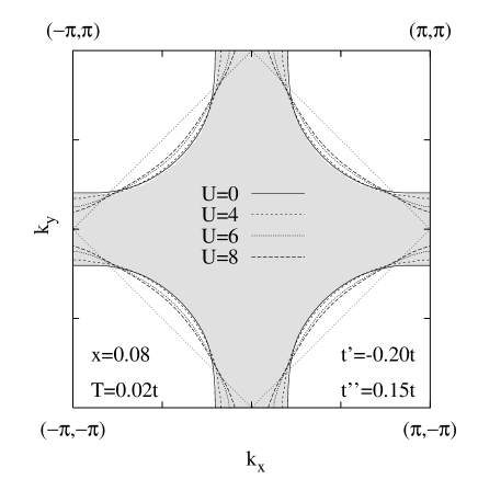
FIG. 1.: The Fermi-surface for different values of $U$ for fixed temperature $T=0.02t$ and hole doping $x=0.08$. The shaded area represents the states occupied by electrons.

FIG. 2.: Quasiparticle dispersions for the Fermi-surfaces shown in Fig. 1. We only show the most interesting flat part around $(\pi,0)$.

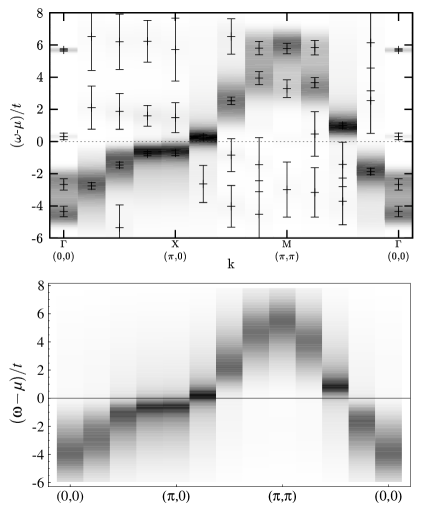
FIG. 3.: Spectral functions $A({\bf k},\omega)$ for $U=4t,t^{\prime}=-0.2t,t^{\prime\prime}=0.15t,x=0.08,T=0.33t$ as obtained by QMC (top) and MFLEX (bottom) on $8\times 8$ systems. Dark (bright) areas correspond to a large (low) spectral weight. Note that the energy dispersion depends weakly on the temperature.

FIG. 4.: (a) Static spin susceptibility $\chi_{zz}({\bf q},\omega=0)$ along the standard path in the Brillouin zone as obtained by MFLEX and QMC calculations. (b) Corresponding dynamical spin susceptibility ${\rm Im}\chi_{zz}({\bf Q},\omega)$ at the antiferromagnetic momentum ${\bf Q}=(\pi,\pi)$. All data are for $U=4t,t^{\prime}=-0.2t,t^{\prime\prime}=0.15t$ and a $8\times 8$ lattice except for the MFLEX results in (a), additionally labeled by $64^{2}$, which are for a $64\times 64$ system.

FIG. 5.: The inverse of the magnetic energy scale $\omega_{\rm sf}$ as a function of $U$ for various temperatures ($x=0.08,t^{\prime}=-0.2,t^{\prime\prime}=0.15$). A SDW instability manifests itself by $\omega_{\rm sf}\to 0$.

FIG. 6.: Same as Fig. 4, but for $U=8t$ and $x=0.10$.(a) Static spin susceptibility (b) Corresponding dynamical spin susceptibility

FIG. 7.: (a) $T_{1}T$ and (b) $T_{2G}$ NMR relaxation times calculated in the MFLEX approximation for $U/t=4.5$, $t^{\prime}/t=-0.2$, and $t^{\prime\prime}/t=0.15$, and two different doping levels, representing $\rm YBa_{2}Cu_{3}O_{6.63}$ ($x=0.08$) and $\rm YBa_{2}Cu_{3}O_{7}$ ($x=0.16$).

FIG. 8.: Static susceptibility in the Brillouin zone for $U=4.5t,x=0.08$ and $T=150{\rm K}$.Although this function is strongly peaked at ${\bf Q}=(\pi,\pi)$ indicating a commensurate spin response, it is better fitted by four incommensurate peaks.

FIG. 9.: Correlation length obtained by fitting the static susceptibility along the line from $(\pi,0)$ to $(\pi,\pi)$ with a superposition of 4 incommensurate Lorentzian-shaped peaks symmetrically located around ${\bf Q}$.

FIG. 10.: The magnetic energy scale $\omega_{\rm sf}$ defined to be the frequency where the dynamical susceptibility at ${\bf Q}$ is maximal.

- [1] S.-C. Zhang, Science 275, 1089 (1997).
- [2] R. Eder, W. Hanke, and S. C. Zhang, Phys. Rev. B 57, 13781 (1998).
- [3] S. Meixner, W. Hanke, E. Demler, and S.-C. Zhang, Phys. Rev. Lett. 79, 4902 (1997).
- [4] D. J. Scalapino, Physics Reports 250, 329 (1995).
- [5] A.J. Millis, H. Monien, and D Pines, Phys. Rev. B 42, 167 (1990).
- [6] D. Pines, Z. Phys. B 103, 129 (1997).
- [7] V. Barzykin and D. Pines, Phys. Rev. B 52, 13585 (1995).
- [8] Y. Zha, V. Barzykin and D. Pines, Phys. Rev. B 54, 7561 (1996).
- [9] Q. Si, Y. Zha, K. Levin, and J. P. Lu, Phys. Rev. B 47, 9055 (1993).
- [10] R. Preuss, W. Hanke, and W. von der Linden, Phys. Rev. Lett. 75, 1344 (1995).
- [11] D. Duffy, A. Nazarenko, S. Haas, A. Moreo, J. Riera, and E. Dagotto, cond-mat/9701083.
- [12] D. Duffy and A. Moreo, Phys. Rev. B 52, 15607 (1995).
- [13] R. Preuss, W. Hanke, C. Gröber, and H. G. Evertz, Phys. Rev. Lett. 79, 1122 (1997).
- [14] We measure the momenta in units of the lattice spacing.
- [15] Z.-X. Shen and D.S. Dessau, Phys. Rep. 255, 1 (1995).
- [16] C. Kim, P. J. White, Z.-X. Shen, T. Tohyama, Y. Shibata, S. Maewawa, B. O. Wells, Y. J. Kim, R. J. Birgeneau, and M. A. Kastner, Phys. Rev. Lett. 80, 4245 (1998).
- [17] R. Liu, B.W. Veal, A.P. Paulikas, J.W. Downey, P.J. Kostic, S. Flesher, U. Welp, C.G. Olson, X. Wu, A.J. Arko and J. Joyce, Phys. Rev. B 46, 11056 (1992).
- [18] D.S. Dessau, Z.-X. Shen, D.M. King, D.S. Marshall, L.W. Lombardo, P.H. Dickinson, J. DiCarlo, C.-H. Park, A.G. Loeser, A. Kapitulnik, and W.E. Spicer, Phys. Rev. Lett. 71, 2781 (1993).
- [19] D. S. Marshall, D. S. Dessau, A. G. Loeser, C.-H. Park, A. Y. Matsuura, J. N. Eckstein, I. Bozovic, P. F. A. Kapitulnik, W. E. Spicer, and Z.-X. Shen, Phys. Rev. Lett. 76, 4841 (1996).
- [20] T. Tohyama and S. Maekawa, Phys. Rev. B 49, 3596 (1994).
- [21] O. K. Andersen, A. I. Liechtenstein, O. Jepsen, and F. Paulsen, J. Phys. Chem. Solids 56, 1573 (1995).
- [22] V. I. Belinicher, A. L. Chernyshev, and V. A. Shubin, Phys. Rev. B 54, 14914 (1996).
- [23] T. Xiang and J. M. Wheatley, Phys. Rev. B 54, R12653 (1996).
- [24] R. Eder, Y. Ohta, and G. A. Sawatzky, Phys. Rev. B 55, R3414 (1997).
- [25] N. E. Bickers and D. J. Scalapino, Ann. Phys. 193, 206 (1989).
- [26] N. E. Bickers and S. R. White, Phys. Rev. B 43, 8044 (1991).
- [27] M. Langer, J. Schmalian, S. Grabowski, and K. H. Bennemann, Phys. Rev. Lett. 75, 4508 (1995).
- [28] G. Baym and L. P. Kadanoff, Phys. Rev. 124, 287 (1961); G. Baym, Phys. Rev. 127, 1391 (1962).
- [29] C.H. Pao and N.E. Bickers, Phys. Rev. B 49, 1586 (1994).
- [30] T. Dahm and L. Tewordt, Phys. Rev. B 52, 1297 (1995).
- [31] R. N. Silver, D. S. Sivia, and J. E. Goubernatis, Phys. Rev. B 41, 2380 (1990).
- [32] J. Schmalian, M. Langer, S. Grabowski, and K. H. Bennemann, Comp. Phys. Comm. 93, 141 (1996).
- [33] M.R. Presland, J.L Tallon, R.G. Buckley, R.S. Liu, and N.E. Flower , Physica C 176, 95 (1991).
- [34] D. Obertelli, J.R. Cooper, and J.L. Tallon, Phys. Rev. B 46, 14928 (1992); J.L. Tallon, C. Bernhard, H. Shaked, R.L. Hittermann, and J.D. Jorgenen Phys. Rev. B 51, 12911 (1995).
- [35] The effects of the electronic correlations, especially the antiferromagnetic fluctuations, on the temperature as well as the doping dependence of the thermoelectric power is discussed in G. Hildebrand, T.J. Hagenaars, W. Hanke, S. Grabowski, and J. Schmalian, Phys. Rev. B 56, R4317 (1997).
- [36] Z.-X. Shen and J. R. Schrieffer, Phys. Rev. Lett. 78, 1771 (1997).
- [37] Indications of a violation of Luttinger theorem, although at finite , have been found in J. Schmalian, M. Langer, S. Grabowski, and K.H. Bennemann, Phys. Rev. B 54, 4341 (1996).
- [38] We define the band dispersion by the maximum in of the spectral function for each .
- [39] R. Putz, R. Preuss, A. Muramatsu, and W. Hanke, Phys. Rev. B 53, 5133 (1996).
- [40] J. Altmann, W. Brenig, and A.P. Kampf, cond-mat/9707267.
- [41] T. Dahm and L. Tewordt, Phys. Rev. B 52, 1297 (1995).
- [42] N. Bulut, D.J. Scalapino, and S.R. White, Phys. Rev. B 47, 2742 (1993).
- [43] J. Rossat-Mignod, L.P. Regnault, C. Vettier, P. Bourges, P. Burlet, J. Jossy, J.Y. Henry and G. Lapertot, Physica C 185, 86 (1991).
- [44] H.F. Fong, B. Keimer, D.L. Milius, and I.A. Askay, Phys. Rev. Lett. 78, 713 (1997). B. Keimer, H.F. Fong, S.H. Lee, D.L. Milius, and I.A. Askay, Physica C 282, 232 (1997).
- [45] M. Horvatić, T. Auler, C. Berhier, Y. Berthier, P. Butaud, W.G. Clark, J.A. Gillet, P. Ségransan, and J.Y. Henry, Phys. Rev. B 47, R3461 (1993).
- [46] B. Shastry, Phys. Rev. Lett. 63, 1288 (1989). F. Mila and T.M. Rice, Physica C 157, 561 (1989).
- [47] D. Thelen and D. Pines Phys. Rev. B 49, 3528 (1994).
- [48] M. Takigawa, Phys. Rev. B 49, 4158 (1994).
- [49] N. Bulut, D.W. Hone, D.J. Scalapino, and N.E. Bickers, Phys. Rev. Lett. 64, 2723 (1990).
- [50] T. Imai, C. P. Slichter, A. P. Paulikas, and B. Veal, Phys. Rev. B 47, 9158 (1993).
- [51] M. Takigawa, Phys. Rev. B 49, 4158 (1994).
- [52] J. Fink, N. Nucker, E. Pellegrin, H. Romberg, M. Alexander, M. Knupfer, Journal of Electron Spectroscopy and Related Phenomena, High- special issue, 66, 395 (1994); H. Romberg, N. Nucker, J. Fink, T. Wolf, X.X. Xi, B. Koch, H.P. Geserich, M. Durrler, W. Assmus, B. Gegenheimer, Z. Phys. B 78, 367 (1990).
- [53] T.E. Mason, G. Aeppli, and H.A. Mook, Phys. Rev. Lett. 68, 1414 (1992); S.-W. Cheong, G. Aeppli, T.E. Mason, H. Mook, S.M. Hayden, P.C. Canfield, Z. Fisk, K.N. Clausen, and J.L. Marinez, Phys. Rev. Lett. 67, 1791 (1991).
- [54] E. Arrigoni and G. C. Strinati, Phys. Rev. B 44, 7455 (1991).
- [55] P. Bourges, L.P. Regnault, Y. Sidis, and C. Vettier, Phys. Rev. B 53, 876 (1996).
- [56] J.M. Tranquada, P.N. Gehring, G. Shirane, S. Shamoto, and M. Sato , Phys. Rev. B 46, 5561 (1992).
- [57] P. Dai, H.A. Mook, and F. Doğan, cond-mat/9707112.
- [58] P. Dai, H.A. Mook, and F. Doğan, cond-mat/9712311.