[

Weak selection and stability of localized distributions in Ostwald ripening

Abstract

We support and generalize a weak selection rule predicted recently for the self-similar asymptotics of the distribution function (DF) in the zero-volume-fraction limit of Ostwald ripening (OR). An asymptotic perturbation theory is developed that, when combined with an exact invariance property of the system, yields the selection rule, predicts a power-law convergence towards the selected self-similar DF and agrees well with our numerical simulations for the interface- and diffusion-controlled OR.

]

In a late stage of a first-order phase transition a two-phase mixture undergoes coarsening, or Ostwald ripening (OR), when the minority phase tends to minimize its interfacial energy under condition of a constant volume [2, 3, 4]. Despite numerous works, OR continues to attract attention both in experiment [5] and in theory [6, 7]. Our main motivation in studying this problem has been an attempt to resolve an old selection problem (described below) that created much controversy.

The “classical” formulation of the problem of OR, valid in the limit of a negligibly small volume fraction of the minority domains, is due to Lifshitz and Slyozov (LS) [2, 3] and Wagner [4]. In this formulation, the dynamics of the distribution function (DF) $F(R,t)$ of the domain sizes are governed (in scaled variables) by the continuity equation

$$\frac{\partial F}{\partial t}+\frac{\partial}{\partial R}(VF)=0\,,\quad V(R,t)=\frac{1}{R^{n}}\left(\frac{1}{R_{c}}-\frac{1}{R}\right)\,,$$ (1)

where $R_{c}(t)$ is the critical radius for expansion/shrinkage of an individual drop, while $n$ is determined by the mass transfer mechanism. The dynamics are constrained by conservation of the total volume of the minority domains:

$$\int_{0}^{\infty}R^{3}\,F(R,t)\,dR\,=Q=const\,.$$ (2)

Of great interest are possible self-similar intermediate asymptotics of this problem and the rule that selects the relevant asymptotics out of many possibilities. Scaling analysis of Eqs. (1) and (2) yields a similarity ansatz $F(R,t)=t^{-\mu}\,\Phi\,(R\,t^{-\nu})$ and $R_{c}=(t/\sigma)^{\nu}$, where $\mu=4/(n+2)$, $\nu=1/(n+2)$ and $\sigma=const$. Upon substitution, one finds a family of self-similar DFs for every $n\geq-1$, where each of the DFs is localized on a finite interval $[0,u_{m}]$ of the similarity variable $u=R\,t^{-\nu}$. The DFs can be parameterized by $\sigma$, and the interval of possible values of $\sigma$ is determined by the requirements of the continuity of $F(R,t)$ on the whole interval $[0,u_{m}]$ and normalizability with respect to Eq. (2). For each of the solutions, the average domain radius grows in time like $t^{1/(n+2)}$, and the number of domains decreases like $t^{-3/(n+2)}$, but the coefficients in these scaling laws are $\sigma$-dependent.

The self-similarity and related scalings were discovered by LS [2, 3] in the case of $n=1$ (diffusion-controlled OR). LS arrived at a unique self-similar DF (we will call it the limiting solution), and ruled out other possible solutions. In the first paper [2], the other solutions were rejected as non-normalizable with respect to Eq. (2). In the case of $n=0$ (interface-controlled OR) this argument was repeated by Wagner [4]. However, already in their second paper [3] on the same subject LS realized that no problem with normalization arises for initially localized DFs (that is, for those with a compact support at $t=0$). This correction was apparently overlooked in the literature (e.g., Ref. [8]), until Brown [9] addressed the other solutions and found them numerically for $n=1$. This created a long-standing controversy (see, e.g. [10]), and the first step towards resolving it was made in the case of $n=0$ [7]. It was noted that a DF, initially localized on an interval $[0,\,R_{m}(t=0)]$, always remains localized on a (time-dependent) interval $[0,\,R_{m}(t)]$. Furthermore, if $F(R,\,t=0)$ is describable by a power law $A_{0}\,[R_{m}(t=0)-R]^{\lambda}$ in the close vicinity of $R=R_{m}(t=0)$, then for any $t>0$ the leading term in the expansion of $F(R,\,t)$ in the vicinity of $R=R_{m}(t)$ has the form $A(t)\,[R_{m}(t)-R]^{\lambda}$. Invariance of the exponent $\lambda$ under the dynamics (1) and (2) implies a (weak) selection rule for the “correct” self-similar DF, as there is a one-to-one correspondence between $0<\lambda<+\infty$ and the parameter $\sigma$ [7]. [The limiting solution corresponds to an extended (non-compact) initial condition or, formally, to $\lambda\rightarrow+\infty$.] More precisely, if a self-similar asymptotics is ever reached, it must be the one selected by $\lambda$. However, no attempts have been made to solve (even numerically) the full time-dependent problem with a localized initial DF. Furthermore, no stability/convergence analysis for the localized DFs has been performed, so the selection rule proposed in [7] has remained unconfirmed.

This Letter supports the selection rule along three directions. The first one is to generalize the selection rule for any $n\geq-1$. The second is to prove the stability of and analyze the convergence towards the selected self-similar DF. The third is to verify our theoretical predictions numerically.

A meaningful formulation of the stability problem requires some care. Indeed, each member of the family of self-similar solutions for the DF, except the limiting solution, is formally unstable with respect to addition of an (infinite) tail. In this case it is the limiting solution that will finally develop [2, 3, 10]. However, such a perturbation is not always possible. In addition, the results of [7] imply that each member of the family, except the limiting solution, is formally unstable with respect to a localized perturbation that either has a larger $R_{m}$ than the “unperturbed” DF, or the same $R_{m}$ and a smaller exponent $\lambda$. In each of these cases another self-similar solution from the same family finally develops (as we see in our numerical simulations), and this situation can hardly be regarded as instability. A meaningful formulation of the stability problem should therefore deal with initial perturbations localized on the same interval of $R$ as the “unperturbed” DF, and characterized by the same exponent in the close vicinity of $R_{m}(t=0)$.

We will develop an asymptotic linear theory that, combined with an (exact) invariance property of the model, will enable us to prove, analytically, the stability of each of the self-similar DFs. This result and our numerical simulations will confirm the weak selection rule [7]. We will analyze the late-time convergence of an initially localized DF towards the selected self-similar DF and find a power-law decay in time for the corresponding (non-self-similar) perturbation. This decay is much faster than the logarithmic decay found for the limiting solution [2, 3]. We will see that not only the selected self-similar DF, but also the decay exponent are determined solely by the analytical properties of $F(R,t=0)$ in the close vicinity of $R_{m}(t=0)$. Our theoretical predictions show a very good agreement with simulations.

We will start with the asymptotic theory. Solving the problem analytically is made possible by a change of variables that employs the compactness of the support $[0,R_{m}(t)]$ of the DF. Introduce a scaled drop radius and a new time:

$$x(R,t)=\frac{R}{R_{m}(t)}\quad\mbox{and}\quad\tau=\int\limits_{0}^{t}\frac{dt^{\prime}}{R_{m}^{n+2}(t^{\prime})}\,,$$ (3)

and a scaled DF

$$G(x,\tau)=R_{m}^{4}[t(\tau)]\,F[R(x,\tau),t(\tau)]\,.$$ (4)

In the new variables Eqs. (1) and (2) can be rewritten as

$$(\partial G/\partial\tau)+\left[v\,(x^{-n}-x)+x-x^{-n-1}\right](\partial G/\partial x)$$ (5)

$$+\left[(n+1)x^{-n-2}-nvx^{-n-1}-4(v-1)\right]\,G=0$$ (6)

and $\int\limits_{0}^{1}G(x,\tau)x^{3}\,dx=Q\,,$ respectively, where $v(\tau)=R_{m}[t(\tau)]/R_{c}[t(\tau)]$. The function $G(x,\tau)$ is nonzero on the interval $0<x<1$ and zero elsewhere.

We will see in a moment that a self-similar solution for $F(R,t)$ corresponds to a steady-state solution for $G(x,\tau)$. Therefore, we are looking for the solution in the following form:

$$G(x,\tau)=\Phi_{0}(x)+\Phi_{1}(x)\,e^{q\tau}+\dots\ ,$$ (7)

$$v(\tau)=v_{0}+v_{1}\,e^{q\tau}+\dots\ ,$$ (8)

where $q$ is a (sought for) complex number. Both $\Phi_{0}(x)$, and $\Phi_{1}(x)$ are localized on the interval $[0,1]$. The perturbation must not change the normalization condition (2) and the asymptotics of the unperturbed solution near the point $x=1$, that is, $\int\limits_{0}^{1}x^{3}\,\Phi_{1}(x)\,dx=0$ and $\Phi_{1}={\cal O}(\Phi_{0})$ at $x\to 1$.

A family of steady-state solutions $\Phi_{0}(x)$ (parameterized by $v_{0}$) is obtained from the zero-order equation

$$\left[v_{0}\,(x^{-n}-x)+x-x^{-n-1}\right](d\Phi_{0}/dx)$$ (9)

$$+\left[(n+1)x^{-n-2}-nv_{0}x^{-n-1}-4(v_{0}-1)\right]\,\Phi_{0}=0\,.$$ (10)

Integration of this equation in elementary functions is possible for $n=-1,0,1$ and $2$ (that is, for most cases of physical interest [11]). For example, for $n=0$ one has

$$\Phi_{0}(x)=C_{Q}\,x\,(1-x)^{\alpha}\,(x_{2}-x)^{\nu}\,,\,\,0\leq x\leq 1\,,$$ (11)

where

$$\alpha=\frac{4v_{0}-5}{2-v_{0}}\ ,\quad\nu=\frac{v_{0}-5}{2-v_{0}}\ ,\quad x_{2}=\frac{1}{v_{0}-1}\ ,$$ (12)

while $C_{Q}$ is determined from the condition $\int\limits_{0}^{1}x^{3}\,\Phi_{0}(x)\,dx$ $=Q$. This family of solutions is defined for $5/4<v_{0}<2$. It corresponds to the family of self-similar solutions for $F(R,\,t)$ obtained in Ref. [7].

For $n=1$ one obtains

$$\Phi_{0}=C_{Q}x^{2}(1-x)^{\alpha}(x-x_{-})^{\gamma_{2}-\gamma_{1}}(x_{+}-x)^{-\gamma_{1}-\gamma_{2}}\,.$$ (13)

Here

$$\alpha=\frac{5v_{0}-6}{3-2v_{0}}\,,\quad\gamma_{1}=\frac{12-7v_{0}}{6-4v_{0}}\,,\quad\gamma_{2}=\frac{3v_{0}}{(6-4v_{0})s}\,,$$ (14)

$x_{\pm}=(-1\pm s)/2$, $s=[(v_{0}+3)/v_{0}-1)]^{1/2}$ and $0\leq x\leq 1$. This family is defined for $6/5<v_{0}<3/2$.

For any $n$, we will need to know the behavior of $\Phi_{0}(x)$ and $\Phi_{1}(x)$ in the close vicinity of $x=1$. A simple analysis of Eq. (10) yields $\Phi_{0}=H_{0}(\zeta)\,\zeta^{\alpha}\,$, where $\zeta=1-x$, $H_{0}(\zeta)$ is an analytic function on the interval $[0,1]$, $H_{0}(0)\neq 0$, and

$$\alpha=\frac{(n+4)\,v_{0}-n-5}{n+2-(n+1)\,v_{0}}\,.$$ (15)

The solution for $\Phi_{0}(x)$ exists if $0<\alpha<\infty$, that is $(n+5)/(n+4)<v_{0}<(n+2)/(n+1)$. This interval of permitted values of $v_{0}$ is non-empty for any $n\geq-1$. [The case of $n=-1$ is the simplest: $H_{0}(\zeta)=const$.]

Now we go to the first order in Eq. (6):

$$\left[v_{0}\,(x^{-n}-x)+x-x^{-n-1}\right](d\Phi_{1}/dx)$$ (16)

$$+\left[q-(n+1)x^{-n-2}-nv_{0}x^{-n-1}-4(v_{0}-1)\right]\,\Phi_{1}$$ (17)

$$=v_{1}\left[(x-x^{-n})\,(d\Phi_{0}/dx)+(4+nx^{-n-1})\Phi_{0}\right]\,.$$ (18)

For a given $v_{1}$, this linear equation can be solved in quadratures [12]. We will need only the leading asymptotics of the solution in the close vicinity of $x=1$, so we write down the solution as

$$\Phi_{1}=\zeta^{\alpha}\,\chi_{1}(\zeta)\,+\zeta^{\beta}\,\chi_{2}(\zeta)\,,$$ (19)

where $\beta=\alpha-q[n+2-(n+1)v_{0}]^{-1}$, $\chi_{1}$ and $\chi_{2}$ are analytic functions on the interval $[0,1]$ and $\chi_{1,2}\,(0)\neq 0$. The solution exists if $Re\,{\beta}\geq 0$ which implies $Re\,q<(n+4)v_{0}-n-5$. One can check a posteriori that this inequality holds.

Eq. (19) will be used later. At this stage we notice that the still undetermined “eigenvalue” $q$ must be selected by the initial condition. To make this selection possible, we should exploit an (exact) invariance property of Eq. (1). Consider the initial value problem $dR/dt=V(R,t)\,,R(0)=R_{0}$ that describes the characteristics of Eq. (1). If the solution of this problem, $R(t;R_{0})$, is known, the solution of Eq. (1) can be written in the following form:

$$F(R,t)=F_{0}[R_{0}(R,t)]\,\partial R_{0}(R,t)/\partial R,$$ (20)

where $R_{0}(R,t)$ is the function inverse to $R(t,R_{0})$ with respect to the argument $R_{0}$. Now, $R(t,R_{0})$ is an analytic and monotonic function of $R_{0}$. Therefore, the inverse function $R_{0}(R,t)$ is also an analytic function of $R$, and so $F(R,t)$ preserves its analytic form along the characteristics $R=R(t;R_{0})$, including the “edge” characteristics $R_{m}(t)$.

We assume a power-law behavior of $F(R,\,t=0)$ in the close vicinity of $R=R_{m}(0)$. More precisely, we assume that

$$F_{0}(\xi)=\xi^{\lambda_{1}}g_{1}(\xi)+\xi^{\lambda_{2}}g_{2}(\xi)\,,$$ (21)

where $\xi=R_{m}(0)-R>0$. Here $\lambda_{1}$ and $\lambda_{2}>\lambda_{1}$ are arbitrary positive numbers, such that $\lambda_{2}-\lambda_{1}\neq 1,\,2,\,\dots\,$, and $g_{1}(\xi)$ and $g_{2}(\xi)$ are analytic at $\xi=0$ such that $g_{1,2}(0)\neq 0$. In view of of the analyticity property mentioned above, Eq. (20) can be rewritten as

$$F(R,t)=(\xi^{\prime})^{\lambda_{1}}h_{1}(\xi^{\prime},t)+(\xi^{\prime})^{\lambda_{2}}h_{2}(\xi^{\prime},t)\,,$$ (22)

where $\xi^{\prime}=R_{m}(t)-R>0$, while $h_{1}(\xi^{\prime},t)$ and $h_{2}(\xi^{\prime},t)$ are analytic functions of $\xi^{\prime}$ at $\xi^{\prime}=0$, and $h_{1,2}(0,t)\neq 0$.

Under the transformation (3), (4) the variables $R$ and $F$ are multiplied by some quantities independent of $R$. Therefore, we can rewrite Eqs. (21) and (22) in the new variables $x$ and $\tau$ as follows. The initial DF is now

$$G_{0}(x)=\zeta^{\lambda}_{1}\,g^{\prime}_{1}(\zeta)+\zeta^{\lambda_{2}}\,g^{\prime}_{2}(\zeta)\,,\quad\quad\zeta>0,$$ (23)

where $g^{\prime}_{1}(\zeta)$ and $g^{\prime}_{2}(\zeta)$ are analytic at $\zeta=0$, $g^{\prime}_{1,2}(0)\neq 0$, and we remind that $\zeta=1-x$. Correspondingly, the time-dependent DF $G(x,\tau)$ can be written as

$$G(x,\tau)=\zeta^{\lambda_{1}}\,h^{\prime}_{1}(\zeta,\tau)+\zeta^{\lambda_{2}}\,h^{\prime}_{2}(\zeta,\tau)\,,\quad\quad\zeta>0,$$ (24)

where $h^{\prime}_{1}(\zeta,\tau)$ and $h^{\prime}_{2}(\zeta,\tau)$ are analytic functions of $\zeta$ in $\zeta=0$, and $h^{\prime}_{1,2}(0,\tau)\neq 0$.

The exponents $\lambda_{1}$ and $\lambda_{2}$, prescribed by the initial conditions, remain invariant. Hence, the long-time asymptotics of Eq. (24) should coincide with that given by Eqs. (8) and (19). A direct comparison yields $\alpha=\lambda_{1}$ and $\beta=\lambda_{2}$. The first equality is nothing but a (weak) selection rule for the self-similar solution, and the selected value of $v_{0}$ is

$$v_{0}=\frac{(n+2)\lambda_{1}+n+5}{(n+1)\lambda_{1}+n+4}\,.$$ (25)

The second equality determines $q$:

$$-q=\frac{3(\lambda_{2}-\lambda_{1})}{(n+1)\lambda_{1}+n+4}\,.$$ (26)

One can see that $-q$ is real and positive which means stability.

Going back to the “physical” variables $R$ and $t$ is easy. Indeed, evaluating $R_{m}(t)$ on the self-similar solution, we obtain $R_{m}(t)=\left[(n+2)\,(v_{0}-1)\,t\right]^{1/(n+2)}.$ Then, using Eq. (3), we see that $e^{q\tau}=t^{-\Gamma}$, a power-law decay in the “physical” time. Here

$$\Gamma=\frac{3(\lambda_{2}-\lambda_{1})}{(n+2)(\lambda_{1}+1)}>0\,.$$

If we limit ourselves to an important particular case of a single “non-trivial” exponent in the initial DF, $G_{0}(x)=\zeta^{\lambda}g(\zeta)$, [where $g(\zeta)$ is analytic and $g(0)\neq 0$], then $G(x,\tau)=\zeta^{\lambda}h(\zeta,\tau)$, where $h(\zeta,\tau)$ is an analytic functions of $\zeta$ and $h(0,\tau)\neq 0$. Now, using Eqs. (8) and (19), we obtain

$$-q=\frac{3}{(n+1)\lambda+n+4}\,,$$ (27)

unless the linear term in the Taylor series of $g(\zeta)$ at $\zeta=0$ vanishes [13]. This yields the power exponent

$$\Gamma=\frac{3}{(n+2)(\lambda+1)}\,.$$ (28)

In the limit of $\lambda\to\infty\,$, we obtain $\Gamma\to 0$. Clearly, it corresponds to the logarithmically slow decay obtained for the limiting solution [2, 3].

Therefore, both the self-similar DF, and the power-law decay rate of a small perturbation around it are uniquely determined by the asymptotics of the initial DF in the close vicinity of the maximum domain size, $R=R_{m}(0)$.

We verified the theory (in the cases $n=0$ and $1$) by performing extensive numerical simulations with Eq. (1) and an explicit equation for $\dot{R_{c}}$ that follows from Eqs. (1) and (2). As the dynamics is extremely sensitive to small changes in the vicinity of $R=R_{m}(t)$, we needed an algorithm that preserved the compactness of the DF and kept a high accuracy near the edge point $R=R_{m}(t)$. A simple and efficient Lagrangian algorithm was developed [14] that satisfied these requirements. Typical simulation results for the interface-controlled OR, $n=0$, are presented in Figs. 1 and 2. Figure 1 shows convergence of an initially localized DF, $F(R,0)=R\,(5-R)^{\lambda}$ with $\lambda=1$, towards the selected self-similar DF (11), for which Eq. (25) predicts $v_{0}=7/5$. The inset shows convergence of $v(t)$ towards $v_{0}=7/5$. The convergence exponent $\Gamma_{exp}=0.76$ found numerically agrees very well with our theoretical prediction $\Gamma_{th}=0.75$. Figure 2 shows the convergence exponents $\Gamma_{exp}$ found numerically for different $\lambda$. A good agreement with the theoretical curve $\Gamma_{th}=3/[2(\lambda+1)]$ is seen. We also observed a good agreement between the theory and simulations in the case of the diffusion-controlled OR, $n=1$.

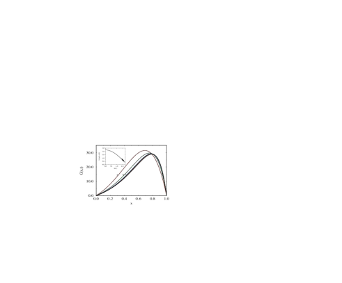
FIG. 1.: Convergence of an initially localized DF with $\lambda=1$ towards the selected self-similar DF (11) with $v_{0}=7/5$ (solid line). Numerical solutions are shown by dotted lines at time moments $t=20$ (a), $100$ (b), $500$ (c) and 1000. The inset shows the convergence of $v(t)$ towards $v_{0}=7/5$.

We have demonstrated that only a weak selection is possible in the “classical” model of OR. To get a strong selection rule, one obviously must go beyond the “classical” model.

This work was supported in part by a grant from Israel Science Foundation, administered by the Israel Academy of Sciences and Humanities, and by the Russian Foundation for Basic Research (grant No. 96-01-01876).

FIG. 2.: Convergence exponents predicted analytically (line) and found numerically (squares) for different $\lambda$.

REFERENCES

- [1] On leave from the Institute of Theoretical and Experimental Physics, Moscow 117259, Russia.
- [2] I.M. Lifshitz and V.V. Slyozov, Zh. Exp. Teor. Fiz. 35, 479 (1958) [Sov. Phys. JETP 8, 331 (1959)].
- [3] I.M. Lifshitz and V.V. Slyozov, J. Phys. Chem. Solids 19, 35 (1961).
- [4] C. Wagner, Z. Electrochem. 65, 581 (1961).
- [5] O. Krichevsky and J. Stavans, Phys. Rev. E 52, 1818 (1995); W. Theis, N.C. Bartelt, and R.M. Tromp, Phys. Rev. Lett. 75, 3328 (1995); J.-M. Wen et al., Phys. Rev. Lett. 76, 652 (1996); K. Morgenstern, G. Rosenfeld and G. Comsa, Phys. Rev. Lett. 76, 2113 (1996); G.R. Carlow and M. Zinke-Allmang, Phys. Rev. Lett. 78, 4601 (1997); J.B. Hannon et al., Phys. Rev. Lett. 79, 2506 (1997).
- [6] M. Marder, Phys. Rev. A 36, 858 (1987); J.H. Yao et al., Phys. Rev. B 47, 14110 (1993); A.J. Bray, Adv. Phys. 43, 357 (1994); N. Akaiwa and P.W. Voorhees, Phys. Rev. E 49, 3860 (1994); V.G. Karpov, Phys. Rev. Lett. 74, 3185; 75, 2702 (1995); N. Akaiwa and D.I. Meiron, Phys. Rev. E 54, R13 (1996); C. Sagui, D.S. O’Gorman and M. Grant, Phys. Rev. E 56, R21 (1997).
- [7] B. Meerson and P.V. Sasorov, Phys. Rev. E 53, 3491 (1996).
- [8] E.M. Lifshitz and L.P. Pitaevsky, Physical Kinetics (Pergamon, London, 1981).
- [9] L.C. Brown, Acta Metall. 37, 71 (1989); Scripta Metall. Mater. 24, 963; 2231 (1990).
- [10] M.K. Chen and P.W. Voorhees, Modelling Simul. Mater. Sci. Eng. 1, 591 (1993).
- [11] V.V. Slyozov and V.V. Sagalovich, Sov. Phys. Usp. 30, 23 (1987); M. Zinke-Allmang, L.C. Feldman, and M.H. Grabow, Surf. Sci. Rep. 16, 377 (1992).
- [12] The solution is obtained by making the ansatz and directly solving the equation for .
- [13] If it does vanish, an additional factor 2 appears in the numerators of the right hand sides of Eqs. (27) and (28). In general, if is the order of the first non-vanishing term in the Taylor series, an additional factor appears.
- [14] B. Giron, Localized Distributions in the Problem of Ostwald Ripening, M.Sc. thesis, Hebrew University, Jerusalem (1998).