Superconductivity in Ultrasmall Metallic Grains

Abstract

We develop a theory of superconductivity in ultrasmall (nm-scale) metallic grains having a discrete electronic eigenspectrum with mean level spacing $d\simeq\tilde{\Delta}$ (bulk gap). The theory is based on calculating the eigenspectrum using a generalized BCS variational approach, whose (qualitative) applicability has been extensively demonstrated in studies of pairing correlations in nuclear physics. We discuss how conventional mean field theory breaks down with decreasing sample size, how the so-called blocking effect (the blocking of pair-scattering by unpaired electrons) weakens pairing correlations in states with non-zero total spin (thus generalizing a parity effect discussed previously), and how this affects the discrete eigenspectrum’s behavior in a magnetic field, which favors non-zero total spin. In ultrasmall grains, spin magnetism dominates orbital magnetism, just as in thin films in a parallel field; but whereas in the latter the magnetic-field induced transition to a normal state is known to be first-order, we show that in ultrasmall grains it is softened by finite size effects. Our calculations qualitatively reproduce the magnetic-field dependent tunneling spectra for individual aluminum grains measured recently by Ralph, Black and Tinkham [Phys. Rev. Lett. 78, 4087 (1997)]. We argue that previously-discussed parity effects for the odd-even ground state energy difference are presently not observable for experimental reasons, and propose an analogous parity effect for the pair-breaking energy that should be observable provided that the grain size can be controlled sufficiently well. Finally, experimental evidence is pointed out that the dominant role played by time-reversed pairs of states, well-established in bulk and in dirty superconductors, persists also in ultrasmall grains.

]

I Introduction

What happens to superconductivity when the sample is made very, very small? Anderson [1] addressed this question already in 1959: he argued that if the sample is so small that its electronic eigenspectrum becomes discrete, with a mean level spacing $d=1/{\cal N}(\varepsilon_{F})\sim 1/\mbox{Vol}$, “superconductivity would no longer be possible” when $d$ becomes larger than the bulk gap $\tilde{\Delta}$. Heuristically, this is obvious (see Fig. 1 below): $\tilde{\Delta}/d$ is the number of free-electron states that pair-correlate (those with energies within $\tilde{\Delta}$ of $\varepsilon_{F}$), i.e. the “number of Cooper pairs” in the system; when this becomes ${\stackrel{{\scriptstyle\scriptscriptstyle<}}{{\scriptscriptstyle\sim}}}1$, it clearly no longer makes sense to call the system “superconducting”.

Giaver and Zeller[2, 3] were among the first to probe Anderson’s criterion experimentally: studying tunneling through granular thin films containing electrically insulated Sn grains, they demonstrated the existence of an energy gap for grain sizes right down to the critical size estimated by Anderson (radii of $25$Å in this case), but were unable to prove that smaller particles are always normal. Their concluding comments are remarkably perspicuous:[3] “There can be no doubt, however, that in this size region the bulk theory of superconductivity loses its meaning. As a matter of fact, perhaps we should not even regard the particles as metallic because the energy-level spacing is large compared to $kT$ and because there are very few electrons at the Fermi surface. The question of the lower size limit for superconductivity is, therefore, strongly correlated with the definition of superconductivity itself.”

These remarks indicate succinctly why the study of superconductivity near its lower size limit is of fundamental interest: the conventional bulk BCS approach is not directly applicable, and some basic elements of the theory need to be rethought, with the role of level discreteness demanding special attention.

First steps in this direction were taken by Strongin et al.[4] and by Mühlschlegel et al.[5], who calculated the thermodynamic properties of small superconducting grains. However, since experiments at the time were limited to studying ensembles of small grains (e.g. granular films), there was no experimental incentive to develop a more detailed theory for an individual ultrasmall superconducting grain, whose eigenspectrum, for example, would be expected to reveal very directly the interplay between level discreteness and pairing correlations.

This changed dramatically in 1995, when Ralph, Black and Tinkham (RBT) [6] succeeded in constructing a single-electron transistor (SET) whose island was an ultrasmall metallic grain: by studying the tunneling current through the device, they achieved the first measurement of the discrete eigenspectrum of a single grain. This enabled them to probe the effects of spin-orbit scattering,[7, 8] non-equilibrium excitations[9] and superconductivity,[7, 9] which manifests itself through the presence (absence) of a substantial spectral gap in grains with an even (odd) number of electrons.

RBT’s work stimulated several theoretical investigations. Besides discussing non-equilibrium effects,[10, 11] these focused mainly on superconductivity,[12, 13, 14, 15, 16] and revealed that the breakdown of pairing correlations with decreasing grain size predicted by Anderson harbors some surprises when scrutinized in more detail: von Delft et al.[12] showed that this breakdown is affected by the parity ($p$) of the number of electrons on the grain: using parity-projected mean-field theory[17, 18] and variational methods and assuming uniformly spaced electron levels, they solved the parity-dependent gap equation for the even or odd ground state pairing parameters $\Delta_{e}$ or $\Delta_{o}$ as function of $d$ (using methods adapted from Strongin et al.[4]), and found that $\Delta_{o}(d)<\Delta_{e}(d)$, i.e. ground state pairing correlations break down sooner with increasing $d$ in an odd than an even grain (the difference becoming significant for $d\simeq\tilde{\Delta}$). This is due to the so-called blocking effect:[19] the odd grain always has one unpaired electron, which blocks pair-scattering of other pairs and thereby weakens pairing correlations. Smith and Ambegaokar[13] showed that this parity effect holds also for a random distribution of level spacings (as also anticipated by Blanter[20]), and Matveev and Larkin[14] investigated a parity effect occuring in the limit $d\gg\tilde{\Delta}$.

The $\Delta_{o}<\Delta_{e}$ parity effect has an obvious generalization, studied by Braun et al.[15] using a generalized BCS variational approach due to Soloviev:[19] any state with non-zero spin $s$ (not just the odd ground state) experiences a significant reduction in pairing correlations, since at least $2s$ electrons are unpaired, leading to an enhanced blocking effect ($\Delta_{s}<\Delta_{s^{\prime}}$ if $s>s^{\prime}$). The latter’s consequences can be observed in the magnetic-field dependence of SET tunneling spectra, since a magnetic field favors states with non-zero spin and consequent enhanced blocking effect. In ultrasmall grains, spin magnetism dominates orbital magnetism, just as in thin films in a parallel field;[21] but whereas in the latter the magnetic-field induced transition to a normal state is known to be first-order, Braun et al. showed that in ultrasmall grains the transition is softened due to finite size effects. Moreover, they argued that some of RBT’s grains fall in a region of “minimal superconductivity”, in which pairing correlations measurably exist at $H=0$, but are so weak that they may be destroyed by the breaking of a single pair (since the number of electron pairs that take part in the formation of a correlated state becomes of order one for $d\simeq\tilde{\Delta}$).

In the present paper we elaborate the methods used and results found by Braun et al. in Ref. [15] and present a detailed theory of superconductivity in ultrasmall grains. Our discussion can be divided into two parts: in the first (sections II and III), we consider an isolated ultrasmall grain and (a) define when and in what sense it can be called “superconducting”; (b) use a generalized BCS variational approach to calculate the eigenenergies of various variational eigenstates of general spin $|s\rangle$, which illustrates the break-down of mean-field theory; and (c) discuss how an increasing magnetic field induces a transition to a normal paramagnetic state. In the second part (section IV), we consider the grain coupled to leads as in RBT’s SET experiments and discuss observable quantities: (a) We calculate theoretical tunneling spectra of the RBT type, finding qualitative agreement with RBT’s measurements; (b) point out that the above-mentioned ground state energy parity effect can presently not be observed, and propose an analogous pair-breaking energy parity effect that should be observable in experiments of the present kind; and (c) explain how RBT’s experiments give direct evidence for the dominance of time-reversed pairing, at least for small fields (implying that the sufficiency of using only a reduced BCS-Hamiltonian, well-established for bulk systems and dirty superconductors, holds for ultrasmall grains, too).

II Pairing Correlations at fixed Particle Number

The discrete energies measured in RBT’s experiments essentially correspond to the eigenspectrum of a grain with fixed electron number $N$ (for reasons explained in detail in section IV A). In this and the next section, we therefore consider an ultrasmall grain completely isolated from the rest of the world, e.g. by infinitely thick oxide barriers.

When considering a truly isolated superconductor (another example would be a superconductor levitating in a magnetic field due to the Meissner effect) one needs to address the question: How is one to incorporate the fixed-$N$ condition into BCS theory, and how important is it to do so? Although this issue is well understood and was discussed at length in the early days of BCS theory, in particular in its application to pairing correlations in nuclei [22, p. 439], for pedagogical reasons the arguments are worth recapitulating in the present context. We shall first recall that the notion of pair-mixing [12] that lies at the heart of BCS theory is by no means inherently grand-canonical and can easily be formulated in canonical language, then summarize what has been learned in nuclear physics about fixed-$N$ projection techniques, and finally conclude that for present purposes, standard grand-canonical BCS theory should be sufficient. Readers familiar with the relevant arguments may want to skip this section.

A Canonical Description of Pair-Mixing

Conventional BCS theory gives a grand-canonical description of the pairing correlations induced by the presence of an attractive pairing interaction such as the reduced BCS interaction

$$H_{red}=-\sum_{jj^{\prime}}Vc^{\dagger}_{j+}c^{\dagger}_{j-}c_{j^{\prime}-}c_{j^{\prime}+}\;\quad(\mbox{with}\;V>0).$$ (1)

(The $c_{j\pm}$ are electron destruction operators for the single-particle states $|j,\pm\rangle$, taken to be time-reversed copies of each other, with energies $\varepsilon_{j\pm}$.) The theory employs a grand-canonical ensemble, formulated on a Fock space of states in which the total particle number $N$ is not fixed, as illustrated by BCS’s variational ground state Ansatz

$$|BCS\rangle=\prod_{j}(u_{j}+v_{j}c^{\dagger}_{j+}c^{\dagger}_{j-})\,|\mbox{Vac}\rangle\;\quad(u^{2}_{j}+v^{2}_{j}=1).$$ (2)

This is not an eigenstate of the number operator $\hat{N}=\sum_{j\sigma}c^{\dagger}_{j\sigma}c_{j\sigma}$ and its particle number is fixed only on the average by the condition $\langle BCS|\hat{N}|BCS\rangle=N$, which determines the grand-canonical chemical potential $\mu$. Likewise, the commonly used definition

$$\Delta_{BCS}=V\sum_{j}\langle c_{j+}c_{j-}\rangle\;$$ (3)

for the superconducting order parameter only makes sense in a grand-canonical ensemble, since it would trivially give zero when evaluated in a canonical ensemble, formulated on a strictly fixed-$N$ Hilbert space of states.

A theory of strictly fixed-$N$ superconductivity must therefore entail modifications of conventional BCS theory. In particular, a construction different from $\Delta_{BCS}$ is needed for the order parameter, which we shall henceforth call “pairing parameter”, since “order parameter” carries the connotation of a phase transition, which would require the thermodynamic limit $N\to\infty$. The pairing parameter should capture in a canonical framework BCS’s essential insight about the nature of the superconducting ground state: an attractive pairing interaction such as $H_{red}$ will induce pairing correlations in the ground state that involve pair-mixing across $\varepsilon_{F}$ (see also Ref. [12]), i.e. a non-zero amplitude to find a pair of time-reversed states occupied above $\varepsilon_{F}$ or empty below $\varepsilon_{F}$. BCS chose to express this insight through the Ansatz (2), which allows $v_{j}\neq 0$ for $\varepsilon_{j}>\varepsilon_{F}$ and $u_{j}\neq 0$ for $\varepsilon_{j}<\varepsilon_{F}$. It should be appreciated, however (and is made clear on p. 1180 of their original paper [23]), that they chose a grand-canonical construction purely for calculational convenience (the trick of using commuting products in (2) makes it brilliantly easy to determine the variational parameters $u_{j}$, $v_{j}$), and proposed themselves to use its projection to fixed $N$, $|BCS\rangle_{N}$, as the actual ground state.

Since $[H_{red},\hat{N}]=0$, one would expect that the essence of BCS theory, namely the presence of pair-mixing and the reason why it occurs, can also be formulated in a canonically meaningful way. Indeed, this is easy: pair-mixing is present if the amplitude $\bar{v}_{j}\equiv\langle c^{\dagger}_{j+}c^{\dagger}_{j-}c_{j-}c_{j+}\rangle^{1/2}$ to find a pair of states occupied is non-zero also for $\varepsilon_{j}>\varepsilon_{F}$, and the amplitude $\bar{u}_{j}\equiv\langle c_{j-}c_{j+}c^{\dagger}_{j+}c^{\dagger}_{j-}\rangle^{1/2}$ to find a pair of states empty is non-zero also for $\varepsilon_{j}<\varepsilon_{F}$ (the bars indicate that the $\bar{u}_{j}$ and $\bar{v}_{j}$ defined here differ in general from the $u_{j}$ and $v_{j}$ used by BCS; note, though, that the former reduce to the latter if evaluated using $|BCS\rangle$). The intuitive reason why $H_{red}$ induces pair-mixing in the exact ground states $|G\rangle$ despite the kinetic energy cost incurred by shifting pairing amplitude from below to above $\varepsilon_{F}$, is that this frees up phase space for pair-scattering, thus lowering the ground state expectation value of $H_{red}$: in $\langle G|H_{red}|G\rangle$, the $jj^{\prime}$ term can be non-zero only if both $c^{\dagger}_{j+}c^{\dagger}_{j-}c_{j^{\prime}-}c_{j^{\prime}+}|G\rangle\neq 0$, implying $(\bar{v}_{j^{\prime}})_{G}\neq 0$ and $(\bar{u}_{j})_{G}\neq 0$, and also $\langle G|c^{\dagger}_{j+}c^{\dagger}_{j-}c_{j^{\prime}-}c_{j^{\prime}+}\neq 0$, implying $(\bar{v}_{j})_{G}\neq 0$ and $(\bar{u}_{j^{\prime}})_{G}\neq 0$. By pair-mixing, the system can arrange for a significant number of states to simultaneously have both $(\bar{v}_{j})_{G}\neq 0$ and $(\bar{u}_{j})_{G}\neq 0$; this turns out to lower the ground state energy sufficiently through $\langle G|H_{red}|G\rangle$ that the kinetic energy cost of pair-mixing is more than compensated. Furthermore, an excitation that disrupts pairing correlations in the ground state by “breaking up a pair” will cost a finite amount of energy by blocking pair-scattering involving that pair. For example, the energy cost of having $|j+\rangle$ definitely occupied ($\bar{u}_{j}=0$) and $|j-\rangle$ definitely empty ($\bar{v}_{j}=0$) is

$\displaystyle\varepsilon_{j}(1-\langle G|\sum_{\sigma}c^{\dagger}_{j\sigma}c_{j\sigma}|G\rangle)+V\langle G|c^{\dagger}_{j+}c^{\dagger}_{j-}\!\!\sum_{j^{\prime}\neq j}c_{j^{\prime}-}c_{j^{\prime}+}|G\rangle,$

in which the restricted sum reflects the blocking of scattering involving the $j$-th pair. When evaluated using $|BCS\rangle$, this quantity reduces to $\varepsilon_{j}(1-2v_{j}^{2})+u_{j}v_{j}\Delta_{BCS}=[\varepsilon_{j}^{2}+\Delta_{BCS}^{2}]^{1/2}$, which is the well-known quasi-particle energy of the state $\gamma^{\dagger}_{j+}|BCS\rangle$.

The above simple arguments illustrate that there is nothing inherently grand-canonical about pair-mixing. Indeed, at least two natural ways suggest themselves to measure its strength in a canonically meaningful way, using for instance the pairing parameter $\bar{\Delta}\equiv V\sum_{j}\bar{u}_{j}\bar{v}_{j}$ proposed in Ref. [12], or one proposed by Ralph [24]:

$$\bar{\Delta}^{\prime}\equiv V\sum_{j}\left[\langle c^{\dagger}_{j+}c_{j+}c^{\dagger}_{j-}c_{j-}\rangle-\langle c^{\dagger}_{j+}c_{j+}\rangle\langle c^{\dagger}_{j-}c_{j-}\rangle\right]^{1/2}\!\!.$$ (4)

Both $\bar{\Delta}$ and $\bar{\Delta}^{\prime}$ were constructed such that they reduce, as is desirable, to the same result as $\Delta_{BCS}$ when each is evaluated using $|BCS\rangle$ with real coefficients $u_{j},v_{j}$, namely $V\sum_{j}u_{j}v_{j}$. An appealing feature of $\bar{\Delta}^{\prime}$ is that by subtracting out $\langle c^{\dagger}_{j+}c_{j+}\rangle\langle c^{\dagger}_{j-}c_{j-}\rangle$, it transparently emphasizes the pairing nature of superconducting correlations, i.e. the fact that if $|j+\rangle$ is empty (or filled), so is $|j-\rangle$: $\bar{\Delta}^{\prime}$ will be very small if the occupation of $|j+\rangle$ is uncorrelated with that of $|j-\rangle$, as it is in a normal Fermi liquid. The overall behavior (as function of energy $\varepsilon_{j}$) of the summands in both $\bar{\Delta}$ and $\bar{\Delta}^{\prime}$ will be similar to that of $u_{j}v_{j}$ (though not identical to $u_{j}v_{j}$ or to each other; a quantitative evaluation of the differences, which increase with increasing $d/\tilde{\Delta}$, requires an honest canonical calculation[25]). $u_{j}v_{j}$ is shown in Fig. 1(a), which illustrates that pair-mixing correlations are strongest within a region of width $\Delta_{BCS}$. In this paper, we shall call a system “pair-correlated” if $\bar{\Delta}^{\prime}$ is a significant fraction of its bulk value $\tilde{\Delta}$ (say, somewhat arbitrarily, at least 25%), and regard this as being synonymous with “superconducting”.

B On the breaking of Gauge Symmetry

In some discussions of conventional BCS theory the defining feature of superconductivity is taken to be the breaking of gauge symmetry by the order parameter. This concept is illustrated by the BCS order parameter $\Delta_{BCS}$ of Eq. (3): if non-zero, it has a definite phase and is not gauge-invariant (under $c_{j\sigma}\to e^{i\phi}c_{j\sigma}$, it changes to $e^{i2\phi}\Delta_{BCS}$). Note, though, that this point of view cannot be carried over to fixed-$N$ systems. Firstly, these trivially have $\Delta_{BCS}=0$, and secondly and more fundamentally, the breaking of gauge symmetry necessarily presupposes a grand-canonical ensemble: since phase and particle number are quantum-mechanically conjugate variables, formal considerations dictate that the order parameter acquire a definite phase only if the particle number is allowed to fluctuate, i.e. in a grand-canonical ensemble.

Of course, in certain experimental situations where $N$ manifestly does fluctuate, such as the celebrated Josephson effect of two superconductors connected by a tunnel junction, their order parameters do acquire definite phases, and their phase difference is a measurable quantity. However, for a truly isolated superconductor with fixed $N$ the “phase of the order parameter” is not observable, and the concept of gauge symmetry breaking through an order parameter with a definite phase ceases to be useful. Indeed, the canonically meaningful pairing parameters $\bar{\Delta}$ and $\bar{\Delta}^{\prime}$ defined above are manifestly gauge-invariant.

C Fixed-$N$ Projections

It is easy to construct a variational ground state exhibiting pair-mixing and having definite particle number, by simply projecting $|BCS\rangle$ to fixed $N$, as suggested by BCS [23]. This can be achieved by the projection integral

$$|BCS\rangle_{N}\equiv\!\int_{0}^{2\pi}\!\!\!\!\!\!d\phi\,e^{-i\phi N}\!\prod_{j}(u_{j}\!+\!e^{2i\phi}v_{j}c^{\dagger}_{j+}c^{\dagger}_{j-})\,|\mbox{Vac}\rangle,$$ (5)

whose randomization of the phases of the $v_{j}$’s illustrates, incidentally, why gauge invariance is not broken at fixed $N$.

This and related fixed-$N$ projections were studied in great detail in nuclear physics, with the aim of variationally calculating nuclear excitation spectra for finite nuclei ($N\leq 240$) exhibiting pairing correlations (Ring and Schuck provide an excellent review of the extensive literature, see chapter 11 of Ref. [22]; a recent reference is [26]). The simplest approach is called “projection after variation”: the unprojected expectation value $\langle BCS|H|BCS\rangle$ is minimized with respect to the variational parameters $\{v_{j}\}$, which thus have their standard BCS values $v_{j}^{2}={1\over 2}[1-\varepsilon_{j}/(\varepsilon_{j}^{2}+\Delta^{2}_{BCS})^{1/2}]$, but then these are inserted into $|BCS\rangle_{N}$ and expectation values evaluated with the latter instead of $|BCS\rangle$. This elimination of “wrong-$N$” states after variation turns out to lower the ground state energy relative to the unprojected case (by a few percent in nuclei) and thus improves the trial wave-function. Further improvements are possible using the more sophisticated “projection before variation” strategy, where the projected expectation value ${}_{N}\langle BCS|H|BCS\rangle_{N}$ is minimized with respect to the $\{v_{j}\}$. However, these then no longer have the simple BCS form, but instead are determined through a set of coupled relations, each involving all the other $v_{j}^{\prime}$s, that have to be solved numerically. The corrections $\delta v_{j}$ to the BCS pair-occupation amplitudes so produced further lower the ground state energy relative to projection after variation (but only by tenths of a percent).

Extensive applications of such and related approaches in nuclear physics have led to the following conclusions: For reasonably small $N$, as in nuclei, the explicit implementation of projection techniques is tractable, though cumbersome. For very large $N$ they become intractable, but also unnecessary, since their corrections can be shown to vanish as $N^{-1/2}$. However, even in nuclei the corrections to unprojected BCS theory are small (a few percent) in most cases, the only exception being very large couplings $V\geq d$. Thus, in most cases fixed-$N$ systems can perfectly adequately be described by BCS’s grand-canonical wave function. Its $N$-indefiniteness (and the associated breaking of gauge symmetry) then simply has the status of a clever calculational trick: it allows the use of a wave function so simple that the pair-occupation amplitudes $v_{j}$ can be found with a minimum of effort. The trick’s justification is that the corrections $\delta v_{j}$’s produced by more careful approaches usually are small. (The device of using symmetry-breaking wave-functions purely for the sake of calculational convenience is widespread in nuclear physics, and lucidly discussed in Ring and Schuck’s book[22] in a chapter entitled “Restoration of Broken Symmetries”.)

The above conclusions imply that the following strategy should suffice for a qualitative description (more is not attempted here) of pairing correlations in isolated ultrasmall grains: although strictly speaking a fixed-$N$ technique would be appropriate, we shall adopt BCS’s grand-canonical approach throughout, using $u_{j},v_{j}$ as grand-canonical approximations to $\bar{u}_{j},\bar{v}_{j}$. Quantitatively, this strategy is expected to become unreliable in the limit of large level spacing $d/\tilde{\Delta}>1$ (corresponding to “strong coupling” in nuclear applications). However, the corrections due to a fixed-$N$ calculation (currently under investigation applying projection[25] and exact diagonalization[27] methods), which should become significant in this regime, are not expected to be more severe than, for example, corrections arising from a non-equidistant level spectrum, which qualitatively are insignificant [13].

III Generalized Variational BCS Approach

Since in RBT’s experiments $T=50\mbox{mK}\ll d,\tilde{\Delta}$, we set $T=0$. Our goal in this section is to calculate the discrete eigenenergies of an isolated, nm-scale metallic grain with pairing correlations, and understand their evolution in a magnetic field. To this end, we study the simplest conceivable pairing model within a generalized variational BCS approach. The results will be used in the next section as input into the calculation of the SET tunneling spectrum of such a grain (see Fig. 6 below).

A The Model

The only symmetry expected to hold in realistic, irregularly-shaped ultrasmall grains at zero magnetic field is time-reversal symmetry. We therefore adopt a single-particle basis of pairs of time-reversed states $|j\pm\rangle$, whose discrete energies $\varepsilon_{j}$ are assumed to already incorporate the effects of impurity scattering and the average of electron-electron interactions, etc. As simplest conceivable model describing a pairing interaction and a Zeeman coupling to a magnetic field, we adopt the following (reduced) BCS Hamiltonian [12, 15]:

$${\hat{H}}=\sum_{j,\sigma=\pm}(\varepsilon_{j}\!-\!\mu\!+\!\sigma h)c^{\dagger}_{j\sigma}c_{j\sigma}-\lambda d\sum_{j,j^{\prime}}c^{\dagger}_{j+}c^{\dagger}_{j-}c_{j^{\prime}-}c_{j^{\prime}+}\;.$$ (6)

Due to level repulsion the $\varepsilon_{j}$’s will be approximately uniformly spaced. For simplicity, we take a completely uniform spectrum with level spacing $d$, $\varepsilon_{j}=jd+\varepsilon_{0}$. Fluctuations in the level spacings have been studied with methods of random matrix theory[13], with qualitatively similar results. For a system with a total of $N=2m+p$ electrons, where the electron number parity $p$ is $0$ for even $N$ and $1$ for odd $N$, we use the label $j=0$ for the first level whose occupation in the $T=0$ Fermi sea is not 2 but $p$.

The pairing interaction is taken to include only states with $|\varepsilon_{j}|<\omega_{c}$. Experimental evidence for the sufficiency of neglecting couplings between non-time-reversed pairs of states, i.e. of using only a reduced BCS-Hamiltonian, will be given in section IV D. For convenience we wrote the pair-coupling constant in Eq. (1) as $V=\lambda d$, where $\lambda$ is a dimensionless parameter. The $d\to 0$ “bulk gap” of the model thus is $\tilde{\Delta}=2\omega_{c}e^{-1/\lambda}$.

An applied magnetic field will completely penetrate an ultrasmall grain, since its radius (typically $r\simeq 5$nm) is much smaller than the penetration length of 50 nm for bulk Al. The Zeeman term in Eq. (6), with $\pm h\equiv\pm\frac{1}{2}\mu_{B}gH$, models the fact that the measured tunnel spectra of RBT [7, 9] (shown in Fig. 6 in section IV B) evolve approximately linearly as a function of magnetic field, with $g$-factors between 1.95 and 2 (determined from the differences between measured slopes of up- and down-moving lines). Deviations from $g=2$ probably result from spin-orbit scattering, known to be small but non-zero in thin Al films [21], but neglected below (where $g=2$ is used). Furthermore, orbital diamagnetism is also negligible, just as for thin films in a parallel magnetic field [21] but in marked contrast to bulk samples where it causes the Meissner effect: the grains are so small that even a $7$T field produces a flux through the grain of only about 5% of a flux quantum $\phi_{0}$, which is too small to significantly affect the orbital motion of the electrons between subsequent reflections off the grain boundary. Some larger grains do show slight deviations from $H$-linearity [7], which probably reflect the onset of orbital magnetism (which gives corrections[16] to the eigenenergies of the order of $\hbar v_{F}r^{3}(H/\phi_{0})^{2}$); however, these effects are much smaller than Zeeman energies in the grains of present interest, and will be neglected here. Thus, our model assumes that Pauli paramagnetism due to the Zeeman energy completely dominates orbital diamagnetism, similarly to the case of thin films in parallel magnetic fields [21].

B The Variational Ansatz

The Zeeman term favours states with non-zero total $z$-component of the total spin $s=\sum_{j}s^{z}_{j}$ (henceforth simply called “spin”), so that increasing $h$ will eventually lead to a series of ground state changes to states with successively larger spins. Therefore, we are interested in general in correlated states with non-zero spin, and in particular in their eigenenergies. We calculate these variationally, using the following general Ansatz for a state $|s,{\mbox{\boldmath$\alpha$\unboldmath}}\rangle$ with a definite total spin $s$ (introduced by Soloviev for application in nuclei [19]):

$$|s,{\mbox{\boldmath$\alpha$\unboldmath}}\rangle=\prod_{j=1}^{2s}c^{\dagger}_{\alpha(j)+}\prod^{\prime}_{i}(u^{(s,{\mbox{\boldmath$\alpha$\unboldmath}})}_{i}+v^{(s,{\mbox{\boldmath$\alpha$\unboldmath}})}_{i}c^{\dagger}_{i+}c^{\dagger}_{i-})\,|\mbox{Vac}\rangle\;.$$ (7)

The non-zero spin is achieved by placing $2s$ unpaired spin-up electrons in a set of 2s single particle states, say with labels $j=\alpha(1),\alpha(2),\cdots,\alpha(2s)$ (see Fig. 2), while the remaining single-particle pairs of states have BCS-like amplitudes to be either filled $(v^{(s,{\mbox{\boldmath$\alpha$\unboldmath}})}_{i})$ or empty $(u^{(s,{\mbox{\boldmath$\alpha$\unboldmath}})}_{i})$, with $(u^{(s,{\mbox{\boldmath$\alpha$\unboldmath}})}_{i})^{2}+(v^{(s,{\mbox{\boldmath$\alpha$\unboldmath}})}_{i})^{2}=1$. The prime over products (and over sums below) indicates exclusion of the singly occupied states $\alpha(1),\alpha(2),\cdots,\alpha(2s)$ (for which $u^{(s,{\mbox{\boldmath$\alpha$\unboldmath}})},v^{(s,{\mbox{\boldmath$\alpha$\unboldmath}})}$ are not defined).

A short standard calculation reveals that the constructed wave functions are orthogonal: $\langle s,{\mbox{\boldmath$\alpha$\unboldmath}}|s^{\prime},{\mbox{\boldmath$\alpha$\unboldmath}}^{\prime}\rangle=\delta_{ss^{\prime}}\delta_{{\mbox{\boldmath$\alpha$\unboldmath}}{\mbox{\boldmath$\alpha$\unboldmath}}^{\prime}}$. Therefore, the variational parameters $v_{j}^{(s,{\mbox{\boldmath$\alpha$\unboldmath}})}$ and $u_{j}^{(s,{\mbox{\boldmath$\alpha$\unboldmath}})}$ must be found independently for each $(s,{\mbox{\boldmath$\alpha$\unboldmath}})$ (hence the superscript). This is done by minimizing the variational “eigenenergies”

$${\cal E}_{s,{\mbox{\boldmath$\alpha$\unboldmath}}}(h,d)\;\equiv\;\langle s,{\mbox{\boldmath$\alpha$\unboldmath}}|H|s,{\mbox{\boldmath$\alpha$\unboldmath}}\rangle$$ (8)

$$= -2sh+\sum_{j=1}^{2s}\varepsilon_{\alpha(j)}+2\sum^{\prime}_{j}\varepsilon_{j}(v^{(s,{\mbox{\boldmath$\alpha$\unboldmath}})}_{j})^{2}-$$ (10)

$$-\lambda d\Big{(}\sum^{\prime}_{j}u^{(s,{\mbox{\boldmath$\alpha$\unboldmath}})}_{j}v^{(s,{\mbox{\boldmath$\alpha$\unboldmath}})}_{j}\Big{)}^{2}+\lambda d\sum^{\prime}_{j}(v^{(s,{\mbox{\boldmath$\alpha$\unboldmath}})}_{j})^{4},$$

which we use to approximate the model’s exact eigenenergies $E_{s,{\mbox{\boldmath$\alpha$\unboldmath}}}(h,d)$. Note that singly-occupied states are excluded from all primed sums involving $u_{j}$’s and $v_{j}$’s. The last term, proportional to $v^{4}$, is not extensive and hence neglected in the bulk case where only effects proportional to the system volume are of interest. Here we retain it, since in ultrasmall systems it is non-negligible (but not dominant either).

Solving the energy-minimization conditions

$$\partial{\cal E}_{s,{\mbox{\boldmath$\alpha$\unboldmath}}}/\partial v^{(s,{\mbox{\boldmath$\alpha$\unboldmath}})}_{j}=0$$ (11)

in standard BCS fashion yields

$$(v_{j}^{(s,{\mbox{\boldmath$\alpha$\unboldmath}})})^{2}=(1-\xi_{j}/[\xi_{j}^{2}+\Delta_{s,{\mbox{\boldmath$\alpha$\unboldmath}}}^{2}]^{1/2})/2,$$ (12)

where the “pairing parameter” $\Delta_{s,{\mbox{\boldmath$\alpha$\unboldmath}}}$ is determined by the generalized “gap equation”

$$\Delta_{s,{\mbox{\boldmath$\alpha$\unboldmath}}} = \lambda d\sum^{\prime}_{j}u_{j}^{(s,{\mbox{\boldmath$\alpha$\unboldmath}})}v_{j}^{(s,{\mbox{\boldmath$\alpha$\unboldmath}})},\qquad\mbox{or}$$ (13)

$$\frac{1}{\lambda} = d\sum^{\prime}_{j}\frac{1}{2\sqrt{\xi_{j}^{2}+\Delta_{s,{\mbox{\boldmath$\alpha$\unboldmath}}}^{2}}},$$ (14)

and $\xi_{j}\equiv\varepsilon_{j}-\mu-\lambda d(v_{j}^{(s,{\mbox{\boldmath$\alpha$\unboldmath}})})^{2}$. Note that we retain the $\lambda d(v_{j}^{(s,{\mbox{\boldmath$\alpha$\unboldmath}})})^{2}$ shift in $\xi_{j}$, usually neglected because it simply renormalizes the bare energies, since for large $d$ it somewhat increases the effective level spacing near $\varepsilon_{F}$ (and its neglect turns out to produce a significant upward shift in the ${\cal E}_{s,{\mbox{\boldmath$\alpha$\unboldmath}}}(h,d)$’s, which one is trying to minimize). The chemical potential $\mu$ is fixed by requiring that

$$2m+p=\langle s,{\mbox{\boldmath$\alpha$\unboldmath}}|\hat{N}|s,{\mbox{\boldmath$\alpha$\unboldmath}}\rangle=2s+2\sum_{j}^{\prime}(v_{j}^{(s,{\mbox{\boldmath$\alpha$\unboldmath}})})^{2}\;.$$ (15)

Generally Eqs. (12), (14) and (15) have to be solved simultaneously numerically. In the limit $d/\tilde{\Delta}\to 0$ (investigated analytically in Appendix A 1), Eq. (14) reduces to the standard bulk $T=0$ gap equation.

In contrast to conventional BCS theory, the pairing parameter $\Delta_{s,{\mbox{\boldmath$\alpha$\unboldmath}}}$ can in general not be interpreted as an energy gap and is not an observable. It should be viewed simply as a mathematical auxiliary quantity which was introduced to conveniently solve Eq. (11). However, by parameterizing the variational quantities $v_{j}^{(s,{\mbox{\boldmath$\alpha$\unboldmath}})}$ and $u_{j}^{(s,{\mbox{\boldmath$\alpha$\unboldmath}})}$, $\Delta_{s,{\mbox{\boldmath$\alpha$\unboldmath}}}$ does serve as a measure of the pairing correlations present in a state $|s,{\mbox{\boldmath$\alpha$\unboldmath}}\rangle$, since for vanishing $\Delta_{s,{\mbox{\boldmath$\alpha$\unboldmath}}}$ the latter reduces to an uncorrelated paramagnetic state with spin $s$, namely

$$|s,{\mbox{\boldmath$\alpha$\unboldmath}}\rangle_{0}\equiv\prod_{j=1}^{2s}c_{\alpha(j)+}^{\dagger}\prod_{i<0}^{\prime}c_{i+}^{\dagger}c_{i-}^{\dagger}|0\rangle.$$ (16)

We shall denote the energy of this uncorrelated state by ${\cal E}^{0}_{s,{\mbox{\boldmath$\alpha$\unboldmath}}}={}_{0}\langle s,{\mbox{\boldmath$\alpha$\unboldmath}}|H|s,{\mbox{\boldmath$\alpha$\unboldmath}}\rangle_{0}$, and define the “correlation energy” of $|s,{\mbox{\boldmath$\alpha$\unboldmath}}\rangle$ as the energy difference ${\cal E}^{corr}_{s,{\mbox{\boldmath$\alpha$\unboldmath}}}\equiv{\cal E}_{s,{\mbox{\boldmath$\alpha$\unboldmath}}}-{\cal E}^{0}_{s,{\mbox{\boldmath$\alpha$\unboldmath}}}$.

C Qualitative Discussion

Before launching into numerical results, let us anticipate by qualitative arguments what is to be expected:

Firstly, the gap equation for $\Delta_{s,{\mbox{\boldmath$\alpha$\unboldmath}}}(d)$ is $h$-independent. The reason is that only those $j$-levels contribute in the gap equation that involve correlated pairs of states, each of which have spin 0 and hence no Zeeman energy. Consequently, the $-2sh$-dependence of ${\cal E}_{s,{\mbox{\boldmath$\alpha$\unboldmath}}}$ in Eq. 8 is simply that of the $2s$ unpaired electrons.

Secondly, the discreteness of the sum in the gap equation (14) will cause $\Delta_{s,{\mbox{\boldmath$\alpha$\unboldmath}}}$ to decrease with increasing $d$. To see this, inspect Fig. 1, in which the height of each vertical line represents the value of $u_{j}v_{j}$ for a time-reversed pair $|j\pm\rangle$. Figs. 1(a) to (c) illustrate that an increase in level spacing implies a decrease in the number of pairs with significant pair-mixing, i.e. those within $\tilde{\Delta}$ of $\varepsilon_{F}$ which have non-zero $u_{j}v_{j}$. This number can roughly speaking be called the “number of Cooper pairs” of the system. Since for $d\gg\tilde{\Delta}$ no pairs lie in the correlated regime $|\varepsilon_{j}-\varepsilon_{F}|<\tilde{\Delta}$ where pair-mixing occurs, $\Delta_{s,{\mbox{\boldmath$\alpha$\unboldmath}}}$ will be zero in this limit, so that in general $\Delta_{s,{\mbox{\boldmath$\alpha$\unboldmath}}}(d)$ will be a decreasing function of $d$, dropping to zero at about $d\simeq\tilde{\Delta}$. Physically speaking, this happens since with increasing $d$ the increasing kinetic energy cost of pair-mixing (which shifts pair-occupation amplitude from below to above $\varepsilon_{F}$) causes the correlations to weaken, becoming negligible for large enough $d$.

Thirdly, the $(s,{\mbox{\boldmath$\alpha$\unboldmath}})$-dependent restriction on the primed sum in the gap equation implies that $\Delta_{s,{\mbox{\boldmath$\alpha$\unboldmath}}}(d)$ at fixed $d$ will decrease with increasing $s$: larger $s$ means more unpaired electrons, more terms missing from the primed sum, less correlated pairs and hence smaller $\Delta_{s,{\mbox{\boldmath$\alpha$\unboldmath}}}$. The physics behind this has been called the blocking effect[19] in nuclear physics: Singly-occupied states cannot take part in the pair-scattering caused by the BCS-like interaction (6) and hence decrease the phase space for pair scattering, as explained in section II A. (Their absence in the primed sum simply reflects this fact.) The blocking effect becomes stronger with increasing $d$, since then the relative weight of each term missing in the primed sum increases. It also is stronger the closer the blocked state lies to $\varepsilon_{F}$, since the excluded $u_{j}^{(s,{\mbox{\boldmath$\alpha$\unboldmath}})}v_{j}^{(s,{\mbox{\boldmath$\alpha$\unboldmath}})}$ contribution to the primed sum is largest near $\varepsilon_{F}$, as is evident from Fig. 1. On the other hand, an unpaired electron will have almost no blocking effect if $|\varepsilon_{j}-\varepsilon_{F}|\gg\tilde{\Delta}$, since $u_{j}^{(s,{\mbox{\boldmath$\alpha$\unboldmath}})}v_{j}^{(s,{\mbox{\boldmath$\alpha$\unboldmath}})}$ vanishes there anyway.

Finally, note that the $(s,{\mbox{\boldmath$\alpha$\unboldmath}})$-dependence of $\Delta_{s,{\mbox{\boldmath$\alpha$\unboldmath}}}$ for $d\simeq\tilde{\Delta}$ illustrates why in this regime a conventional mean-field treatment is no longer sufficient: the system cannot be characterized by a single pairing parameter, since the amount of pairing correlations vary from state to state, each of which is characterized by its own pairing parameter.

D General Numerical Solution

It is possible to solve the modified gap equation analytically in two limits, $d\ll\tilde{\Delta}$ and $d\gg\Delta_{s}$ (see Appendix A), but generally the gap equation and (15) have to be solved numerically. In doing so, some assumptions are necessary about parameter values (though using slightly different values would not change the results qualitatively). We measure all energies in units of the bulk gap $\tilde{\Delta}=2\omega_{c}e^{-1/\lambda}$ of the model. However, its experimental value differs from that of a truly bulk system, since it is known from work with Al thin films [4, 28] that the effective dimensionless pairing-interaction strength $\lambda$ is larger in Al samples of reduced dimensionality than in truly bulk, three-dimensional systems. (Though true for Al, this is not a universal property of small samples, though — for Nb, $\tilde{\Delta}$ is larger in the bulk than in thin films[24].) Since thin films in a parallel magnetic field are analogous in many ways to ultrasmall grains (in particular regarding the dominance of Pauli paramagnetism over orbital diamagnetism), we shall assume that the effective coupling constant $\lambda$ is the same in both. Adopting, therefore, the value $\tilde{\Delta}=0.38$meV found for thin Al films in Ref. [29], and taking the cut-off to be the Debye frequency $\omega_{c}=33$meV of Al, we use $\lambda=[\ln(2\omega_{c}/\tilde{\Delta})]^{-1}=0.224$ for the dimensionless pairing-interaction strength. Furthermore, we smeared the cutoff of the BCS interaction over two single-electron levels, to ensure that discontinuities do not occur in $d$-dependent quantities each time the energy $|\varepsilon_{j}=dj+\varepsilon_{0}|$ of some large-$|j|$ level moves beyond the cut-off $\omega_{c}$ as $d$ is increased.

Solving Eqs. (12), (14) and (15) is a straightforward numerical exercise which we performed, for the sake of “numerical consistency”, without further approximations. (Since some minor approximations were made in Ref. [15], e.g. dropping the $\lambda dv_{j}^{2}$ term in $\xi_{j}$, and slightly different parameter-values were used, the numerical results there sometimes differ slightly from the present ones; see, e.g. Fig. 3.) It should be understood, though, that only qualitative significance can be attached to our numerical results, since our model is very crude: it neglects, for instance, fluctuations in level spacing and in pair-coupling constants, and we do not carry out a fixed-$N$ projection, all of which presumable would somewhat influence the results quantitatively.

1 Spin-$s$ Ground States

In a given spin-$s$ sector of Hilbert space (with $p=2s\,\mbox{mod}\,2$), let $s\rangle$ be the variational state with the lowest energy, i.e. the “variational spin-$s$ ground state”. It is obtained by placing the $2s$ unpaired electrons as close as possible to $\varepsilon_{F}$ [Fig. 2(a)], because this minimizes the kinetic energy cost of having more spin ups than downs:

$$|s\rangle=\!\!\!\!\prod_{j=-s+p/2}^{s-1+p/2}\!\!\!\!c^{\dagger}_{j+}\prod^{\prime}_{i}(u^{s}_{i}+v^{s}_{i}c^{\dagger}_{i+}c^{\dagger}_{i-})\,|\mbox{Vac}\rangle\;.$$ (17)

(The particular choice of $\alpha$ in the general Ansatz (7) to which $|s\rangle$ corresponds is $\alpha(n)=n-[s]-1$ for $n=1\ldots 2s$, where $[s]$ is the largest integer $\leq s$.) The numerical results for the corresponding pairing parameters $\Delta_{s}(d)$, shown in Fig. 3(a) for some several small $s$, confirm the properties anticipated in the previous subsection’s qualitative discussion:

Firstly, each $\Delta_{s}$ decreases with $d$, vanishing at a critical level spacing $d_{c,s}$ beyond which no pair-mixing correlations exist in this level of approximation. In Appendix A 2 it is shown that near $d_{c,s}$, $\Delta_{s}(d)$ has the standard mean-field form $\sqrt{1-d/d_{c,s}}$; this was to be expected, since the variational approach to finding $|s\rangle$ is equivalent to doing standard mean-field theory within the spin-$s$ sector of Hilbert space. (Note that one should not attach too much significance to the precise numerical values of the $d_{c,s}$ reported in Fig. 3, since they depend sensitively on model assumptions: for example, the values for $d_{c,0}$ and $d_{c,1/2}$ differ somewhat from those reported in Refs. [12, 15], due to their use of a slightly different $\lambda$ and minor numerical approximations not used here, as mentioned above. Moreover, Smith and Ambegaokar[13] showed that the precise distribution of levels used influences $d_{c,s}$ significantly.)

Secondly, $\Delta_{s}$ decreases rapidly with increasing $s$ at fixed $d$ (and $d_{c,s}<d_{c,s^{\prime}}$ if $s>s^{\prime}$), illustrating the blocking effect. This result, which is expected to be independent of model details, is a generalization of the parity effect discussed by von Delft et al.[12]. (They studied only ground state pairing correlations and found that these are weaker in odd $(s=1/2)$ grains than in even $(s=0)$ grains, $\Delta_{odd}=\Delta_{1/2}<\Delta_{even}=\Delta_{0}$.) The blocking effect is most dramatic in the regime $d/\tilde{\Delta}\in[0.77,2.36]$ in which $\Delta_{0}\neq 0$ but $\Delta_{s\neq 0}=0$. This is a regime of “minimal superconductivity”[15], in the sense that all pairing correlations that still exist in the even ground state (since $\Delta_{0}\neq 0$) are completely destroyed by the addition of a single electron or the flipping of a single spin (since $\Delta_{s\neq 0}=0$).

Fig. 3(b) shows the eigenenergies ${\cal E}_{s}$ (solid lines) of $|s\rangle$ and the energies ${\cal E}^{0}_{s}$ (dotted lines) of the corresponding uncorrelated paramagnetic states

$$|s\rangle_{0}=\!\!\!\!\prod_{j=-s+p/2}^{s-1+p/2}\!\!\!\!c^{\dagger}_{j+}\prod_{i<-s+p/2}c^{\dagger}_{i+}c^{\dagger}_{i-}\,|\mbox{Vac}\rangle.$$ (18)

The solid and dashed spin-$s$ lines meet at the critical level spacing $d_{c,s}$, above which no pairing correlations survive.

2 Spin-$s$ Excited States

Among all possible excited states with definite $s$, we consider here only those created from $|s\rangle$ by exiting one electron from the topmost occupied level $s-1+p/2$ of $s\rangle$ to some higher level $j+s-1+p/2$:

$$|s,j\rangle = c^{\dagger}_{(j+s-1+p/2)+}\!\!\prod_{\bar{j}=-s+p/2}^{s-2+p/2}\!\!\!\!c^{\dagger}_{\bar{j}+}$$ (20)

$$\quad\times\prod^{\prime}_{i}(u^{s}_{i}+v^{s}_{i}c^{\dagger}_{i+}c^{\dagger}_{i-})\,|\mbox{Vac}\rangle\;.$$

(This reduces to $|s\rangle$ if $j=0$; the particular choice of $\alpha$ in Ansatz (7) to which $|s,j\rangle$ corresponds is $\alpha(n)=n-[s]-1$ for $n=1\ldots 2s-1$ and $\alpha(2s)=[s]-1+j$.)

Interestingly, one finds that the larger $j$, the longer the pairing correlations survive with increasing $d$. This is illustrated by the simple example $s=1/2$: Fig. 4(a) shows that the critical spacings $d_{c,1/2,j}$ (at which the pairing parameters $\Delta_{1/2,j}(d)$ vanish) increase with $j$, approaching the value $d_{c,0}$ of the spin-0 case as $j\to\infty$. This result is reflected in the excitation energies of Fig. 4(b): the excited states of a the spin-1/2 sector have non-zero correlation energies (difference between solid and dashed lines) at $d$-values for which the spin-$1/2$ ground state correlation energy of Fig. 3(b) is already zero. The intuitive reason why more-highly-excited states have more pairing correlations than the corresponding spin-$1/2$ ground state $|1/2\rangle$ is of course quite simple: The larger $j$, i.e. the further the unpaired electron sits from the Fermi surface where pairing correlations are strongest, the less it disrupts pair-mixing (since $u_{j}v_{j}$ becomes very small for large $j$, see Fig. 1). In fact, for very large $j$, the state $|\frac{1}{2},j\rangle$ will have the just about same amount of pairing correlations as the even ground state $|0\rangle$ ($\Delta_{1/2,j}\simeq\Delta_{0}$), since the unpaired electron sits so far from $\varepsilon_{F}$ that the pairing correlations are effectively identical to those of $|0\rangle$.

Similar effects are seen for excited states in other spin sectors $s\neq\frac{1}{2}$. The higher the excitation, the larger the pairing parameter $\Delta_{s,{\mbox{\boldmath$\alpha$\unboldmath}}}$. Nevertheless the energy of the excited states is always higher than that of the corresponding spin-$s$ ground state, since the kinetic-energy cost of having an unpaired electron far from $\varepsilon_{F}$ can be shown to always outweigh the interaction-energy gain due to having less blocking and hence a larger $\Delta_{s,{\mbox{\boldmath$\alpha$\unboldmath}}}$.

E Magnetic Field Behaviour

In a magnetic field, the Zeeman energy favors states with non-zero spin. However, since such states have smaller correlation energy due to the blocking effect a competition arises between Zeeman energy and correlation energy. The manifestations of the blocking effect can thus be probed by turning on a magnetic field; if it becomes large enough to enforce a large spin, excessive blocking will destroy all pairing correlations.

The situation is analogous to ultra-thin films in a parallel magnetic field,[21] where orbital diamagnetism is negligible for geometrical reasons and superconductivity is destroyed at sufficiently large $h$ by Pauli paramagnetism. This occurs via a first order transition to a paramagnetic state, as predicted by Clogston and Chandrasekhar (CC) [30, 31] by the following argument (for bulk systems): A pure Pauli paramagnet has ground state energy $-h^{2}{\cal N}(\varepsilon_{F})$ and spin $s=h{\cal N}(\varepsilon_{F})$ (since it chooses its spin such that the sum of the kinetic and Zeeman energies at spin $s$, $s^{2}{\cal N}(\varepsilon_{F})-2hs$, is minimized). When this energy drops below the bulk correlation energy $-\frac{1}{2}\tilde{\Delta}^{2}{\cal N}(\varepsilon_{F})$ of the superconducting ground state, which happens at the critical field $h_{CC}=\tilde{\Delta}/\sqrt{2}$, a transition will occur from the superconducting to the paramagnetic ground state. The transition is first-order, since the change in spin, from 0 to $s_{CC}=h_{CC}{\cal N}(\varepsilon_{F})=\tilde{\Delta}/(d\sqrt{2})$, is macroscopically large (${\cal N}(\varepsilon_{F})=1/d\simeq\mbox{Vol}$). In tunneling experiments into ultra-thin (5nm) Al films ($\tilde{\Delta}=0.38$meV and $H_{CC}=4.7$T) this transition has been observed[29] as a jump in the tunneling threshold (from $\tilde{\Delta}-h_{CC}$ to zero) at $h_{CC}$.

In isolated ultrasmall grains, the above picture of the transition needs to be rethought in two respects due to the discreteness of the electronic spectrum: Firstly, the spin must be treated as a discrete (instead of continuous) variable, whose changes with increasing $h$ can only take on (parity-conserving) integer values. Secondly, one needs to consider more carefully the possibility of $h$-induced transitions to non-zero spin states that are still pair-correlated (instead of being purely paramagnetic), such as the variational states $|s,{\mbox{\boldmath$\alpha$\unboldmath}}\rangle$ discussed above. (In the bulk case, it is obvious that such states play no role: the lowest pair-correlated state with non-zero spin obtainable from the ground state by spin flips is a two-quasi-particle state, costing energy $2\tilde{\Delta}-2h$; when $h$ is increased from 0, the paramagnetic transition at $h_{CC}=\tilde{\Delta}/\sqrt{2}$ thus occurs before a transition to this state, which would require $h=\tilde{\Delta}$, can occur.)

Within our variational approach, the effect of increasing $h$ from 0 can be analyzed as follows: At given $d$ and $h$, the grain’s ground state is the lowest-energy state among all possible spin-$s$ ground states $|s\rangle$ having the correct parity $2s\,\mbox{mod}\,2=p$. Since ${\cal E}_{s}(h,d)={\cal E}_{s}(0,d)-2hs$, level crossings occur with increasing $h$, with ${\cal E}_{s^{\prime}}$ dropping below ${\cal E}_{s}$ at the level crossing field

$$h_{s,s^{\prime}}(d)=\frac{{\cal E}_{s^{\prime}}(0,d)-{\cal E}_{s}(0,d)}{2(s^{\prime}-s)}\;.$$ (21)

Therefore, as $h$ is slowly turned on from zero with initial ground state $|s_{0}=p/2\rangle$, a cascade of successive ground-state changes (GSC) to new ground states $|s_{1}\rangle$, $|s_{2}\rangle$, …will occur at the fields $h_{s_{0},s_{1}}$, $h_{s_{1},s_{2}}$, …We denote this cascade by $(s_{0},s_{1});(s_{1},s_{2});\ldots$, and for each of its ground state changes the corresponding level-crossing fields $h_{s,s^{\prime}}(d)$ is shown in Fig. 5. Generalizing CC’s critical field to non-zero $d$, we denote the (parity-dependent) field at which the first transition $(s_{0},s_{1})$ occurs by $h_{CC}(d,p)\equiv h_{s_{0},s_{1}}(d)$, which simply is the lower envelope of the level-crossing fields $h_{s_{0},s_{1}}$ in Fig. 5. In the limit $d\to 0$ we find numerically that it correctly reduces to the Clogston-Chandrasekhar value $h_{CC}(0,p)=\tilde{\Delta}/\sqrt{2}$.

In general, the order in which the GSCs occur with increasing $h$ depends sensitively on $d$ and an infinite number of distinct regimes (cascades) I, II, III, …can be distinguished: Starting at large $d$ we find the typical normal behaviour $(0,1);(1,2);(2,3);\ldots$ for even grains and $(\frac{1}{2},\frac{3}{2});(\frac{3}{2},\frac{5}{2});\ldots$ for odd grains, with $h_{0,1}<$ (or $>$) $h_{\frac{1}{2},\frac{3}{2}}$ in regimes I (or II). In regimes III and IV of somewhat smaller $d$, the order of GSCs is $(0,2);(2,3);\ldots$ and $(\frac{1}{2},\frac{3}{2});(\frac{3}{2},\frac{5}{2});\ldots$, etc, i.e. the spin $s_{1}$ attained after the first GSC $(s_{0},s_{1})$ has increased to 2 in the even case. This illustrates a general trend: the spin $s_{1}(d)$ after the first transition increases with decreasing $d$ and becomes macroscopically large in the $d\to 0$ limit, where $s_{1}=h_{CC}/d=\tilde{\Delta}/(d\sqrt{2})$, as explained in recounting CC’s argument above.

Furthermore, it turns out that $\Delta_{s_{1}}(d)=0$ for all $d$, implying that after the first GSC the new ground state $|s_{1}\rangle$ is always (not only in CC’s bulk limit) an uncorrelated, purely paramagnetic state. In this regard, CC’s picture of the transition remains valid throughout as $d$ is increased: at $h_{CC}(d,p)$, a transition occurs from the superconducting ground state to a paramagnetic, uncorrelated state $|s_{1}\rangle_{0}$, the transition being first-order in the sense that $\Delta_{s_{1}}(d)=0$; however, the first-order transition is “softened” with increasing $d$, in the sense that the size of the spin change, $s_{1}-s_{0},$ decreases from being macroscopically large in the bulk to being equal 1 at $d\gg\tilde{\Delta}$ (regimes I and II).

F Deficiencies of the Variational Ansatz

Though the variational method we used to calculate the systems “eigenenergies” is expected to yield qualitatively correct results, it does have some deficiencies:

Firstly, a variational approach by construction only gives an upper bound on the exact eigenenergies $E_{s,{\mbox{\boldmath$\alpha$\unboldmath}}}$. The variational energies ${\cal E}_{s,{\mbox{\boldmath$\alpha$\unboldmath}}}$ could be lowered further by choosing better trial wave functions that sample larger parts of a given spin-$s$ Hilbert space, i.e. by including “fluctuations” about the chosen states.

Secondly, the abrupt vanishing of the pairing parameters $\Delta_{s,{\mbox{\boldmath$\alpha$\unboldmath}}}(d)\simeq\sqrt{1-d/d_{c,s}}$ at a critical level spacing $d_{s,{\mbox{\boldmath$\alpha$\unboldmath}}}$ [see Appendix A 2 and Fig. 3(a))] is unphysical: in a finite system, any non-zero pair-interaction constant will always induce a non-zero amount of pairing correlations, i.e. the canonical $\bar{\Delta}^{\prime}_{s}(d)$ of Eq. (4) will always be non-zero, though it could become arbitrarily small for sufficiently large $d$. (This statement is analogous to stating that “in a finite system no abrupt phase transition between a zero and non-zero order parameter occurs.”). The abrupt, mean-field-like vanishing of $\Delta_{s,{\mbox{\boldmath$\alpha$\unboldmath}}}(d)$ is of course an artefact, that occurs since the grand-canonical variational Ansatz is equivalent (at least for the spin-$s$ ground states $|s\rangle$) to doing mean-field theory in a fixed-$s$ Hilbert space.

Thirdly, the variational states of course are not $\hat{N}$-eigenstates (though they do have definite parity), and Eq. (15) only fixes the mean electron number. Our reasons for nevertheless adopting them to describe an isolated grain were given in section II C: a large body of experience in nuclear physics showed that fixed-$N$ projections generally produce only minor corrections to the grand-canonical BCS results. Nonetheless, note that we expect a fixed-$N$ projection (currently under investigation [25]) to somewhat ameliorate the first two of the above-mentioned deficiencies of the variational approach: projection after variation of $|s\rangle$ to fixed $N$ will lower the energy ${\cal E}_{s}$ a bit, and presumably projection before variation will in addition result in a canonical pairing parameter $\bar{\Delta}_{s}(d)$ that decays smoothly with increasing $d$ from finite to arbitrarily small but non-zero values. Note, though, that this is not expected to change the eigenenergies very much, since the correlation energies rapidly approach zero anyway when the correlations become weak. In other words, we expect the variational scheme for calculating eigenenergies to break down only when $\Delta_{s}$ becomes so small that it has no experimental relevance any more (to check this in detail, strictly canonical calculations are needed[25, 27]).

IV Observable Quantities

In this section, we consider the grain coupled to leads as in RBT’s SET experiments. After explaining what kind of information can and can not be extracted from their data, we turn to the calculation of observable quantities: (a) We calculate theoretical tunneling spectra and compare these to RBT’s measurements; (b) address the question of the observability of various parity effects, proposing to search for one involving the pair-breaking energy; and (c) explain how RBT’s data give direct evidence for the dominance of time-reversed pairing, at least for small fields.

A Experimental Details

In RBT’s experiments [6, 7, 9], an ultrasmall grain was used as central island in a SET: it was connected via tunnel barriers to external leads and capacitively coupled to a gate, and its electronic spectrum determined by measuring the tunnel current through the grain as a function of transport voltage ($V$), gate voltage $(V_{g})$ and magnetic field ($H=h/\mu_{B}$, with $\mu_{B}=0.0571$meV/T) at a fixed temperature of 50mK.

The particular grain (Ref. [9], Figs. 1(b),2,3) with which we shall compare our theory had the following parameters: Its radius was estimated as $r\simeq 4.5$nm by assuming the grain to be hemispherical, implying a volume $\simeq(5.7\mbox{nm})^{3}$ and a total number of conduction electrons $N$ of about $3\times 10^{4}$. The crude order-of-magnitude free-electron estimate $d=2\pi^{2}\hbar^{2}/(mk_{F}\mbox{Vol})$ for the mean level spacing near $\varepsilon_{F}$ yields $d\simeq 0.45$meV. The SET had lead-to-grain capacitances $C_{1}=3.5$aF, $C_{2}=9.4$aF, gate-to-grain capacitance $C_{g}=0.09$aF and charging energy $E_{C}=e^{2}/2C_{\rm total}=46$meV. The tunnel current is on the order of $10^{-10}$A, implying an average time of $2\cdot 10^{-9}$sec between subsequent tunneling processes.

Since the charging energy $E_{C}$ was very much larger than all other energy scales, such as the bulk gap ($\tilde{\Delta}\simeq 0.38$meV), typical values of the transport voltage ($V{\stackrel{{\scriptstyle\scriptscriptstyle<}}{{\scriptscriptstyle\sim}}}1$mV) and the temperature, fluctuations in electron number on the grain are strongly suppressed, so that coherent superpositions between states with different $N$ need not be considered. The energy-balance condition that determines through which eigenstates of the grain electrons can tunnel for given values of transport- and gate voltage thus involve differences between the eigenenergies of a grain with fixed particle number $N$ or $N\pm 1$,

$$\Delta E_{if}\equiv(E^{N}_{f}+E_{C}^{N})-(E^{N\pm 1}_{i}+E_{C}^{N\pm 1})\;,$$ (22)

corresponding to the energy cost needed for some rate-limiting electron tunneling process $|i\rangle_{N\pm 1}\to|f\rangle_{N}$ off or onto the grain. Here $|f\rangle_{N}$ denotes a discrete eigenstate of the $N$-electron grain with eigenenergy $E^{N}_{f}+E_{C}^{N}$. Following the “orthodox model” of SET charging, we take $E_{C}^{N}$, the grain’s electrostatic energy (relative to a neutral grain with $N_{0}$ electrons) as $E_{C}^{N}=E_{C}(N-N_{0}-Q_{g}/e)^{2}$, where $Q_{g}=C_{g}V_{g}+const$ is the gate charge, and assume the Coulomb-interaction to be screened sufficiently well that its sole effect is to shift all fixed-$N$ eigenstates by the same constant amount $E^{N}_{C}$. (The latter assumption is somewhat precarious: it becomes worse with decreasing grain size, and was shown to break down in grains half the present size.[10])

RBT were able to extract the energy differences $\Delta E_{if}$ from their data: the differential conductance $dI/dV$ as function of $V$ at fixed $V_{g}$ has a peak whenever $eV$ times a known capacitance ratio is equal to one of the $\Delta E_{if}$’s, at which point another channel for carrying tunneling current through the grain opens up (the inclusion of the capacitance ratio takes into account that the voltage drop across each of the two tunnel junctions can be different if their capacitances are not identical[9]). Plotting the position of each conductance peak as function of $h$ gives the so-called experimental tunneling spectrum shown in Fig. 6, in which each line reflects the $H$-dependence of one of the energy differences $\Delta E(h)$.

It is important to note that the experimental threshold energy at $h=0$ for the lowest-energy tunneling process ($y$-intercept of the lowest line, the so-called “tunneling threshold”) yields no significant information, since it depends on the grain’s change in overall charging energy due to tunneling,

$$\delta E_{C}=E_{C}^{N}-E_{C}^{N\pm 1}=E_{C}[Q_{g}/e-(N-N_{0}\pm{\textstyle\frac{1}{2}})],$$ (23)

which depends (via $Q_{g}$) in an imprecisely-known way on the adjustable gate voltage $V_{g}$. This $V_{g}$-dependence can usually (e.g. in SETs with much smaller charging energies than here) be quantified precisely by studying the Coulomb oscillations that occur as function of $V_{g}$ at fixed $V$. Unfortunately, in the present case a complication arises[24] due to the smallness of the gate capacitance: to sweep $Q_{g}$ through one period of $2e$, the gate voltage $V_{g}$ must be swept through a range so large ($2e/C_{g}\simeq 3.5$V) that during the sweep small “rigid” shifts of the entire tunneling spectrum occur at random values of $V_{g}$. They presumably are due to single-electron changes in the charge contained in other metal grains in the neighborhood of the grain of interest; these changes produce sudden shifts in the electrostatic potential of the grain, and thus spoil the exact $2e$-periodicity that would otherwise have been expected for the spectra.

In contrast to the threshold energy, however, the separations between lines,

$$\Delta E_{if^{\prime}}-\Delta E_{if}=E_{f^{\prime}}^{N}-E_{f}^{N}\;,$$ (24)

are independent of gate voltage and hence known absolutely; they simply correspond to the differences between eigenenergies of a fixed-$N$ grain, i.e. give its fixed-$N$ excitation spectrum, and these are the quantities that we shall focus on calculating below.

The most notable feature of RBT’s measured tunneling spectra is the presence (absence) of a clear spectroscopic gap $2\Omega_{e}\!>\!d$ between the lowest two lines of the odd-to-even (even-to-odd) measured spectra in Fig. 6(a,b). This reveals the presence of pairing correlations: in even grains, all excited states involve at least two BCS quasi-particles and hence lie significantly above the ground state, whereas odd grains always have at least one quasi-particle and excitations need not overcome an extra gap.

Since the $\Delta E_{if}$’s in Eq. (22) are constructed from fixed-$N$ and fixed-$N\pm 1$ eigenenergies, we shall approximate these using the variational energies ${\cal E}_{s{\mbox{\boldmath$\alpha$\unboldmath}}}$ discussed in previous sections for a completely isolated grain. (We thereby make the implicit assumption that the grain’s coupling to the leads is sufficiently weak that this does not affect its eigenenergies, i.e. that the leads act as “ideal” probes of the grain.) The ${\cal E}_{s{\mbox{\boldmath$\alpha$\unboldmath}}}$ will be used as starting point to discuss various observable quantities; in particular, we shall make contact with RBT’s experimental results by constructing the theoretical tunnel spectrum (as function of $h$ and $d$) predicted by our model.

B The Tunneling Spectrum in an Magnetic Field

The kind of tunneling spectrum that results depends in a distinct way on the specific choice of level spacing $d$ and final-state parity $p$ (i.e. the parity of the grain after the rate-limiting tunneling process has occured). To calculate the spectrum for given $d$ and $p$, we proceed as follows below: we first analyze at each magnetic field $h$ which tunneling processes $|i\rangle_{N\pm 1}\to|f\rangle_{N}$ are possible, then calculate the corresponding energy costs $\Delta E_{if}(h)$ of Eq. (22) and plot $\Delta E_{if}(h)-\Delta E_{min}(0)$ as functions of $h$ for various combinations of $i,f$, each of which gives a line in the spectrum. We subtract $\Delta E_{min}(0)$, the $h=0$ threshold energy cost for the lowest-lying transition, since in experiment it depends on $V_{g}$ and hence yields no significant information, as explained above.

Fig. 7 shows four typical examples of such theoretical tunneling spectra, with some lines labeled by the corresponding $|i\rangle\to|f\rangle$ transition.

When taking the data for Fig. 6, RBT took care to adjust the gate voltage $V_{g}$ such as to minimize non-equilibrium effects, which we shall therefore neglect. For given $h$, we thus consider only those tunneling processes for which the initial state $|i\rangle$ corresponds to the grain’s ground state $|s_{i}\rangle$ at that $h$ (and $d$,$p$), whose spin $s_{i}$ can be inferred from Fig. 5. Since the grain’s large charging energy ensures that only one electron can tunnel at a time, the set $\{|f\rangle\}$ of possible final states satisfies the “spin selection rule” $|s_{f}-s_{i}|=\frac{1}{2}$ and includes, besides the spin-$s_{f}$ ground state $|s_{f}\rangle$, also excited spin-$s_{f}$ states.

Whenever $h$ passes through one of the level-crossing fields $h_{s_{i},s_{i^{\prime}}}$ of (21), the grain experiences a ground state change $(s_{i},s_{i^{\prime}})$. After this GSC, $|s_{i^{\prime}}\rangle$ is the new initial state for a new set of allowed tunneling transitions $|s_{i^{\prime}}\rangle\to\{|s_{f^{\prime}}\rangle\}$ (satisfying $|s_{f^{\prime}}-s_{i^{\prime}}|=1/2$). Since this new set in general differs from the previous set of transitions $|s_{i}\rangle\to\{|f\rangle\}$ allowed before the GSC, at $h_{s_{i},s_{i^{\prime}}}$ one set of lines in the tunneling spectrum ends and another begins. A line from the former connects continuously to one from the latter only if its final state $|f\rangle$ can be reached from both $|s_{i}\rangle$ and $|s_{i^{\prime}}\rangle$ [i.e. if $s_{f}-s_{i}=-(s_{f}-s_{i^{\prime}})$]; in this case, the two lines $|s_{i}\rangle\to|f\rangle$ and $|s_{i^{\prime}}\rangle\to|f\rangle$ join at $h_{s_{i},s_{i}^{\prime}}$ via a kink, since $\Delta E_{if}(h)$ and $\Delta E_{if^{\prime}}(h)$ have slopes of opposite sign. However, for most lines this is not the case (since usually $|s_{f}-s_{i^{\prime}}|\neq 1/2$), so that at $h_{s_{i},s_{i}^{\prime}}$ the line $|s_{i}\rangle\to|f\rangle$ simply ends while new lines $|s_{i^{\prime}}\rangle\to|f^{\prime}\rangle$ begin. This results in discontinuities (or “jumps”) in the spectrum at $h_{s_{i},s_{i}^{\prime}}$ of size $(\Delta E_{i^{\prime}f^{\prime}}-\Delta E_{if})(h_{s_{i},s_{i}^{\prime}})$, unless by chance some other final state $|f^{\prime}\rangle$ happens to exist for which this difference equals zero.

Since the order in which the GSCs $(s_{i},s_{i^{\prime}})$ occur as functions of increasing $h$ depend on $d$ and $p$, as indicated by the distinct regimes I, II, III, …in Fig. 5, one finds a distinct kind of tunneling spectrum for each regime, differing from the others in the positions of its jumps and kinks. In regime I, where the order of occurrence of GSCs with increasing $h$ is $(0,1);(\frac{1}{2},\frac{3}{2});(1,2);(\frac{3}{2},\frac{5}{2});\ldots$, there are no discontinuities in the evolution of the lowest line [see Fig. 7(a)]. For example, for the $e\to o$ spectrum, the lowest $|0\rangle\to|1/2\rangle$ line changes continuously to $|1\rangle\to|1/2\rangle$ at $h_{0,1}$, since $|s_{f}-s^{\prime}_{i}|=1/2$. However, in all other regimes the first change in ground state spin (at $h_{0,s_{1}}$ from 0 to $s_{1}$) is $>1$, implying a jump (though possibly small) in all $e\to o$ lines, as illustrated by Fig. 7(b).

The jump’s magnitude for the tunneling thresholds, i.e. the lowest $e\to o$ and $o\to e$ lines, is shown as function of $d$ in Fig. 8. It starts at $d=0$ from the CC value $\tilde{\Delta}(1-1/\sqrt{2})$ measured for thin Al films,[21] and with increasing $d$ decreases to 0 (non-monotonically, due to the discrete spectrum). This decrease of the size of the jump in the tunneling threshold reflects the fact, discussed in section III E, that the change in spin at the first ground state change $(s_{0},s_{1})$ decreases with increasing $d$ (as $s_{1}\!-\!s_{0}\sim h_{CC}/d$), and signals the softening of the first-order superconducting-to-paramagnetic transition.

The fact that the measured tunneling thresholds in Fig. 6 show no jumps at all (which might at first seem surprising when contrasted to the threshold jumps seen at $h_{CC}$ in thin films in a parallel field [29]), can therefore naturally be explained [15] by assuming the grain to lie in the “minimal superconductivity” regime I of Fig. 5 (where the jump size predicted in Fig. 8 is zero). Indeed, the overall evolution (i.e. order and position of kinks, etc.) of the lowest lines of Fig. 6 qualitatively agrees with those of a regime I tunneling spectrum, Fig. 7(a). This allows us to deduce the following values for the level-crossing fields $H_{s_{i},s^{\prime}_{i}}$ (indicated by vertical dashed lines in Figs. 6 and 7): $H_{0,1}=4$T, $H_{1/2,3/2}=4.25$T, $H_{1,2}=5.25$T and $H_{3/2,5/2}=6.5$T. As corresponding uncertainties we take $\Delta H_{s_{i},s^{\prime}_{i}}=0.13$T, which is half the $H$ resolution of 0.25T used in experiment.

By combining the above $H_{s_{i},s^{\prime}_{i}}$ values with Fig. 5, some of the grain’s less-well-known parameters can be determined somewhat more precisely: Firstly, the grain’s “bulk $H_{CC}$” field can be estimated by noting from Fig. 5 that $h_{0,1}/h_{CC}\simeq 0.95$, so that $H_{CC}=H_{0,1}/0.95\simeq 4.2T$. This is in rough agreement with the value $H_{CC}\simeq 4.7T$ found experimentally[21] in thin films in a parallel field, confirming our expectation that these correspond to the “bulk limit” of ultrasmall grains as far as paramagnetism is concerned. (Recall that our numerical choice of $\lambda=0.224$ in Section III D was based on this correspondence.) Secondly, the grain’s corresponding bulk gap is $\tilde{\Delta}=\sqrt{2}\mu_{B}H_{CC}\simeq 0.34$meV. Thirdly, to estimate the level spacing $d$, note that since $H_{1/2,3/2}/H_{0,1}\simeq 1.06$, this grain lies just to the right of the boundary between regions II and I in Fig. 5 where $d/\tilde{\Delta}\simeq 0.63$, i.e. $d\simeq 0.21$meV. (The crude volume-based value $d\simeq 0.45$meV of Section IV A thus seems to have been an overestimate.) It would be useful if the above determination of $d$ could be checked via an independent accurate experimental determination of $d$ directly from the spacing of lines in the tunnel spectrum; unfortunately, this is not possible: the measured levels are shifted together by interactions, implying that their spacing does not reflect the mean independent-electron level spacing $d$.

The higher lines plotted in Fig. 7 correspond to states where the electron tunnels into an excited spin-$s_{f}$ state. For simplicity we considered only excited states $|s_{f},j\rangle$ involving a single electron-hole excitation relative to $|s_{f}\rangle$, such as the example discussed in section III D 2 or as sketched in Fig. 2(b), though in general others are expected to occur too. The jumps in these lines (e.g. in Fig. 7(a) at $h_{1,2}$) occur whenever the two final excited states $|s_{f},j_{f}\rangle$ and $|s_{f^{\prime}},j_{f^{\prime}}\rangle$ before and after the GSC at $h_{s_{i},s^{\prime}_{i}}$ have different correlation energies. (Recall that the correlation energy of an excited state $|s_{f},{\mbox{\boldmath$\alpha$\unboldmath}}_{f}\rangle$ can be non-zero even if that of the corresponding ground state $|s_{f}\rangle$ is zero, since the former’s unpaired electrons are further away from $\varepsilon_{F}$, so that $\Delta_{s_{f},{\mbox{\boldmath$\alpha$\unboldmath}}_{f}}>\Delta_{s_{f}}$, see Section III D 2.) Experimentally, these jumps have not been observed. This may be because up-moving resonances lose amplitude and are difficult to follow[9] with increasing $h$, or because the widths of the excited resonances ($\simeq 0.13\tilde{\Delta}$) limit energy resolution.[10]

For somewhat larger grains, the present theory predicts jumps even in the lowest line. It remains to be investigated, though, whether orbital effects, which rapidly increase with the grain size, would not smooth out such jumps.

Finally, note that more than qualitative agreement between theory and experiment can not be expected: in addition to the caveats mentioned in the second paragraph of Section III D, we furthermore neglected non-equilibrium effects in the tunneling process and assumed equal tunneling matrix elements for all processes. In reality, though, random variations of tunneling matrix elements could suppress some tunneling processes which would otherwise be expected theoretically.

C Parity Effects

As mentioned in the introduction, several authors [12, 13, 14, 15] have discussed the occurrence of a parity effect in ultrasmall grains: “superconductivity” (more precisely, ground state pairing correlations) disappears sooner with decreasing grain size in an odd than an even grain ($\Delta_{1/2}<\Delta_{0}$, and $d_{c,1/2}<d_{c,0}$). This is a consequence of the blocking effect, which is always stronger in the presence of an odd, unpaired electron than without it. This section is devoted to discussing to what extent this and related parity effects are measurable.

Since pairing parameters such as $\Delta_{1/2},\Delta_{0}$ are not observable quantities, measurable consequences of parity effects must be sought in differences between eigenenergies, which are measurable.

1 $E_{1/2}-E_{0}$ is not measurable at present

One might expect that the odd-even ground state energy difference $E^{o/e}_{G}\equiv(E_{1/2}-E_{0})$ should reveal traces of the parity effect. Unfortunately, at present this quantity is not directly measurable, for the following reasons:

If the transport voltage $V$ is varied at fixed gate-voltage $V_{g}$, the energy cost of changing the grain’s electron number by one (the $h=0$ threshold tunneling energy) depends [see Eq. (22)] not only on $E^{o/e}_{G}$ but also on the change $\delta E_{C}$ in the grain’s charging energy due to tunneling. However, as explained in Section IV A, $\delta E_{C}$ depends (in an imprecisely-known way) on the actual value of $V_{g}$. Therefore only the grain’s fixed-$N$ excitation spectrum (distance between lines of tunneling spectrum) can be measured accurately in this way, but not $E^{o/e}_{G}$.

If the gate voltage $V_{g}$ is varied at a fixed transport voltage in the linear response regime $V\simeq 0$, i.e. Coulomb oscillations are studied, one expects to find a $2e$-periodicity in the so-called gate charge $Q_{g}=C_{g}V_{g}+const$, with $E^{o/e}_{G}$ determining the amount of deviation from the $e$-periodicity (see Appendix B for details). This has been demonstrated convincingly in $\mu$m-scale devices [32, 33]. However, for nm-scale devices it is at present not possible to study (as suggested in Ref. [14]) $e-$ or $2e$-dependent features with sufficient accuracy to carry through this procedure: the charging energy is so large that the pairing-induced deviation from $e$-periodicity is a very small effect (a fractional change of order $E_{G}^{o/e}/E_{C}<0.01$), which can easily be obscured by $V_{g}$-dependent shifts in background charge near the transistor, as explained in Section IV A.

2 Parity Effect in Pair-Breaking Energies

Since the quantities that RBT can measure accurately are fixed-$N$ excitation spectra, let us investigate what parity-effects can be extracted from these. Since any parity effect is a consequence of the blocking effect, we begin by discussing the latter’s most obvious manifestation: it is simply the fact that breaking a pair costs correlation energy, since the resulting two unpaired electrons disrupt pairing correlations. This, of course, is already incorporated in mean-field BCS theory via the excitation energy of at least $2\tilde{\Delta}$ involved in creating two quasi-particles. It directly manifests itself in the qualitative difference between RBT’s even and an odd excitation spectra (explained in section IV A), namely that the former shows a large spectral gap $2\Omega_{e}>d$ between its lowest two lines that is absent for the latter (Fig. 6).

The parity effect discussed by von Delft et al.[12] and Smith and Ambegaokar[13] referred to a more subtle consequence of the blocking effect that goes beyond conventional BCS theory, namely that the pairing parameters $\Delta_{s}$ have a significant $s$-dependence once $d/\tilde{\Delta}$ becomes sufficiently large. Although these authors only considered the ground state parity effect $\Delta_{1/2}<\Delta_{0}$, the same blocking physics will of course also be manifest in generalizations to $s>\frac{1}{2}$. In fact, the problems with measuring the odd-even ground state energy difference $E^{o/e}_{G}$ discussed above leave us no choice but to turn to $s>\frac{1}{2}$ cases when looking for a measurable parity effect. Specifically, we shall now show that a parity effect resulting from $\Delta_{3/2}<\Delta_{1}$ should in principle be observable in present experiments.

To this end, let us compare the $h=0$ pair-breaking energies in an even and an odd grain, defined as the energy per electron needed to break a single pair at $h=0$ by flipping a single spin: for an even grain, it is $\Omega_{e}\equiv\frac{1}{2}(E_{1}-E_{0})_{h=0}$, i.e. simply half the spectral gap discussed above; for an odd grain, it is $\Omega_{o}\equiv\frac{1}{2}(E_{3/2}-E_{1/2})_{h=0}$.

Within mean-field BCS theory, one would evaluate these using the same pairing parameter $\tilde{\Delta}$ for all states and $[(\varepsilon_{j}-\mu_{p})^{2}+\tilde{\Delta}^{2}]^{1/2}$ for the quasi-particle excitation energies associated with having the single-particle state $|j,\pm\rangle$ definitely occupied or empty, with parity-dependent chemical potential[12] $\mu_{p}=\varepsilon_{0}-pd/2$. This would give $\Omega^{BCS}_{e}=[(d/2)^{2}+\tilde{\Delta}^{2}]^{1/2}$ and $\Omega^{BCS}_{o}=[d^{2}+\tilde{\Delta}^{2}]^{1/2}$, implying that the difference $\Omega^{BCS}_{o}-\Omega^{BCS}_{e}$ is strictly $>0$ (Fig. 9, dotted lines). For $d/\tilde{\Delta}\to\infty$ this difference reduces to $d$, which is simply the difference in the kinetic energy cost required to flip a single spin when turning $|\frac{1}{2}\rangle_{0}$ into $|\frac{3}{2}\rangle_{0}$ (namely $2d$), relative to that when turning $|0\rangle_{0}$ into $|1\rangle_{0}$ (namely $d$).

In contrast, using the present theory to go beyond mean-field BCS theory, one finds numerically that $\Omega_{o}>\Omega_{e}$ only for sufficiently large level spacings ($d/\tilde{\Delta}>0.6$, see Fig. 9, dotted lines); for smaller $d$ one has $\Omega_{o}<\Omega_{e}$, implying that it costs less energy to break a pair in an odd grain than an even grain, even though the kinetic-energy cost is larger ($2d$ vs. $d$). This happens since $\Delta_{3/2}<\Delta_{1}$, which reflects a parity effect caused by pair-blocking by the extra unpaired electron in $|3/2\rangle$ relative to $|1\rangle$. The theoretical result that $\Omega_{o}/\Omega_{e}<1$ for sufficiently small $d/\tilde{\Delta}$ can be viewed as a “pair-breaking energy parity effect” which is analogous to the “ground state parity effect” $\Delta_{1/2}<\Delta_{0}$, but which, in contrast to the latter, should be observable in the experimentally available fixed-$N$ eigenspectra.

What are $\Omega_{e}$ and $\Omega_{o}$ in RBT’s experiments? Unfortunately, the present data do not give an unambiguous answer: on the one hand, the $h=0$ data allow the determination of $\Omega_{e}=0.25$meV [half the $h=0$ energy difference between the two lowest lines of Fig. 6(a)], but not of $\Omega_{o}$, since breaking a pair is not the lowest-lying excitation of an odd system at $h=0$ (which is why Fig. 6(b) has no spectral gap). On the other hand, both $\Omega_{e}$ and $\Omega_{o}$ can be found from $h\neq 0$ data, since by Eq. (21) they are equal to the level-crossing fields $h_{0,1}=\Omega_{e}$ and $h_{1/2,3/2}=\Omega_{o}$, whose values were deduced from the experimental tunneling spectra in Section IV B. This yields $\Omega_{e}=0.23\pm 0.01$meV and $\Omega_{o}=0.24\pm 0.01$meV, i.e. a $\Omega_{e}$-value somewhat smaller than the above-mentioned 0.25meV determined at $h=0$. The reasons for this difference are presumably (i) that the actual $g$-factors are not precisely 2 (as assumed), and (ii) that the experimental spectral lines are not perfectly linear in $h$ (having a small $h^{2}$-contribution due to orbital diamagnetism, neglected in our model).

Nevertheless, if we assume that these two complication will not significantly affect the ratio $h_{1/2,3/2}/h_{0,1}$ (since $h_{1/2,3/2}$ and $h_{0,1}$ presumably are influenced by similar amounts), we may use it to estimate the ratio $\Omega_{o}/\Omega_{e}=4.25/4=1.06\pm 0.1$. This ratio is slightly smaller than that expected from the mean-field BCS ratio $\Omega^{BCS}_{o}/\Omega^{BCS}_{e}\simeq 1.1$ at $d/\tilde{\Delta}\simeq 0.63$, i.e. consistent with the pair-breaking energy parity effect. However, the difference between 1.06 and 1.1 is probably too small to regard this effect as having been conclusively observed.

We suggest that it should be possible to conclusively observe the pair-breaking energy parity effect in a somewhat larger grain with $h_{1/2,3/2}<h_{0,1}$ (implying $\Omega_{o}/\Omega_{e}<1$), i.e. in Regime II of Fig. 5. (This suggestion assumes that in regime II the complicating effect of orbital diamagnetism is still non-dominant, despite its increase with grain size.) To look for this effect experimentally would thus require good control of the ratio $d/\tilde{\Delta}$, i.e. grain size. We suggest that this might be achievable if a recently-reported new fabrication method, which allows systematic control of grain sizes by using colloidal chemistry techniques[34], could be applied to Al grains.

3 Parity Effect in the Limit $d/\tilde{\Delta}\gg 1$

Since the parity effects discussed above are based on the observation that the amount of pairing correlations, as measured by $\Delta_{s}$, have a significant $s$-dependence, they by definition vanish for $d>d_{c,0}$, because then $\Delta_{s}=0$ for all $s$. Matveev and Larkin (ML)[14] have pointed out, however, that there is a kind of parity effect that persists even in the limit $d/\tilde{\Delta}\gg 1$, which in the present theory we would call the “uncorrelated regime” (since there the $\bar{\Delta}^{\prime}$ defined in Eq. (4) would be $\ll\tilde{\Delta}$): when one extra electron is added to an even grain, it does not participate at all in the pairing interaction, simply because this acts only between pairs; but when another electron is added so that now an extra pair is present relative to the initial even state, it does feel the pairing interaction and makes a self-interaction contribution $-\lambda d$ to the ground state energy. To characterize this effect, they introduced the pairing parameter

$$\Delta_{P}^{\rm ML}=E^{N+1}_{1/2}-{\textstyle\frac{1}{2}}\left({E^{N}_{0}+E^{N+2}_{0}}\right),$$ (25)

with $N$=even. In first order perturbation theory in $\lambda$, i.e. using $E^{N+p}_{p/2}\equiv{}_{0}\langle p|H|p\rangle_{0}$ (where $|p\rangle_{0}$ is the uncorrelated Fermi ground state with $N+p$ electrons), one obtains $\Delta_{P}^{\rm ML,pert}=\frac{1}{2}\lambda d$. This illustrates that this parity effect exists even in the complete absence of correlations, and increases with $d$.

Since our variational ground states $|p\rangle$ reduce to the uncorrelated Fermi states $|p\rangle_{0}$ when $\Delta_{P}=0$, the above perturbative result for $d/\tilde{\Delta}$ can of course also be retrieved from our variational approach: we approximate $E^{N}_{0}$ and $E^{N+1}_{1/2}$ by ${\cal E}_{0}(d)$ and ${\cal E}_{1/2}(d)$, respectively, both of which were calculated above, and $E^{N+2}_{0}$ by ${\cal E}_{0}(d)-\lambda d$, since it differs from ${\cal E}_{0}(d)$ only by an extra electron pair at the band’s bottom, whose interaction contribution in Eq. (8) is $-\lambda d(v_{j}^{(s)})^{4}$. Thus the variational result for ML’s parity parameter is

$$\Delta_{P}^{\rm ML,var}={\cal E}_{1/2}(d)-{\cal E}_{0}(d)+\lambda d/2\;,$$ (26)

(see Fig. 10), which reduces to the perturbative result $\Delta_{P}^{\rm ML,pert}$ for $d>d_{c,0}$. The reason why this parity effect did not surface in the discussions of previous sections in spite of its linear increase with $d$ is simply that there we were interested in correlation energies of the form ${\cal E}-{\cal E}^{0}$ in which effects associated with “uncorrelated” states were subtracted out [see e.g. Figs. 3(b) and 4(b)].

The perturbative result $\Delta_{P}^{\rm ML,pert}=\frac{1}{2}\lambda d$ is in a sense trivial. However, ML showed that a more careful calculation in the regime $d/\tilde{\Delta}\gg 1$ leads to a non-trivial upward renormalization $\tilde{\lambda}$ of the bare interaction constant $\lambda$,

$$\tilde{\lambda}=\frac{\lambda}{1-\lambda\log(\omega_{C}/d)}.$$ (27)

To obtain $\Delta_{P}^{\rm ML}$ with logarithmic accuracy, $\lambda$ in $\Delta_{P}^{\rm ML,pert}$ is replaced by this renormalized $\tilde{\lambda}$, with the result

$$\Delta_{P}^{\rm ML}=d/(2\log d/\tilde{\Delta}).$$ (28)

(The range of validity of this result lies beyond that shown in Fig. 10, which therefore does not also show $\Delta_{P}^{\rm ML}$.) This logarithmic renormalization, which is beyond the reach of our variational method (but was confirmed using exact diagonalization in Ref. [27]), can be regarded as the “first signs of pairing correlations” in what we in this paper have called the “uncorrelated regime” [in particular since $|\Delta_{P}^{\rm ML}|$ increases upon renormalization only if the interaction is attractive, whereas it decreases for a repulsive interaction, see Eq. (27)].

Unfortunately, $\Delta_{P}^{\rm ML}$ is at present not measurable, for the same experimental reasons as apply to $E^{e/o}_{G}$, see Section IV C 1.

D Time Reversal Symmetry

When defining our model in Eq. (6), we adopted a reduced BCS Hamiltonian, in analogy to that conventionally used for macroscopic systems. In doing so, we neglected interaction terms of the form

$$-d\sum_{iji^{\prime}j^{\prime}}\lambda(i,j,i^{\prime},j^{\prime})c^{\dagger}_{i+}c^{\dagger}_{j-}c_{i^{\prime}-}c_{j^{\prime}+}$$ (29)

between non-time-reversed pairs $c^{\dagger}_{i+}c^{\dagger}_{j-}$, following Anderson’s argument [1] that for a short-ranged interaction, the matrix elements involving time-reversed states $c^{\dagger}_{j+}c^{\dagger}_{j-}$ are much larger than all others, since their orbital wave-functions interfere constructively[35]. Interestingly, the experimental results provide strikingly direct support for the correctness of neglecting interactions between non-time-reversed pairs of the from (29) at $h=0$: Suppose the opposite, namely that the matrix elements $\lambda(j+k,j,j^{\prime}+k,j^{\prime})$ were all roughly equal to $\lambda$ for a finite range of $k$-values (instead of being negligible for $k\neq 0$, as assumed in $H_{\rm red}$). Then for $2s<k$, one could construct a spin-$s$ state $|s\rangle^{\prime}$ with manifestly lower energy (${\cal E}^{\prime}$) than that (${\cal E}$) of the state $|s\rangle$ of Eq. (17):

$$|s\rangle^{\prime}=\!\!\!\!\prod_{j=-m}^{-m+2s-1}\!\!\!\!c^{\dagger}_{j+}\!\!\prod_{i=-m}^{\infty}(u^{(s)}_{i}\!+\!v^{(s)}_{i}c^{\dagger}_{(i+2s)+}c^{\dagger}_{i-})\,|\mbox{Vac}\rangle\;.$$ (30)

Whereas in $|s\rangle$ pair-mixing occurs only between time-reversed partners, in $|s\rangle^{\prime}$ we have allowed pair-mixing between non-time-reversed partners, while choosing the $2s$ unpaired spin-up electrons that occupy their levels with unit amplitude to sit at the band’s bottom (see Fig. 11). To see that $|s\rangle^{\prime}$ has lower energy than $|s\rangle$,

$${\cal E^{\prime}}_{s}\;=\;{\cal E^{\prime}}^{corr}_{s}\!+{\cal E^{\prime}}^{0}_{s}\;<\;{\cal E}^{corr}_{s}\!+{\cal E}^{0}_{s}\;=\;{\cal E}_{s}\;,$$ (31)

we argue as follows: Firstly, ${\cal E^{\prime}}^{0}_{s}={\cal E}^{0}_{s}$, since the corresponding uncorrelated states $|s\rangle^{\prime}_{0}$ and $|s\rangle_{0}$ are identical [and given by Eq. (18)]. Secondly, $\Delta^{\prime}_{s}=\Delta_{0}(>\Delta_{s})$, and hence ${\cal E^{\prime}}^{corr}_{s}={\cal E}^{corr}_{0}(<{\cal E}^{corr}_{s}\leq 0)$, because the $2s$ unpaired electrons in $|s\rangle^{\prime}$ sit at the band’s bottom, i.e. so far away from $\varepsilon_{F}$ that their blocking effect is negligible (whereas the $2s$ unpaired electrons in $|s\rangle$ sit around $\varepsilon_{F}$ and cause significant blocking). Thus Eq. (31) holds, implying that $|s^{\prime}\rangle$ would be a better variational ground state for the interaction (29) than $|s\rangle$.

Now, the fact that ${\cal E^{\prime}}^{corr}_{s}={\cal E}^{corr}_{0}$ is independent of $s$ means that flipping spins in $|s\rangle^{\prime}$ does not cost correlation energy. Thus, the energy cost for turning $|0\rangle^{\prime}$ into $|1\rangle^{\prime}$ by flipping one spin is simply the kinetic energy cost $d$, implying a threshold field $h^{\prime}_{0,1}=d/2$ [see Eq. (21)]; in contrast, the cost for turning $|0\rangle$ into $|1\rangle$, namely $2\Omega_{e}$, implies a threshold field $h_{0,1}=\Omega_{e}$, which (in the regime $d\,{\stackrel{{\scriptstyle\scriptscriptstyle<}}{{\scriptscriptstyle\sim}}}\,\tilde{\Delta}$) is rather larger than $d/2$. The fact that RBT’s experiments [Fig. 7(b)] clearly show a threshold field $h_{0,1}$ significantly larger than $d/2$ shows that the actual spin-$1$ ground state chosen by nature is better approximated by $|1\rangle$ than by $|1\rangle^{\prime}$, in spite of the fact that ${\cal E^{\prime}}_{1}<{\cal E}_{1}$. Thus the premise of the argument was wrong, and we can conclude that those terms in Eq. (29) not contained in $H_{red}$ can indeed be neglected, as done in the bulk of this paper.

V Conclusions

Citing the extensive literature in nuclear physics on fixed-$N$ projections of BCS theory, we argued that a reasonable description of ultrasmall grains is possible using grand-canonical BCS-theory, despite the fact that such grains would strictly speaking require a canonical description. Using a generalized variational approach to calculate various eigenenergies of the grain, we demonstrated the importance of the blocking effect (the reduction of pair-mixing correlations by unpaired electrons) and showed that it becomes stronger with decreasing grain size. The blocking effect is revealed in the magnetic-field dependence of the tunneling spectra of ultrasmall grains, in which pairing correlations can be sufficiently weak that they are destroyed by flipping a single spin (implying “minimal superconductivity”). Our theory qualitatively reproduces the behavior of the tunneling thresholds of the spectra measured by Ralph, Black and Tinkham as a function of magnetic field. In particular, it explains why the first order transition from a superconducting to a paramagnetic ground state seen in thin films in a parallel field is softened by decreasing grain size. Finally, we argued that a pair-breaking energy parity effect (that is analogous to the presently unobservable ground state energy parity effect discussed previously) should be observable in experiments of the present kind, provided the grain size can be better controlled than in RBT’s experiments.

Acknowledgments: We would like to thank I. Aleiner, B. Altshuler, V. Ambegaokar, S. Bahcall, C. Bruder, D. Golubev, B. Janko, K. Matveev, A. Rosch, A. Ruckenstein, G. Schön, R. Smith and A. Zaikin for enlightening discussions. Special thanks go to D.C. Ralph and M. Tinkham for a fruitful collaboration in which they not only made their data available to us but also significantly contributed to the development of the theory. This research was supported by the German National Scholarship Foundation and the “SFB 195” of the Deutsche Forschungsgemeinschaft.

A Analytical Limits

1 $d\to 0$ and Euler-MacLaurin Expansion

When the level spacing $d$ tends to zero the theory reduces to the conventional BCS variational and mean field approach. We can calculate the properties of a superconducting system to first order in $d$ by expanding the BCS solution around $d=0$. In doing so, we focus on the ground states $|s\rangle$ of each spin-$s$ sector of Hilbert space.

While in the bulk limit ($d=0$) the shift $-\lambda d(v_{j}^{(s)})^{2}$ in the single-electron energies $\xi_{j}$ just after Eq. (14) is unimportant, it influences the behaviour of an ultrasmall grain by effectively increasing the level-spacing near the Fermi surface. Its effect is largest for $s=0$, since for $s\neq 0$ the states at the Fermi surface, where the deviation of $v_{j}^{(s,\alpha)}$ from 0 or 1 is largest, are blocked. For simplicity we neglect the $v_{j}^{(s,\alpha)}$-dependence in $\xi_{j}$ in the following calculation, using $\xi_{j}=\varepsilon_{j}-\mu-\lambda d\,\theta(-(\varepsilon_{j}-\mu))$, and therefore good agreement with numerics can only be expected for $d\ll\tilde{\Delta}$ and $s\neq 0$. Within this approximation for $\xi_{j}$, $\mu$ lies halfway between the topmost double occupied and lowest completely empty level in $|s\rangle_{0}$: $\mu=\varepsilon_{0}-d(\delta_{p,0}+\lambda)/2$. Note that $\mu$ does not lie exactly on one of the levels in the odd case ($p=1$) as one might have expected at first sight, but halfway between the topmost doubly-occupied and lowest completely empty level.

We shall calculate the pairing parameter $\Delta_{s}(d)$ in the small-$d$ limit by calculating the first terms of its Taylor series:

$$\Delta_{s}(d) \simeq (1+d\partial_{d}+\frac{d^{2}}{2}\partial^{2}_{d})\Delta_{s}(0)\;.$$ (A1)

To this end, it suffices to solve the gap equation (14), as well its first and second derivatives with respect to $d$, for $d=0$. This can be done by rewriting Eq. (14) using the Euler-MacLaurin summation formula,

$$1/\lambda=d\sum_{j=j_{0}}^{j_{1}}f(jd)\simeq\int_{j_{0}d}^{j_{1}d}d\xi\,f(\xi)$$ (A3)

$$+\frac{d}{2}[f(j_{0}d)+f(j_{1}d)]+\frac{d^{2}}{12}[f^{\prime}(j_{0}d)+f^{\prime}(j_{1}d)],$$

with $f(jd)=[(jd)^{2}+\Delta_{s}^{2}]^{-1/2}$, $j_{0}=s+(1+\lambda)/2$ and $j_{1}=\omega_{c}/d$. The $s$-dependence has now been absorbed in the lower bound $j_{0}$ of the sum. The negative branch of the sum is identical to the positive since $\mu$ lies halfway between the topmost doubly-occupied and lowest completely empty level. It therefore suffices to calculate the positive branch times two. Setting $d=0$ in Eq. (A3) yields the well-known BCS bulk gap equation, whose solution is, by definition, $\Delta_{s}(0)=\tilde{\Delta}$. The first and second total $d$-derivatives of Eq. (A3) yield $\partial_{d}\Delta_{s}(d=0)=-s$ and $\partial_{d}^{2}\Delta_{s}(d=0)=-s^{2}/\tilde{\Delta}$, so that the desired result from Eq. (A1) is

$$\Delta_{s}(d) \simeq \tilde{\Delta}-{(s+\lambda/2)d}-\frac{(s+\lambda/2)^{2}d^{2}}{2\tilde{\Delta}}.$$ (A4)

We next calculate the eigenenergies ${\cal E}_{s}$ by evaluating Eq. (8) up to first order in $d$, where the sums again are evaluated with the help the the Euler-MacLaurin formula. Since we are interested in the effects of pairing correlations we subtract the energy ${\cal E}^{0}_{p}$ of the uncorrelated Fermi sea $|p\rangle_{0}$:

$$\begin{array}[]{lrcl}\mbox{(even)}&{\cal E}_{s}-{\cal E}^{0}_{0}&\simeq&-\frac{\tilde{\Delta}^{2}}{2d}+(1+\frac{\pi}{4})\lambda\tilde{\Delta}+2s\tilde{\Delta}-\\ &&&{}-(s^{2}-\frac{1}{12}+\frac{\pi+6}{4}\lambda sd;\\ \mbox{(odd)}&{\cal E}_{s}-{\cal E}^{0}_{\frac{1}{2}}&\simeq&-\frac{\tilde{\Delta}^{2}}{2d}+\frac{\pi}{4}\lambda\tilde{\Delta}+2s\tilde{\Delta}-{}\\ &&&{}-(s^{2}+\frac{1}{6}+\frac{\pi+6}{4}\lambda s+\frac{\lambda}{2})d.\end{array}$$ (A9)

The $d^{-1}$ term is the bulk correlation energy, which is slightly renormalised by the intensive $(1+\frac{\pi}{4})\lambda\tilde{\Delta}$-term, which in turn stems from the $v^{4}$-terms of Eq. (8). $2s\tilde{\Delta}$ is the bulk excitation energy for $2s$ quasi-particles. The $d^{1}$-term is the first-order correction for discrete level-spacing.

2 $d$ near $d_{c}$ and the Small Delta Expansion

The other analytically tractable limit is $d\gg\Delta_{s}$, which holds for $d$ near the critical spacing $d_{c,s}$ where $\Delta_{s}$ vanishes.

First, we derive an expression for the critical $d_{c,s}$ by solving the gap equation with vanishing pairing parameter $\Delta_{s}$ for $d$:

$$\frac{1}{\lambda}=\sum_{j=j_{0}}^{\omega_{c}/d_{c,s}}\frac{1}{j}=\Psi(\omega_{c}/d_{c,s}+1)-\Psi(j_{0}).$$ (A10)

$\Psi(x)$ denotes the Digamma function and $j_{0}$ equals $s+\mbox{$\frac{1+\lambda}{2}$}$ again. Remembering that $\lambda=1/\log(\frac{2\omega_{c}}{\tilde{\Delta}})$ and $\exp(\Psi(x))\sim x-\mbox{$\frac{1}{2}$}$ for large $x$ this equation reduces to

$$\log\left(\frac{2d_{c,s}}{\tilde{\Delta}}\right) = -\Psi(s+\mbox{$\frac{1+\lambda}{2}$})$$ (A11)

$$d_{c,s} = \frac{\tilde{\Delta}}{2}\exp(-\Psi(s+\mbox{$\frac{1+\lambda}{2}$})).$$ (A12)

For $s\geq 1$ this can be simplified to

$$d_{c,s}\simeq\frac{\tilde{\Delta}}{2s+\lambda}.$$ (A13)

Numerical values of $d_{c,s}/\tilde{\Delta}$ ($\lambda=0.224$) are $2.36,0.77,0.44,0.31,\ldots$ for $s=0,\frac{1}{2},1,\frac{3}{2},\ldots$ respectively. Near $d_{c,s}$ the pairing parameter vanishes like

$$\Delta_{s}\simeq\tilde{\Delta}\sqrt{1-\frac{d}{d_{c,s}}}\quad\mbox{for $d\gg\Delta_{s}$ and $s>0$},$$ (A14)

which we shall now show.

Since for the spin-$s$ ground states with vanishing pairing parameter electron and hole pairs are symmetrically distributed around the Fermi surface, Eq. (15) again yields $\mu=\varepsilon_{0}-d({\delta_{p,0}+\lambda}/2)$. We turn to the gap equation (14). The spin dependence has been absorbed in $j_{0}$. The positive and negative branches of the restricted sum are identical (because of the special symmetric value of $\mu$), with $|\xi|$ ranging from $d(s+\frac{1+\lambda}{2})=dj_{0}$ to $\omega_{c}$. It therefore suffices to calculate the positive branch times two:

$$\frac{1}{\lambda} = \sum_{j=j_{0}}^{\omega_{c}/d}\left(j^{2}+\Delta_{s}^{2}/d^{2}\right)^{-1/2}$$ (A15)

$$\simeq \sum_{j=s+(1+\lambda)/2}^{\omega_{c}/d}\left(\frac{1}{j}-\frac{\Delta_{s}^{2}}{2d^{2}j^{3}}\right)$$ (A16)

$$\sum_{j=s+(1+\lambda)/2}^{\omega_{c}/d_{c,s}}\frac{1}{j} \simeq \sum_{j=s+(1+\lambda)/2}^{\omega_{c}/d}\left(\frac{1}{j}-\frac{\Delta_{s}^{2}}{2d^{2}j^{3}}\right)$$ (A17)

To obtain Eq. (A16), the square root was expanded using $\Delta_{s}\ll d$. The remaining sums can be expressed by the polygamma functions $\Psi^{(n)}$ using the identity

$$\sum_{k=1}^{n}\frac{1}{k^{m}}=\zeta(m)-(-1)^{m}\frac{\Psi^{(m-1)}(n+1)}{(m-1)!}.$$ (A18)

Replacing the sums by the Polygamma functions and collecting terms leads to

$$\Psi\left(\frac{\omega_{c}}{d_{c,s}}+1\right)-\Psi\left(\frac{\omega_{c}}{d}+1\right)=$$ (A19)

$$\hfill{}-\frac{\Delta_{s}^{2}}{4d^{2}}\left[\Psi^{\prime\prime}\left(\frac{\omega_{c}}{d}+1\right)-\Psi^{\prime\prime}\left(s+\frac{1+\lambda}{2}\right)\right].$$ (A20)

Now assume that $d$ is close to $d_{c,s}$: $d=d_{c,s}-\delta d$ and $\delta d\ll d_{c,s}$. Expand the left hand side in $\delta d$ and use the asymptotics for $\Psi^{\prime}$ (on the left hand side) and $\Psi^{\prime\prime}$ (on the right hand side) for the large $\omega_{c}/d$ argument. Also the $\Psi^{\prime\prime}(s+\frac{1}{2})$-term is approximated by its asymptotic form $-s^{-2}$:

$$\frac{\delta d}{d_{c,s}} = -\frac{\Delta_{s}^{2}}{4d^{2}}\Psi^{\prime\prime}(s+\mbox{$\frac{1}{2}$})$$ (A21)

$$\Delta_{s}^{2} = 4d^{2}s^{2}\frac{d_{c,s}-d}{d_{c,s}}$$ (A22)

$$\Delta_{s} = \tilde{\Delta}\sqrt{1-\frac{d}{d_{c,s}}}.$$ (A23)

The last step was performed by remembering that $4d^{2}s^{2}=4d_{c,s}^{2}s^{2}\simeq\tilde{\Delta}^{2}$ for $s\neq 0$.

Although Eq. (A14) was derived for $d$ near $d_{c,s}$, it turns out to have a surprisingly large range of validity: its small-$d$ expansion in powers of $d/\tilde{\Delta}$ agrees (at least) up to second order with Eq. (A4), and for $s\geq 1$ it in fact excellently reproduces the numerical results for $\Delta_{s}(d)$ for all $d$.

For $s=0$ the asymptotic expansion of $\Psi^{\prime\prime}$ breaks down. Therefore directly from (A21) we deduce

$$\Delta_{0}\simeq\sqrt{\frac{4d^{2}}{12.1}\frac{d_{c,s}-d}{d_{c,s}}},$$ (A24)

where we used $\Psi^{\prime\prime}(\frac{1+\lambda}{2})\simeq-12.1$. This result gives good agreement with numerics near $d_{c,s=0}$, but obviously has the wrong $d\to 0$ limit.

B $I$-$V$ characteristics of an ultrasmall NSN SET

The $I$-$V$ characteristics of a SET with an ultrasmall superconducting grain as island, i.e. an ultrasmall NSN SET, were examined by Tichy and von Delft[36]. They described the discrete pair-correlated eigenstates of the grain using the parity-projected mean-field BCS theory of Ref. [12]. Although this approach is too crude to correctly treat pairing correlations of excited states (since for all even (or odd) ones the same $\Delta_{0}$ (or $\Delta_{1/2}$) is used), it does treat the even and odd ground states correctly. It therefore enables one to understand how the odd-even ground state energy difference $E^{o/e}_{G}\equiv(E_{1/2}-E_{0})$ should influence the SET’s $I$-$V$ characteristics.

Using tunneling rates given by Fermi’s golden rule and solving an appropriate master equation, Tichy calculated the tunnel current through the SET as a function of transport voltage $V$ and gate voltage $V_{g}$ at zero magnetic field. In an ideal sample, the $I$-$V$ characteristics are $2e$-periodic in the gate charge $Q_{g}=V_{g}C_{g}+const$; one such period is shown in Fig. 12. The usual Coulomb-blockade “humps” centered roughly around the degeneracy points $Q_{g}/e=2m\pm\frac{1}{2}$ are decorated by discrete steps, due to the grain’s discrete eigenspectrum. In RBT’s experiments $V_{g}$ was fixed near a degeneracy point and the current measured as function of $V$ (for a set of different $H$-values). When following a line parallel to the $V$-axis in Fig. 12, the positions of the steps in the current thus correspond to the $H=0$ eigenenergies of RBT’s tunneling spectra in Fig. 6.

The reason for $2e$- instead of $e$-periodicity are pairing correlations: Firstly, the grain’s odd-even ground state energy difference $E^{o/e}_{G}$ causes a shift in the degeneracy-point values for $Q_{g}/e$ from $2m\pm\frac{1}{2}$ to $2m\pm(\frac{1}{2}+E^{o/e}_{G}/E_{C})$. Secondly, tunneling spectra measured in the $V$-direction in Fig. 12 show a plateau after the first step if the final state after tunneling is even (i.e. for $\frac{1}{2}+E^{o/e}_{G}/E_{C}\leq Q_{g}/e\leq\frac{3}{2}-E^{o/e}_{G}/E_{C}$), but not if it is odd, corresponding to the presence or absence of a large spectral gap in the tunneling spectra of Fig. 6(a) or (b); this is due to the energy cost to break a pair, and the plateau’s width is simply twice the even pair-breaking energy $2\Omega_{e}$ (see Section IV C 2).

FIG. 1.: A cartoon depiction of why “superconductivity breaks down” when the sample becomes sufficiently small. Each vertical line represents a pair of single-particle state $|j\pm\rangle$ with energy $\varepsilon_{j}$, for three different mean level spacings $d$, corresponding to (a) a “large” grain ($d\ll\tilde{\Delta}$); (b) a “small” grain ($d\simeq 0.25\tilde{\Delta}$); (c) an “ultrasmall” grain ($d\simeq\tilde{\Delta}$). In all three plots, the height of each vertical line equals the function $u_{j}^{2}v_{j}^{2}=\frac{1}{4}{\tilde{\Delta}^{2}\over\varepsilon_{j}^{2}+\tilde{\Delta}^{2}}$ of standard bulk BCS theory, illustrating the energy-regime (of range $\tilde{\Delta}$ around $\varepsilon_{F}$) within which electrons are affected by pairing correlations. Loosely speaking, the number of single-electron states $\tilde{\Delta}/d$ in this regime corresponds to “the number of Cooper pairs” of the system. Evidently, when $d/\tilde{\Delta}\stackrel{{\scriptstyle\scriptscriptstyle>}}{{\scriptscriptstyle\sim}}1$ as in (c), “the number of Cooper pairs” becomes less than one and it no longer makes sense to call the system “superconducting”.

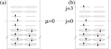
FIG. 2.: Two examples of states in the spin-$\frac{3}{2}$ sector of Hilbert space: (a) the ground state $|\frac{3}{2}\rangle$ and (b) the excited state $|\frac{3}{2},2\rangle$. The single-particle levels are drawn at $h=0$, and we indicated schematically how states are paired according to $(u_{i}+v_{i}c^{\dagger}_{i+}c^{\dagger}_{i-})$ in the BCS-like Ansätze (17) and (20) for $|\frac{3}{2}\rangle$ and $|\frac{3}{2},2\rangle$, with solid or dashed ellipses connecting states that would be completely filled or empty in the absence of pairing correlations.

FIG. 3.: Properties of spin-$s$ ground states $|s\rangle$ [compare Eq. (17)]: (a) The pairing parameters $\Delta_{s}(d)/\tilde{\Delta}$ for some spin-$s$ ground states $|s\rangle$, as a functions of $d/\tilde{\Delta}$. The critical level spacings $d_{c,s}$ at which $\Delta_{s}(d_{c,s})=0$ are found to be 2.36, 0.77, 0.44, 0.31, …for $s=0,1/2,1,3/2,\dots$, respectively. (b) The energy densities $({\cal E}_{s}-{\cal E}^{0}_{p/2})d/\tilde{\Delta}^{2}$ (solid lines), plotted as functions of $d/\tilde{\Delta}$ for $h=0$, of some pair-correlated spin-$s$ ground states $|s\rangle$ relative to the uncorrelated spin-$p/2$ Fermi sea $|p/2\rangle_{0}$, and for comparision the relative energy densities $({\cal E}^{0}_{s}-{\cal E}^{0}_{p/2})d/\tilde{\Delta}^{2}$ (dashed lines) of the corresponding uncorrelated paramagnetic states $|s\rangle_{0}$ (obtained from $|s\rangle$ by setting $\Delta_{s}=0$). We call the plotted quantities energy densities since the normalization factor $d/\tilde{\Delta}^{2}$ contains $d\sim\mbox{Vol}^{-1}$. The solid and dashed spin-$s$ lines meet at the critical level spacing $d_{c,s}$, above which no pairing correlations survive (so that the relative energy densities equal $(s^{2}-p/4+(s-p/2)\lambda)d^{2}/\tilde{\Delta}^{2}$ there).

FIG. 4.: Properties of excited spin-$\frac{1}{2}$ states $|\frac{1}{2},j\rangle$ [compare Eq. (20)]: (a) The pairing parameter $\Delta_{1/2,j}$ for some spin-$\frac{1}{2}$ states $|\frac{1}{2},j\rangle$ $(j=0,\dots,4)$, together with $\Delta_{0}$ of the spin-$0$ ground state $|0\rangle$ (the outermost curve). The larger $j$, the closer $\Delta_{1/2,j}$ approaches the spin-0 value $\Delta_{0}$. (b) The relative energy densities $({\cal E}_{1/2,j}-{\cal E}^{0}_{1/2,0})d/\tilde{\Delta}^{2}$ (solid lines) of $|\frac{1}{2},j\rangle$ relative to $|\frac{1}{2},0\rangle_{0}=|\frac{1}{2}\rangle_{0}$, and for comparison the relative energy densities $({\cal E}^{0}_{1/2,j}-{\cal E}^{0}_{1/2,0})d/\tilde{\Delta}^{2}$ (dashed lines) of the corresponding uncorrelated state $|\frac{1}{2},j\rangle_{0}$. For excited states the solid and dashed lines meet at a larger $d$ than for the ground state, i.e. in excited states pairing correlations survive down to smaller grain sizes than in the corresponding ground state.

FIG. 5.: The level-crossing fields $h_{s,s^{\prime}}(d)/\tilde{\Delta}$ [see Eq. (21)] for the cascade of ground state changes (GSCs) $(s_{0},s_{1})$; $(s_{1},s_{2})$; $\ldots$ that occurs as $h$ increases from 0 at given $d$. Some lines are labeled by the associated GSC $(s,s^{\prime})$ (where ${\cal E}_{s^{\prime}}$ drops below ${\cal E}_{s}$ as $h$ increases past $h_{s,s^{\prime}}$). (Level crossing fields not associated with a GSC are not shown.) The order in which GSCs can occur within a cascade (i.e. the order of $h_{s,s^{\prime}}$ lines encountered when moving vertically upward in the figure) depends sensitively on $d$, and an infinite number of distinct regimes (cascades) I, II, III, …can be distinguished.

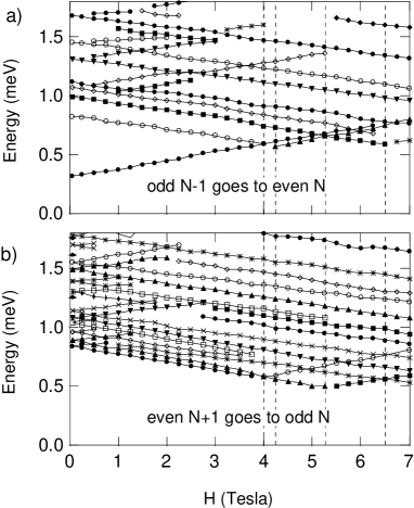
FIG. 6.: Experimental tunneling spectra measured by RBT (Fig. 3 of Ref. [9]). The distances between lines give the fixed-$N$ excitation spectra of (a) an even and (b) an odd grain, as explained in Section IV A. The vertical dashed lines indicate the first four level-crossing fields $H_{s,s^{\prime}}$ (assigned by comparison with Fig. 7, see Section IV B), namely $H_{0,1}\!=\!4$T, $H_{1/2,3/2}\!=\!4.25$T, $H_{1,2}\!=\!5.25$T and $H_{3/2,5/2}\!=\!6.5$T with uncertainty $\pm 0.13$T (half the $H$-resolution of 0.25T).

FIG. 7.: The theoretical odd-to-even and even-to-odd tunneling spectra $(\Delta E_{if}-\Delta E_{min}(0))/\tilde{\Delta}$ predicted for an ultrasmall superconducting grain as a function of magnetic field $h$, for two different level spacings: (a) $d=0.67\tilde{\Delta}$ and (b) $d=0.34\tilde{\Delta}$ (corresponding to regimes I and III of Fig. 5, respectively). Some lines are labeled by the corresponding $s_{i}\to s^{\prime}_{i}$ tunneling transition. Not all possible higher lines (corresponding to excited final states $|s,j\rangle$) are shown. Vertical dashed lines indicate those level-crossing fields $h_{s,s^{\prime}}$ [see Eq. (21] at which kinks or jumps occur, with $h_{0,1}<h_{1/2,3/2}<h_{1,2}<h_{3/2,5/2}$ in (a) and $h_{1/2,3/2}<h_{0,2}<h_{2,3}$ in (b).

FIG. 8.: The first jump in the lowest line of a tunneling spectrum occurs at the level-crossing field $h_{CC}(p,d)=h_{s_{0},s_{1}}$ that induces the first ground state change $(s_{0},s_{1})$. The size of this jump in units of $\tilde{\Delta}$, namely $|\Delta E_{s_{1},f^{\prime}}-\Delta E_{s_{0},f}|/\tilde{\Delta}$, is shown here as function of $d/\tilde{\Delta}$ for $e\to o$ (solid line) and $o\to e$ (dashed line) tunneling spectra. Both lines approach the CC value $1-1/\sqrt{2}=0.29$ as $d\to 0$. Their non-monotonic behavior is due to the discreteness of the level spacing; the kinks occur at the regime boundaries of Fig. 5, indicated here by vertical dashed lines.

FIG. 9.: Parity effect for the pair-breaking energies $\Omega_{e}\equiv\frac{1}{2}(E_{1}-E_{0})_{h=0}$ and $\Omega_{o}\equiv\frac{1}{2}(E_{3/2}-E_{1/2})_{h=0}$ (see Section IV C 2): when calculated naively using conventional mean-field theory (dashed lines), the pair-breaking energies obey $\Omega_{o}>\Omega_{e}$ for all $d/\tilde{\Delta}$; in contrast, when calculated within generalized variational BCS theory (solid lines), $\Omega_{o}<\Omega_{e}$ for $d/\tilde{\Delta}<0.6$; this reflects a parity effect, namely that $\Delta_{3/2}<\Delta_{1}$, which is caused by the extra unpaired electron in $|3/2\rangle$ relative to $|1\rangle$.

FIG. 10.: The parity parameter $\Delta_{P}^{\rm ML}$ discussed by Matveev and Larkin [14], calculated perturbatively for the uncorrelated Fermi sea ($\Delta_{P}^{\rm ML,pert}=\frac{1}{2}\lambda d$, dashed line), and using our generalized variational BCS-approach ($\Delta_{P}^{\rm ML,var}$ of Eq. (26), solid line). The renormalized result $\Delta_{P}^{\rm ML}$ of Eq. (28) given by ML is not shown since its range of validity is $d/\tilde{\Delta}\gg 1$.

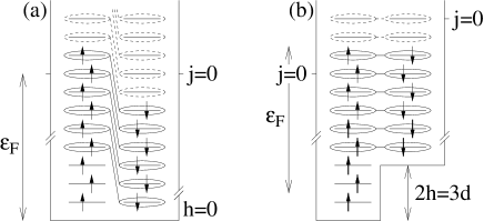
FIG. 11.: Schematic representations of the non-time-reversed-pairing state $|3/2\rangle^{\prime}$ defined in Eq. (30). The energies $\varepsilon_{j}\mp h$ of the single-particle states $|j,\pm\rangle$ are drawn (a) for $h=0$ and (b) for $2h=3d$. We indicated schematically how non-time-reversed states are paired according to $(u_{i}+v_{i}c^{\dagger}_{(i+3)+}c^{\dagger}_{i-})$ in the BCS-like Ansatz (30), with solid or dashed ellipses encircling states that would be completely filled or empty in the absence of pairing correlations.

FIG. 12.: $I$-$V$ characteristics for a SET with an ultrasmall superconducting grain as island (from Ref. [36]). The current is plotted as a function of gate charge ($Q_{g}/e$) and transport voltage ($eV/E_{C}$). Pairing correlations shift the degeneracy-point values of $Q_{g}/e$ away from their $e$-periodic values of $2m\pm\frac{1}{2}$ by $\pm E^{o/e}_{G}/E_{C}$ (see text). To better reveal the figure’s characteristic features, it was plotted using a ratio $E^{o/e}_{G}/E_{C}\simeq 0.1$, very much larger than the typical values of $<0.01$.

REFERENCES

- [1] A.W. Anderson, J. Phys. Chem. Solids 11, 28 (1959).
- [2] I. Giaver and H. R. Zeller, Phys. Rev. Lett. 20, 1504 (1968).
- [3] H. R. Zeller and I. Giaver, Phys. Rev. 181, 789 (1969).
- [4] M. Strongin, R. S. Thompson, O. F. Kammerer, and J. E. Crow, Phys. Rev. B 1, 1078 (1970).
- [5] B. Mühlschlegel, D.J. Scalapino, and R. Denton, Phys. Rev. B 6, 1767 (1972).
- [6] D. C. Ralph, C. T. Black, and M. Tinkham, Phys. Rev. Lett. 74, 3241 (1995).
- [7] C. T. Black, D. C. Ralph, and M. Tinkham, Phys. Rev. Lett. 76, 688 (1996).
- [8] D. C. Ralph, C. T. Black, and M. Tinkham, Physica (Amsterdam), 218B, 258 (1996).
- [9] D. C. Ralph, C. T. Black, and M. Tinkham, Phys. Rev. Lett. 78, 4087 (1997).
- [10] O. Agam, N. S. Wingreen, B. L. Altshuler, D. C. Ralph, and M. Tinkham, Phys. Rev. Lett. 78, 1956 (1997).
- [11] O. Agam and I. L. Aleiner, Phys. Rev. B 56, 5759 (1997).
- [12] J. von Delft, A. D. Zaikin, D. S. Golubev, and W. Tichy, Phys. Rev. Lett. 77, 3189 (1996).
- [13] R. A. Smith and V. Ambegaokar, Phys. Rev. Lett. 77, 4962 (1996).
- [14] K. A. Matveev and A. I. Larkin, Phys. Rev. Lett. 78, 3749 (1997).
- [15] F. Braun, J. von Delft, D. C. Ralph, and M. Tinkham, Phys. Rev. Lett. 79, 921 (1997).
- [16] S. Bahcall, unpublished.
- [17] B. Jankó, A. Smith, and V. Ambegaokar, Phys. Rev. B 50, 1152 (1994).
- [18] D. S. Golubev and A. D.Zaikin, Phys. Lett. A 195, 380 (1994); Qantum Dynamics of Submicron Structures, H. A. Cerdeira et al. (Eds.) Kluwer Acad. Publ., 473 (1995).
- [19] V. G. Soloviev, Mat. Fys. Skrif. Kong. Dan. Vid. Selsk. 1, 1 (1961).
- [20] Ya. M. Blanter, private communication (1996).
- [21] R. Meservey and P. M. Tedrow, Phys. Rep. 238, 173 (1994).
- [22] P. Ring and P. Schuck, The Nuclear Many-Body Problem, Springer-Verlag, (1980).
- [23] L. N. Cooper, J. Bardeen, and J. R. Schrieffer, Phys. Rev. 108, 1175 (1957).
- [24] D. C. Ralph. Private communication.
- [25] F. Braun, and J. von Delft, to be published.
- [26] R. Balain, H. Flocard, and M. Veneroni, nucl-th/9706041 (1997).
- [27] A. Mastellone, G. Falci, and R. Fazio, unpublished (1997).
- [28] J. W. Garland, K. H. Bennemann, and F. M. Mueller, Phys. Rev. Lett. 21, 1315 (1968).
- [29] R. Meservey, P. M. Tedrow, and Peter Fulde, Phys. Rev. Lett. 25, 1270 (1970).
- [30] B. S. Chandrasekhar, Appl. Phys. Lett. 1, 7 (1962).
- [31] A. M. Clogston, Phys. Rev. Lett. 9, 266 (1962).
- [32] M. T. Tuominen, J. M. Hergenrother, T. S. Tighe, and M. Tinkham, Phys. Rev. Lett. 69, 1997 (1992); Phys. Rev. B 47, 11599 (1993); M. Tinkham, J. M. Hergenrother, and J. G. Lu, Phys. Rev. B 51, 12649 (1996).
- [33] P. Lafarge, P. Joyez, D. Esteve, C. Urbina, and M.H. Devoret, Phys. Rev. Lett. 70, 994 (1993).
- [34] D. L. Klein, R. Roth, A. K. L. Lim, A. P. Alivisatos and Paul L. McEuen, Nature 389, 699 (1997).
- [35] Boris L. Altshuler, private communication (1997).
- [36] Wolfgang Tichy, Diploma thesis, University Karlsruhe (1996).