Magnetization switching in a Heisenberg model for small ferromagnetic particles

Abstract

We investigate the thermally activated magnetization switching of small ferromagnetic particles driven by an external magnetic field. For low uniaxial anisotropy the spins can be expected to rotate coherently, while for sufficient large anisotropy they should behave Ising-like, i. e. , the switching should then be due to nucleation. We study this crossover from coherent rotation to nucleation for the classical three-dimensional Heisenberg model with a finite anisotropy. The crossover is influenced by the size of the particle, the strength of the driving magnetic field, and the anisotropy. We discuss the relevant energy barriers which have to be overcome during the switching, and find theoretical arguments which yield the energetically favorable reversal mechanisms for given values of the quantities above. The results are confirmed by Monte Carlo simulations of Heisenberg and Ising models.

Pacs: 75.10.Hk, 75.40.Mg, 64.60.Qb

I Introduction

The size of magnetic particles plays a crucial role for the density of information storage in magnetic recording media. Sufficiently small particles become single-domain particles, which improves their quality for magnetic recording. On the other hand, when the particles are too small they become superparamagnetic and no information can be stored (see e. g. [1] for a review). Hence, much effort has recently been focused on the understanding of small magnetic particles, especially since recent experimental techniques allow for the investigation of isolated single-domain particles [2, 3, 4, 5].

In this paper focus is on the reversal of ferromagnetic particles of finite size. We investigate the influence of the size and anisotropy of the particle on the possible reversal mechanisms, two extreme cases of which are coherent rotation and nucleation. The latter mechanism has been a subject of common interest in recent years [6, 7, 8, 9, 10, 11], studied mainly theoretically in Ising models, which can be interpreted as a classical Heisenberg model in the limit of infinite anisotropy. It is the aim of this paper to study the crossover from magnetization reversal due to nucleation for high anisotropy to coherent rotation [12, 13] for lower anisotropy.

Throughout the paper we will consider a finite, spherical three- dimensional system of magnetic moments. These magnetic moments may represent atomic spins or block spins following from a coarse graining of the physical lattice [14]. Our system is defined by a classical Heisenberg Hamiltonian,

$${\cal H}=-J\sum_{\langle ij\rangle}{\bf S}_{i}\cdot{\bf S}_{j}-d\sum_{i}(S^{z}_{i})^{2}-{\bf B}\cdot\sum_{i}{\bf S}_{i}.$$ (1)

where the ${\bf S}_{i}$ are three-dimensional vectors of unit length. The first sum which represents the exchange of the spins, is over nearest neighbors with the exchange coupling constant $J$. The second sum represents an uniaxial anisotropy which favors the $z$-axis as easy axis of the system (anisotropy constant $d>0$). The last sum is the coupling of the spins to an applied magnetic field, where ${\bf B}$ is the strength of the field times the absolute value of the magnetic moment of the spin. We neglect dipolar interaction. Although in principle it is possible to consider dipolar interaction in a Monte Carlo simulation [14] this needs much more computational effort due to the long range of the dipolar interaction and, hence, exceeds current computer capacities . Therefore, the validity of our results is restricted to particles which are small enough to be single-domain in the remanent state [15].

In the following, we will investigate the thermally activated reversal of a particle which is destabilized by an magnetic field pointing in a direction antiparallel to the initial magnetization which is parallel to the easy axis of the system. Due to the finite temperature and the magnetic field, after some time the particle will reverse its magnetization, i. e. the $z$-component of the magnetization will change its sign.

In section II, we determine the energy barriers which have to be overcome by thermal fluctuations for the two cases of coherent rotation and nucleation within a classical theory. By a comparison of the energy barriers, we derive where the crossover from one mechanism to the other occurs.

In section III we compare our theoretical considerations with numerical results from Monte Carlo simulations of Heisenberg and Ising models, and we relate the lifetime of the metastable state to the theoretical energy barriers for the different reversal mechanisms.

II Theory

A Coherent rotation

We give here a brief summary of the results of the theory of Néel [12] and Brown [13], since we need this concept for the further progress of our theoretical considerations.

Let us consider a spherical, homogeneously magnetized particle of radius $R$. The simplest theoretical description for the reversal of such a particle is to assume that the reversal mechanism is coherent rotation, i. e. a uniform rotation of all spins of the particle. This reversal process can be described by an angle of rotation $\theta$ between the easy axis of the system – which in our case will be antiparallel to the direction of the magnetic field – and the magnetization of the particle. The increase of the energy during the reversal is then

$$\Delta E=-dV\cos^{2}{\theta}-BMV\cos{\theta}.$$ (2)

Since this equation should be comparable to Eq. 1, the anisotropy constant $d$ is an anisotropy energy per unit cell (spin), and $V=(4/3)\pi R^{3}$ is the volume of the particle as a number of unit cells. $B$ is - as before - the absolute value of the applied field times the magnetic moment of a unit cell and, hence, $M$ the spontaneous magnetization per magnetic moment. The energy barrier which has to be overcome is due to the anisotropy of the system. It is the maximum of $\Delta E$ with respect to $\theta$:

$$\Delta E_{cr}=\frac{4\pi R^{3}d}{3}-{\frac{4\pi R^{3}BM}{3}}+\frac{\pi R^{3}B^{2}M^{2}}{3d}$$ (3)

The corresponding lifetime of the metastable state is then

$$\tau\sim\exp\left(\frac{\Delta E_{cr}}{T}\right)$$ (4)

for temperature $T\ll\Delta E_{cr}$. The two equations above are physically relevant only for

$$d>MB/2.$$ (5)

Otherwise there is no (positive) energy barrier, and hence the reversal is spontaneous without the need for thermal activation. This is the region of nonthermal reversal.

B Nucleation

For a system with a sufficient large anisotropy, it might be energetically favorable to divide into parts with opposite directions of magnetization parallel to the easy axis in order to minimize the anisotropy energy barrier. This kind of reversal mechanism is called nucleation [16] (see [8] for a recent review). The simplest case of a reversal process driven by nucleation for a system of finite size is the growth of one single droplet starting at one point of the boundary of the system (see also [11] for a corresponding calculation for a two-dimensional system). Due to the growth of the droplet a domain wall will cross the system, and the energy barrier which has to be overcome is caused by the domain-wall energy. We assume that the domain wall will have a curvature defined by a radius $r$ (see Fig. 1).

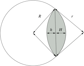
FIG. 1.: The nucleation of a droplet at the boundary of a spherical particle.

Then the surface of the domain wall is $F=2\pi rh$ and the volume of the droplet (the shaded region in Fig. 1) is $V_{d}=\pi H^{2}(3R-H)/3+\pi h^{2}(3r-h)/3$. The energy increase during the reversal of the particle is

$$\Delta E=2\sigma F-2MBV_{d},$$ (6)

where $\sigma$ is the energy density of the domain wall. Furthermore, it is $h=r-\sqrt{r^{2}-2HR+H^{2}}$, since the quantities in Fig.1 are not independent. Hence the energy increase can be expressed in terms of $H$, which is a measure for the penetration depth of the domain wall and its curvature $r$. These two quantities define the geometry of the droplet. Next we determine that curvature $r_{\mbox{min}}$ which minimizes the energy increase by the condition $\frac{\partial{\Delta E}}{\partial{r}}=0$, yielding the physically relevant solution

$$r_{\mbox{min}}=\frac{2\sigma}{MB}$$ (7)

which is also the radius of a critical droplet for classical nucleation in a bulk material.

The energy barrier $\Delta E_{w}$ which has to be overcome during the reversal is the maximum of the energy increase with respect to $H$. From the condition $\frac{\partial{\Delta E}}{\partial{H}}=0$, the physically relevant solution

$$H_{\mbox{max}}=R\Big{(}1-\frac{x}{\sqrt{x^{2}+4}}\Big{)}$$ (8)

follows with $x=MBR/\sigma$. Inserting the two conditions above into the formula for the energy increase yields the energy barrier for nucleation

$$\Delta E_{n} = \frac{4\pi R^{2}\sigma}{3x^{2}\sqrt{x^{2}+4}}\Big{(}x^{4}+(4-x^{3})\sqrt{x^{2}+4}+2x^{2}-8\Big{)}$$ (9)

This expression has two important limits. The first is the limit of infinite system size,

$$\lim_{R\rightarrow\infty}\Delta E_{n}=\frac{16\pi\sigma^{3}}{3M^{2}B^{2}},$$ (11)

where we obtain half of the energy barrier of the classical nucleation theory for a bulk system. The reduction by a factor of $\frac{1}{2}$ is due to the fact that for open boundary conditions only one-half of a critical droplet has to enter the system from the boundary.

The other interesting limit is that of small magnetic fields, where Eq.LABEL:e:edw can be expanded with respect to $x=MBR/\sigma$ resulting in

$$\Delta E_{n}\approx 2\pi R^{2}\sigma-\frac{4\pi BR^{3}M}{3}+\frac{3\pi B^{2}R^{4}M^{2}}{8\sigma}+\ldots$$ (12)

This means that for a small field $B$ the energy barrier of a nucleation process is the energy of a flat domain wall in the center of the particle plus corrections which start linearly in $B$. In contrast to the Néel-Brown theory, here, for vanishing magnetic field, the energy barrier is proportional to the cross-sectional area of the particle rather than its volume (see also the work of Braun [17]), which consequently reduces the coercivity of the particle.

C Comparison of coherent rotation and nucleation

Comparing the two energy barriers for coherent rotation (Eq.3) and nucleation (Eq.LABEL:e:edw), we can evaluate which reversal mechanism has the lower activation energy for a given set of values of $R$, $B$, $\sigma$, and $d$. A corresponding diagram is shown in Fig. 2 for a system of radius $R=4$ spins, where we set $M=1/$spin and $\sigma=J/\mbox{spin}$.

FIG. 2.: Diagram showing the regions of different reversal mechanisms for a particle of size $R=4$ spins, with $\sigma=J/$spin and $M=1/$spin. The points are results from Monte Carlo simulations (see Section III).

For large anisotropy the reversal is dominated by nucleation – the particle behaves like an Ising system. The crossover line $d_{c}(B,\sigma,R)$ which separates the region of reversal by nucleation from the region of coherent rotation can be determined by the condition that here the energy barriers for a nucleation process and for coherent rotation are equal. This condition results in

$$d_{c} = \frac{\sigma}{R}\Big{(}\frac{2}{x^{2}}+\frac{1}{\sqrt{x^{2}+4}}\big{(}1-\frac{4}{x^{2}}+\frac{x^{2}}{2}\big{)}$$ (14)

$$+\frac{1}{x^{2}}\sqrt{-3x^{2}+8+(2x^{2}-4)\sqrt{x^{2}+4}}\Big{)}.$$

For vanishing magnetic field, the formula above has a finite limit,

$$\lim_{B\rightarrow 0}(d_{c})=\frac{3\sigma}{2R}.$$ (15)

For large particle size, Eq. 14 has the simple asymptotic form

$$\lim_{R\rightarrow\infty}(d_{c})=\frac{BM}{2}$$ (16)

which, interestingly, is also the limit for nonthermal reversal (see Eq. 5). This means that for increasing particle size the region where a thermally activated reversal by coherent rotation occurs vanishes. For an infinite particle size the reversal is always either nonthermal or it is driven by nucleation – depending only on the ratio of the magnetic field to the anisotropy.

All the considerations above can be expected to be relevant only for sufficiently low temperatures. For higher temperatures the situation is more complicated. That is, for the nucleation regime, a crossover from single-droplet to multi-droplet nucleation – with different energy barriers) – is discussed in the literature (see [18, 19, 20] and references therein).

Apart from that, in a system with a given finite anisotropy the domain walls may be extended to a certain domain wall width $\xi$. For large anisotropy $\xi$ becomes as small as one lattice constant. This is the Ising case, where the domain-wall energy density is $\sigma\approx J/$spin. For smaller anisotropy the domain walls become more extended, and $\sigma$ decreases. Hence the crossover from nucleation to coherent rotation may be softened by the occurrence of extended domain walls. In this sense, pure coherent rotation could also be interpreted as a domain-wall-driven reversal, where the width of the domain wall is larger than the particle size. Obviously, our theoretical considerations discuss only two extreme cases. How realistic they are has to be tested numerically.

III Monte Carlo Simulation

A Method

Due to the many degrees of freedom of a spin system, numerical methods have to be used for a detailed microscopic description of the system. Since we are especially interested in the thermal properties of the system, we use Monte Carlo methods [21] for the simulation of the magnetic particle. Although a direct mapping of the time scale of a Monte Carlo simulation on experimental time scales is not possible, this method provides information on the dynamical behavior of the system since it solves the master equation for the irreversible behavior of the system [22].

We consider spins on a simple cubic lattice of size $L\times L\times L$, and simulate spherical particles with radius $R=L/2$ and open boundary conditions on this lattice.

One single spin flip of our Monte Carlo procedure consists of three parts. First, a spin is chosen randomly and a trial step is made (the role of which we will discuss below). Second, the change of the energy of the system is computed according Eq. 1. Third, the trial step is accepted with the probability from the heat-bath algorithm. Let us call one sweep through the lattice and performing the procedure explained above once per spin one Monte Carlo step (MCS).

Since we are interested in different reversal mechanisms, we designed a special algorithm which can simulate all of them efficiently. We use three different kinds of trial steps: First, a trial step in any spin direction uniformly distributed in spin space. This step does not depend on the initial direction of the spin. It samples the whole phase space efficiently and guarantees ergodicity. Second, a small step within a limited circular region around the initial spin direction. This step can efficiently simulate the coherent rotation. Third, a reflection of the spin. This step guarantees that, in the limit of large anisotropy, our algorithm crosses over to an efficient simulation of an Ising-like system. For each Monte Carlo step we use one of these different trial steps. Our algorithm then consists of a series of Monte Carlo steps using the different trial steps above. Altogether, our algorithm is ergodic, and it guarantees that all possible reversal mechanisms may occur in the system and can be simulated efficiently. As we tested by comparing simulations with different combinations of trial steps, and as we will demonstrate in the section III B, for a two-spins system, this algorithm does not artificially change our results.

Simulations of Heisenberg systems are much more time consuming, than e. g. , those of Ising systems, since the Heisenberg system has many more degrees of freedom. Apart from that, to obtain results which are comparable to our theoretical considerations we have to perform simulations in the limit of low temperatures, $T\ll T_{c}$, where the critical temperature $T_{c}$ is 1.44$J$ for anisotropy $d=0$ [23]. Here, the metastable lifetimes are long – for single runs up to $5\times 10^{7}$MCS in our simulation. Therefore, for the Heisenberg system we had to restrict ourselves to rather small system sizes, $L=4,8,12$. However, we tried to minimize the statistical error by performing an average over many Monte Carlo runs ($100\ldots 1000$). Since the theoretical considerations which we want to proof are for finite system sizes, and since, hence, the radius of the particle is a variable of the theory we belive that the rather small system sizes of the simulation are no disadvantage. Apart from that, for comparison we also performed Monte Carlo simulations of an Ising model where we also used larger system sizes of up to $L=28$.

The simulations were performed on an IBM-RS6000 workstation cluster and on two Parsytec CC parallel computers (8 and 24 PPC604 nodes, respectively).

B Results for the Heisenberg system

We start our simulation with an initial spin configuration where all spins are pointing up (all spins ${\bf S}_{i}=(0,0,1)$). The magnetic field ${\bf B}=(0,0,-B)$ destabilizes the system, and after some time the magnetization of the system will reverse. The metastable lifetime $\tau$ is defined by the condition $M_{z}(\tau)=0$ where $M_{z}$ is the $z$-component of the magnetization ${\bf M}=(1/N)\sum_{i}{\bf S}_{i}$.

FIG. 3.: Metastable lifetime $\tau$ vs. $1/T$ for a system of two spins. $B=0.5J$. Two different anisotropies, $d=1.5$/spin (nucleation) and $d=0.5J$/spin (coherent rotation). The solid lines correspond to Eq. 4, with the energy barriers explained in the text.

First, we tested our algorithm by simulating the simplest imaginable system that can show both coherent rotation and nucleation – a two-spin system. Here the energy barrier is $\Delta E_{n}=2(J-B)$ for nucleation (i. e. , the spins are antiparallel during the reversal) and $\Delta E_{cr}=2d(1-B/(2d))^{2}$ for coherent rotation (i. e. , the spins are always parallel during the reversal). For low temperatures we expect a behavior following thermal activation as in Eq. 4 with the energy barriers above. Figure 3 demonstrates that in the limit of low temperatures, we actually obtain constant slopes for the $\ln\tau$ vs. $1/T$ data, and the slopes agree perfectly with the theoretical energy barriers above. Hence our simulation is in agreement with the theoretical expectations.

Now we turn to the simulation of larger systems.

FIG. 4.: Snapshots of simulated spin configurations at the lifetime $\tau$. Shown is one central plane of systems of size $R=6$ spins. $B=0.7J$. a) Coherent rotation ($d=0.35J$/spin, $T=0.09J$). b) Nucleation ($d=0.7J$/spin, $T=0.45J$).

Fig. 4 shows spin configurations of simulated systems of size $R=6$ spins at the metastable lifetime $\tau$. For simplicity, only one central plane of the three-dimensional system is shown. The $z$-axis of the spin components is pointing up. For sufficient low anisotropy (Fig.4a) the spins rotate nearly coherently. At the metastable lifetime $\tau$ the magnetization vector of the system points to any given direction in the $x-y$-plane. Therefore, as horizontal component of the spins we show here that component of the $x-y$-plane of the spin space that has the largest

FIG. 5.: $M$, $M_{\perp}$, and $M_{z}$ of one $R=6$ spins - system as in Fig.4: $B=0.7J$. a) Coherent rotation ($d=0.35J$/spin, $T=0.09J$). b) Nucleation ($d=0.7J$/spin), $T=0.45J$.

contribution. For larger anisotropy (Fig.4b) the reversal is driven by nucleation. Since it is $M_{z}(\tau)=0$, the domain wall at that time is in the center of the system dividing the particle into two oppositely magnetized parts of equal size.

Fig. 5 shows the corresponding time dependence of the $z$-component of the magnetization, its absolute value $M=|{\bf M}|$, and its planar component $M_{\perp}=\sqrt{M_{x}^{2}+M_{y}^{2}}$ for the same simulation from which the spin configurations of Fig.4 stem. For the case of coherent rotation there is a continuous growth of the planar component of the magnetization during the reversal, while the absolute value of the magnetization remains nearly constant – apart from a small dip at the lifetime $\tau\approx 19000$MCS. For the case of nucleation the planar component of the magnetization is nearly constant zero except of a small hump at the lifetime $\tau\approx 34000$MCS. Here the absolute value of the magnetization breaks down.

These results lead us to the following approach to characterize the reversal mechanisms numerically: we determine the absolute value of the magnetization at the lifetime, $M(\tau)$. In order to obtain reasonable results we have to take an average over many runs, so that we define a quantity $\mu=[M(\tau)]$ where the square brackets denote an average over many Monte Carlo runs (or systems). This quantity should go to zero for a nucleation-driven reversal, and should be finite for coherent rotation. The maximum value of $\mu$ in the limit of low anisotropy should be the spontaneous magnetization.

In order to confirm our theoretical results numerically, we simulated $\mu$ for different values of the anisotropy $d=0.2\ldots 2J/$spin, the magnetic field $B=0.7\ldots 1.2J$, and the system size $R=2\ldots 6$ spins. We took an average over 100 ($R=6$) to 1000 ($R=2$) runs. Fig. 6 shows the results for the anisotropy dependence of $\mu$ for different system sizes and the lowest temperatures that have been simulated ($T=0.71\ldots 0.04J$ depending on $d$). The influence of the temperature on the simulations will be discussed later in connection with Fig. 8.

FIG. 6.: $\mu$ vs. anisotropy for different system sizes. $B=0.7J$, $T=0.71\ldots 0.04J$ depending on $d$.

As expected, for small anisotropy, $\mu$ tends to a finite limit while with increasing anisotropy the curves converge to zero. This effect is stronger the larger the system size is — a behavior that appears to be analogous to the finite size behavior of a system undergoing a phase transition. The corresponding finite-size scaling ansatz [21] is

$$\mu=R^{-\beta/\nu}\tilde{\mu}^{\pm}\left(|d_{\infty}-d|R^{1/\nu}\right)$$ (17)

where the scaling function $\tilde{\mu}^{\pm}\sim x^{\beta}$ for $x\rightarrow\infty$ so that

FIG. 7.: Scaling plot of $\mu$ vs. anisotropy for different system sizes. Data correspond to Fig. 6

in the limit of infinite system size it is $\mu\sim(d_{\infty}-d)^{\beta}$ for $d<d_{\infty}$. In order to test if this scaling form can be applied to the data shown in Fig. 6, we present a corresponding scaling plot in Fig. 7. The data collapse rather well, using $d_{\infty}=B/2=0.35J/\mbox{spin}$, $\beta/\nu=0.5\pm 0.1$, and $1/\nu=0.9\pm 0.1$.

Obviously, in the limit $R\rightarrow\infty$ $\mu(d)$ behaves like an order parameter at a second-order phase transition: it is zero for $d>d_{\infty}$ and finite for $d<d_{\infty}$, following $\mu\sim(d_{\infty}-d)^{\beta}$.

The fact that for infinite system size the transition occurs at $d_{\infty}=B/2$ is in agreement with our theoretical considerations, since for $R\rightarrow\infty$ the region of thermally activated coherent rotation vanishes and the crossover from nucleation to (nonthermal) coherent rotation occurs at $d_{c}(R\rightarrow\infty)=B/2$ (Eq. 16). That is, only for $d<B/2$ will the particle rotate coherently, and $\mu$ must be finite. However, to what degree the crossover from nucleation to coherent rotation for infinite system size may be described as a phase transition must be left for future research.

In the following we will restrict ourselves on systems of finite size. In order to differentiate numerically between the two reversal mechanisms for systems of finite size, we use a criterion that also comes from a study of phase transitions: we define the inflection point of the curves $d(B)$ as that value $d_{c}(B,R)$ where the crossover from nucleation to coherent rotation occurs. These points are shown in Fig. 2. For large $B$ they agree very well with the theoretical line. For lower $B$ the numerical values are slightly too small. This systematic deviation might be due to the fact that the theoretical energy barrier for nucleation is overestimated assuming $\sigma=J/$spin: due to occurrence of extended domain walls for lower anisotropy the domain wall energy might be reduced. This also reduces the energy barrier of the nucleation process and consequently, here crossover to nucleation occurs earlier.

Apart from the numerical determination of the cross overline $d_{c}$ discussed above, we also tried to compute the relevant energy barriers directly. During the simulation, temperature plays a crucial role. The larger $d$ is, the larger is the energy barrier which has to be overcome by thermal activation and, hence, the higher the temperature has to be during the simulation in order to obtain results within a given computing time. On the other hand, we have to simulate as low temperatures as possible to see the behavior that is described by our theoretical considerations. Therefore, varying the anisotropy, we have to adjust the temperature. Fig. 8 shows the temperature dependence of the metastable lifetime for different anisotropies. To save computer time, instead of an average of the lifetimes of the individual Monte Carlo runs, we calculated the median [6]. In the limit of low temperature we expect a behavior following thermal activation as in Eq. 4, with the energy barrier following from the theoretical consideration in section II.

FIG. 8.: Metastable lifetime $\tau$ vs. $1/T$ for four different anisotropies. System size $R=4$ spins and $B=1J$.

As Fig. 8 shows, this dependence (i. e. , constant slopes in Fig. 8 for low $T$) can hardly be observed. All curves have a finite curvature even for the lowest simulated temperature except of that for $d=0.4J$/spin, where the energy barrier is zero. We conclude that we could not reach low enough temperatures within the simulations and, hence, we analyse our data in the following way: We take the local slope of $(\ln\tau)(1/T)$ as temperature-dependent energy barrier. These energy barriers versus $d$ are shown in Fig. 9 for three different temperatures, and they are compared with the theoretical results. The magnetic field is $B=1J$. Hence, for $d<0.5J/$spin – the nonthermal region (Eq. 16) – it is $\Delta E=0$. In the regime for thermally activated coherent rotation, i. e. , between $d<0.5J/$spin and the crossover anisotropy $d_{c}$ (Eq. 14), the energy barrier increases following Eq. 3. Above $d_{c}$ which is roughly $0.65J/$spin, here the energy barrier remains constant since in the nucleation regime it does not depend on $d$ (Eq. LABEL:e:edw).

FIG. 9.: Comparison of the theoretical curve for the $d$-dependence of the energy barrier with the numerical data for different temperatures following from Fig. 8.

Comparing our numerical results with this theoretical curve, we find agreement as far as the crossover from nonthermal reversal to thermally driven coherent rotation is concerned. Also, we observe that in principal the numerical results seem to converge with decreasing temperature. However, within these simulation we cannot confirm the theoretical curve very accurately, especially the asymptotic behavior of the nucleation regime. We conclude that the main reason for this quantitative deviation is that we do not obtain the asymptotic low-temperature energy barriers, since these depend still on the temperature.

One additional reason for deviations in the coherent rotation regime might be that, in order to compare the results of our simulation with the theoretical results, we had to estimate the domain-wall energy density $\sigma$, which here we simply set to $\sigma=J/$spin. This estimate might be to large for a Heisenberg system which can develop extended domain walls with a lower domain-wall energy. We could try to fit $\sigma$ in such a way that it we obtain a reasonable agreement with the numerical data, but this would not solve the problem mentioned above, namely, that we are not in the asymptotic low-temperature regime.

C Results for the Ising system

In order to confirm our theoretical results for the energy barrier of the nucleation regime, it is much more straightforward to simulate an Ising system directly instead of a Heisenberg system with large anisotropy. Therefore, we performed a standard Monte Carlo simulation of an Ising system defined by the Hamiltonian

$${\cal H}=-J\sum_{\langle ij\rangle}S_{i}S_{j}-B\sum_{i}S_{i}$$ (18)

with $S_{i}=\pm 1$. As before, we simulated spherical particles with radius $r=L/2$ on a simple cubic lattice of size $L\times L\times L$ with open boundary conditions. For the Ising system, $L$ was varied from $L=4$ to $L=32$. We used the same methods as above, performing averages over 50-100 Monte Carlo runs depending on the system size.

Fig. 10 shows the resulting temperature dependence of the metastable lifetime. In our data for the Ising system, a thermal activation corresponding to Eq.4 can be much better extracted than for the Heisenberg system. For low enough temperatures, straight lines can be fitted to the data the slope of which determine the activation barrier $\Delta E_{n}$.

FIG. 10.: Metastable lifetime $\tau$ vs. $1/T$ for two different magnetic fields. System size $R=4$ spins.

For a comparison of our numerically determined activation barriers with Eq.LABEL:e:edw for the theoretical energy barriers of the nucleation process, once more we have to estimate the domain-wall energy density $\sigma$. In an Ising system, the domain-wall width is reduced to one lattice constant and, hence, the domain-wall energy cannot be reduced by an extended width of the wall. But, on the other hand, on a cubic lattice the energy of a domain wall per spin depends on the direction of the domain wall with respect to the axis of the lattice. This is $J/$spin for a wall parallel to the axis but, larger for walls in diagonal directions. Thus, we can expect $\sigma$ to be little larger than $J/$spin, and in the following it is set to $\sigma=1.2J$.

FIG. 11.: Comparison of the theoretical curve for the energy barrier (Eq. LABEL:e:edw) with the numerical data for different system sizes and $B=0.1\ldots 0.8$. $x=MBR/\sigma$.

Fig. 11 compares our numerical data with Eq. LABEL:e:edw. Since $\Delta E_{n}/(R^{2}\sigma)$ depends only on the variable $x=MBR/\sigma$, the data for different system sizes collapse on one single curve, and the agreement of our numerical data with the theoretical curve is satisfactory.

IV Conclusions

We investigate the magnetization reversal of a classical Heisenberg system for single-domain ferromagnetic particles. Varying the anisotropy one expects different reversal mechanisms, the extreme cases of which are coherent rotation and nucleation, which in the case of a single-droplet-nucleation is a reversal by domain-wall motion. We studied the crossover from switching due to nucleation for high anisotropy, high fields, and large systems to coherent rotation for lower anisotropy, lower fields, and smaller systems. By a comparison of the relevant energy barriers, we derive a formula which estimates where the crossover from the one mechanism to the other occurs.

If we insert the material parameters for CoPt [14], $\sigma=0.004\mbox{J/m}^{2}$, and $d=200$kJ/$\mbox{m}^{3}$ in Eq. 15, we find that for vanishing magnetic field a reversal by nucleation should occur for particles with a radius larger than 15nm. While at the moment we are not aware of any direct measurement of this crossover, experimental hints of the occurrence of different, particle-size-dependent reversal mechanism were published by Wernsdorfer et al. [4].

As one important result, we found that in the limit of large particle size the region where a thermally activated coherent rotation occurs vanishes. This means that for large particles the rotation is always either nonthermal or driven by nucleation, depending only on the ratio of the driving field to the anisotropy. Second, in the nucleation regime the energy barrier is reduced, since here – in contrast to the Néel-Brown theory – for vanishing magnetic field the energy barrier is proportional to the cross-sectional area of the particle rather than its volume.

We confirmed the result above by simulations. We also tried to determine the relevant energy barriers numerically. For the case of the Heisenberg model we could hardly reach the low-temperatures limit which one needs in order to see the simplest, lowest-energy reversal mechanism. However, for an Ising model, i. e. , in the limit of infinite anisotropy we could establish our formulas for the energy barrier of a single-droplet nucleation process.

Acknowledgments: We thank K. D. Usadel for helpful suggestions and critically reading of the manuscript. The work was supported by the Deutsche Forschungsgemeinschaft through Sonderforschungsbereich 166 and through the Graduiertenkolleg ”Heterogene Systeme”.

REFERENCES

- [1] R. W. Chantrell and K. O’Grady, in Applied Magnetism, edited by R. Gerber, C. D. Wright, and G. Asti (Kluwer Academic Publishers, Dordrecht, 1994), p. 113
- [2] C. Salling, R. O’Barr, S. Schultz, I. McFadyen, and M. Ozaki. J. Appl. Phys. 75, 7986 (1994)
- [3] M. Lederman, S. Schultz, and M. Ozaki, Phys. Rev. Lett. 73, 1986 (1994)
- [4] W. Wernsdorfer, K. Hasselbach, D. Mailly, B. Barbara, A. Benoit, L. Thomas, and G. Suran, J. Mag. Mag. Mat. 140, 389 (1995)
- [5] W. Wernsdorfer, E. Bonet Orozco, K. Hasselbach, A. Benoit, B. Barbara, N. Demoncy, A. Loiseau, H. Pascard, and D. Mailly, Phys. Rev. Lett. 78, 1791 (1997)
- [6] D. Stauffer, Int. J. Mod. Phys. C 3, No.5, 1059 (1992)
- [7] H. Tomita and S. Miyashita, Phys. Rev. B 46, 8886 (1992).
- [8] P. A. Rikvold and B. M. Gorman, in Annual Reviews of Computational Physics I, edited by D. Staufer (World Scientific, Singapore, 1994), p. 149
- [9] M. Acharyya and B. Chakrabarti, Phys. Rev. B 52, 6550 (1995)
- [10] D. García-Pablos, P. García-Mochales, N. García, and P. A. Serena, J. Appl. Phys. 79, 6019 (1996)
- [11] H. L. Richards, M. Kolesik, P. A. Lindgård, P. A. Rikvold, and M. A. Novotny, Phys. Rev. B 55, 11521 (1997)
- [12] L. Néel, Ann. Geophys. 5, 99 (1949)
- [13] W. F. Brown, Phys. Rev. 130, 1677 (1963)
- [14] U. Nowak, J. Heimel, T. Kleinefeld, and D. Weller, Phys. Rev. B 56, 8143 (1997)
- [15] A. Aharoni, J. Appl. Phys. 63, 5879 (1988)
- [16] R. Becker and W. Döring, Ann. Phys. (Leipzig) 24, 719 (1935)
- [17] H. B. Braun, Phys. Rev. Lett. 71, 3557 (1993)
- [18] K. Binder and H. Müller-Krumbhaar, Phys. Rev. B 9, 2328 (1974)
- [19] T. S. Ray and J. -S. Wang, Physika A 167, 580 (1990)
- [20] H. L. Richards, S. W, Sides, M. A. Novotny, and P. A. Rikvold, J. Mag. Mag. Mat. 150, 37 (1995)
- [21] K. Binder and D. W. Heermann, Monte Carlo Simulation in Statistical Physics (Springer-Verlag, Berlin, 1988), p. 21
- [22] F. Reif, Fundamentals of statistical and thermal physics (McGraw-Hill Book Company, New York 1965), p. 548
- [23] R. G. Brown and M. Ciftan, Phys. Rev. Lett. 76, 1352 (1996)