Gas of self-avoiding loops on the brickwork lattice

Abstract

An exact calculation of the phase diagram for a loop gas model on the brickwork lattice is presented. The model includes a bending energy. In the dense limit, where all the lattice sites are occupied, a phase transition occuring at an asymmetric Lifshitz tricritical point is observed as the temperature associated with the bending energy is varied. Various critical exponents are calculated. At lower densities, two lines of transitions (in the Ising universality class) are observed, terminated by a tricritical point, where there is a change in the modulation of the correlation function. To each tricritical point an associated disorder line is found.

Submitted for publication to: Saclay, SPhT/97-xxx
“Journal of Physics A”
PACS: 05.50.+q, 64.60.Kw

I Introduction

Models of closed loops on lattices in two dimensions have attracted considerable attention [1]. In a theoretical context they arise naturally as high-temperature expansions of spin models and they are closely related to integrable systems such as vertex models [2]. Loops on a lattice may also be regarded as simple models for (short) ring polymers in solution [3, 4]. The segments of the loop are then regarded as monomers, or small clusters of monomers. While realistic systems are three-dimensional, the two-dimensional case provides rich critical behaviour, and it may be hoped that some features hold in higher dimensions. Solid-on-solid models used in the study of roughening transitions in three-dimensional growth may also be mapped onto various two-dimensional loop-gas models [1].

In this paper a model of loops is studied, consisting of self-avoiding rings with a bending energy. We are mainly interested in the effects of varying the density of monomers on the lattice and the temperature. The model is defined as follows. Each bond of the lattice is either occupied by a monomer or empty. Each monomer placed on the lattice connects to two others such that the only allowed configurations consist of closed self-avoiding loops. An energy penalty $\epsilon$ is associated with each turn. The density of lattice bonds occupied is allowed to change, and the model is studied in the grand canonical ensemble by introducing a fugacity $K$ for each monomer.

On the square lattice, and in the limit that the lattice is maximally occupied (all the sites visited) this model corresponds to the so-called F Model [5], which exhibits an infinite order phase transition as the bending energy, or equivalently temperature, is varied. At low temperatures corners are expelled from the bulk, while at high temperatures there is a proliferation of corners.

A qualitatively similar transition is seen in a model of a single Hamiltonian walk on the square lattice with a bending energy [6]. The Hamiltonian walk may be thought of as the limit of an interacting self-avoiding walk where the attractive nearest-neighbour monomer-monomer interactions are strong enough to exclude any lattice vacancies. In the other limit, the non-interacting self-avoiding walk, it is known that the bending energy is irrelevant [3, 4]; it changes the effective size of a monomer without changing the critical behaviour. At low enough densities we expect that for the loop-gas model the bending energy will also be irrelevant in this sense.

One therefore expects that between zero density (bending interaction irrelevant) and density one (bending interaction relevant) there should be a “critical” density corresponding to a change of behaviour.

In this paper we study the loop gas model on the brickwork lattice. The brickwork lattice corresponds to a square lattice with half the horizontal bonds removed, giving rise to the “brick wall” motif, see Figure 1. The brickwork lattice is topologically identical to the hexagonal lattice.

At density one we find a qualitatively similar phase transition to that on the standard square lattice in that there is a low temperature phase in which the corners are expelled from the bulk and a high temperature phase where there is a finite density of corners in the bulk. The details of the transition are however very different: the transition occurs at a tricritical Lifschitz point and the high-temperature phase is modulated and critical. Such a phase transition is reminiscent of the Pokrovsky-Talapov transition [7]. In this limit our model is equivalent to a modified KDP model on the hexagonal lattice [8, 9]. The existence of a modulated phase at $\rho=1$ implies the existence of lines of disorder in the phase diagram [10], along which the correlation functions change from modulated at high densities to monotonic at low densities.

As the density is reduced the tricritical point is extended into a line of critical points in the Ising universality class which terminates at zero temperature at a critical density of about 0.8. For $K<1$, or at low density, another line of critical points is observed, again in the Ising universality class; our model in this region is essentially the Ising model on the hexagonal lattice with one of the three couplings different from the other two.

The remainder of this paper is organised as follows. In Section II, the grand canonical partition function (and other relevant quantities) is calculated by expressing it first in terms of Grassman integrals, which are then exactly computed in the thermodynamic limit. In Section III the $K\to\infty$ ($\rho\to 1$) limit is discussed, along with the nature of the low and high temperature phases. In Section IV the phase boundaries and lines of disorder are found and the different aspects of the phase diagram discussed. Section V is devoted to final discussions and conclusions.

II The model

We consider a two dimensional gas of loops on a brickwork lattice (BW). The loops are self-avoiding, and we assign a fugacity $K$ to each occupied link. This BW lattice can be visualized as a honeycomb (HC) lattice (see Fig. 1), and we associate a weight of $e^{-\beta\varepsilon}$ (where $\beta=1/T$ is the inverse temperature) to each corner of a loop or equivalently $\lambda=e^{-2\beta\varepsilon}$ to horizontal links. This model is a straightforward extension of the F-model to the BW lattice. The aim of this paper is to calculate the phase diagram and properties of this system as a function of the site density $\rho$ (or equivalently bond fugacity $K$) and temperature. The grand canonical partition function $Z$ of the system is given by:

$$Z = \sum_{N=0}^{\Omega}K^{N}Z_{N}$$ (1)

$$= e^{-\beta\Omega f(K,T)}$$ (2)

where $\Omega=L^{2}$ is the total number of sites of the lattice of linear dimension $L$, and $Z_{N}$ is the $N-$site partition function. As usual, the canonical partition function at site density $\rho={N/\Omega}$ can be obtained through (1) by:

$$Z_{N} = \oint{dK\over K}e^{-\Omega[\rho\log K-\beta f(K,T)]}$$ (3)

$$= e^{-\beta\Omega f_{c}(\rho,T)}$$ (4)

In the thermodynamic limit, we have the usual relation

$$\rho=K{\partial\over\partial K}\log Z$$ (5)

The loop gas can be identified with the graphs of the high-temperature expansion of an Ising model on a BW lattice, with a weight $K$ per vertical bond and $\lambda^{2}K$ per horizontal bond. This identification holds only provided that $K\leq 1$. However, the solution follows for any value of $K$.

Using the results of Houtappel [11, 12], we have, for any $K$:

$$f(K,T)={1\over{16\pi^{2}}}\int_{0}^{\pi}dk_{x}\int_{0}^{\pi}dk_{y}\log(a_{1}K^{4}+a_{2}K^{2}+a_{3})$$ (6)

where

$$a1 = 1+4\lambda^{4}\cos^{2}k_{y}-4\lambda^{2}\cos k_{x}\cos k_{y}$$ (7)

$$a2 = 2-4\cos^{2}k_{y}+4\lambda^{2}\cos k_{x}\cos k_{y}$$ (8)

$$a3 = 1$$ (9)

This result as well as the correlation functions can be easily obtained through the use of Grassman variables. Following Samuel [14, 13], the partition function $Z$ can be represented as a Grassman integral

$$Z=\int{\cal D}\psi{\cal D}\varphi e^{-A}$$ (11)

where

$$A= - \sum_{m,n}\left(\psi_{3}^{m,n}\psi_{1}^{m,n}+\psi_{4}^{m,n}\psi_{2}^{m,n}+\varphi_{3}^{m,n}\varphi_{1}^{m,n}+\varphi_{4}^{m,n}\varphi_{2}^{m,n}\right.$$ (15)

$$+\lambda(\psi_{1}^{m,n}\psi_{2}^{m,n}+\psi_{3}^{m,n}\psi_{4}^{m,n}+\psi_{2}^{m,n}\psi_{3}^{m,n}+\psi_{1}^{m,n}\psi_{4}^{m,n}$$

$$\hskip 19.91684pt\varphi_{1}^{m,n}\varphi_{2}^{m,n}+\varphi_{3}^{m,n}\varphi_{4}^{m,n}+\varphi_{2}^{m,n}\varphi_{3}^{m,n}+\varphi_{1}^{m,n}\varphi_{4}^{m,n})$$

$$+K(\lambda^{2}\left.\varphi_{3}^{m,n}\psi_{1}^{m,n}+\psi_{4}^{m,n+1}\varphi_{2}^{m,n}+\varphi_{4}^{m,n}\psi_{2}^{m-1,n})\right)$$

and $\psi_{1}^{m,n},\psi_{2}^{m,n},\psi_{3}^{m,n},\psi_{4}^{m,n}$ are Fermionic fields attached to each lattice site $(m,n)$. The Fermion integral can be performed and the grand potential 6 can be recovered. In addition, the generic correlation functions read:

$$G(m,n)=(-1)^{m}{1\over{4\pi^{2}}}\int_{0}^{\pi}dk_{x}\int_{0}^{\pi}dk_{y}{e^{i(mk_{x}+nk_{y})}\over a_{1}K^{4}+a_{2}K^{2}+a_{3}}$$ (16)

The actual correlation functions contain regular multiplication factors which do not modify the long distance behaviour.

Integration over $k_{x}$ can be performed and gives:

$$f(K,T) = {1\over{8\pi}}\int_{0}^{\pi}dk_{y}\log\frac{a+\sqrt{a^{2}-b^{2}}}{2}$$ (17)

$$G(m,n) = (-1)^{m}\int_{0}^{\pi}{dk_{y}\over 2\pi}{e^{ink_{y}}\over\sqrt{a^{2}-b^{2}}}\left({\sqrt{a^{2}-b^{2}}-a\over b}\right)^{m}$$ (18)

where

$$a = (1+4\lambda^{4}\cos^{2}k_{y})K^{4}+(2-4\cos^{2}k_{y})K^{2}+1$$ (19)

$$b = -4\lambda^{2}\cos k_{y}K^{2}(K^{2}-1)$$ (20)

The canonical free energy (at bond density $\rho=N/\Omega$) is given by:

$$f_{c}(\rho,T)=\rho\log K-f$$ (21)

where $K$ is determined as a function of $\rho$ through:

$${\rho\over K}={1\over{8\pi}}\int_{0}^{\pi}dk_{y}{1\over{g(K,T,k_{y})}}\frac{\partial g(K,T,k_{y})}{\partial K}$$ (22)

and

$$g=\frac{a+\sqrt{a^{2}-b^{2}}}{2}$$ (23)

In the following, we will work in the grand canonical ensemble, and transpose the results to the canonical ensemble when necessary. We first consider the fully-packed lattice ($\rho=1$) and then discuss the dilute case.

III The fully-packed lattice

By analogy with polymer theory, it is interesting to consider the case where all lattice sites are visited once and only once by the loops. This is the non-connected version of Hamiltonian path model, with a penalty factor $\lambda$ per corner. From Eq. (22), we see that $\rho=1$ for $K=\infty$. We are thus led to study Eq. (21) in the limit when $K\to\infty$. One obtains:

$$f_{c}=-{1\over{4\pi\beta}}\int_{0}^{\pi}dk_{x}\int_{0}^{\pi}dk_{y}\log(1+4\lambda^{4}\cos^{2}k_{y}-4\lambda^{2}\cos k_{x}\cos k_{y})$$ (24)

As usual we identify the critical points of the system from the zeros of the argument of the log in the above equation. It may be seen that no zeros exist for $\lambda<1/\sqrt{2}$ and that for $\lambda\geq 1/\sqrt{2}$ zeros exist at:

$$k_{x} = 0$$ (25)

$$\cos k_{y} = {1\over 2\lambda^{2}}$$ (26)

This implies that the whole region $\lambda\geq 1/\sqrt{2}$ is critical, with a temperature dependent critical wavevector. We therefore identify $\lambda=1/\sqrt{2}$ with a tricritical Lifshitz point, and the region $\lambda\geq 1/\sqrt{2}$ as a Lifshitz line of critical points. Using the definition $\lambda=\exp{-\varepsilon/T}$, the corresponding temperature for the tricritical point is $T_{c}=2\varepsilon/\log 2$.

The integration over $k_{x}$ in Eq. (24) may be carried out explicitly, giving:

$$f_{c}=-{1\over{4\pi\beta}}\int_{0}^{\pi}dk_{y}\log(\frac{1+4\lambda^{4}\cos^{2}k_{y}+|1-4\lambda^{4}\cos^{2}k_{y}|}{2})$$ (27)

or

$$f_{c} = -{1\over 2}\int_{0}^{\arccos(1/2\lambda^{2})}dk_{y}\log(4\lambda^{4}\cos^{2}k_{y})\hskip 22.76228pt{\rm for}\hskip 22.76228ptT\geq T_{c}$$ (28)

$$\equiv 0\hskip 108.12054pt{\rm for}\hskip 108.12054ptT\leq T_{c}$$ (29)

This form is similar to the models studied by [7, 8] (see Fig. 2).

It is natural to define the average number density of corners $n_{c}$ as the order parameter for this transition. Indeed, we find (see Fig. 3):

$$n_{c} = {2\over\pi}\arccos({1\over{2\lambda^{2}}})\hskip 28.45274pt{\rm for}\hskip 28.45274ptT\geq T_{c}$$ (31)

$$\equiv 0\hskip 93.89418pt{\rm for}\hskip 31.2982ptT\leq T_{c}$$ (32)

The critical behaviour of the order parameter is given by $n_{c}\sim\delta T^{1/2}$ as $T\to T_{c}$ so that the critical exponent $\beta$ is equal to 1/2. The low-temperature phase is completely frozen, consisting of straight vertical lines, with all the corners rejected to the outer boundary. The high-temperature phase is modulated in the $y$-direction with a wave vector given by Eq. (25)

The same critical behaviour is also seen in the zero-temperature phase diagram of the frustrated Ising model on the triangular lattice with appropriately chosen coupling constants [8, 9]. This model may be mapped onto a tiling consisting of three types of lozenge [9]. One lozenge has a lower energy than the other two. At zero temperature, the tiling must be perfect. One rapidly realises that the only way of introducing a lozenge of higher energy is to introduce an infinite line of them. Identifying the side of a lozenge with the bisector of an occupied bond on the dual hexagonal lattice, our loop model may be seen as equivalent to this lozenge tiling (see Fig. 4). At non-zero temperature (as defined in our model) a defect line may be seen as a restricted SOS interface crossing the lattice. The energy needed to create one such line is $E=2\varepsilon L$ and the entropy is $S=L\log 2$. When the associated free energy, $F_{1}=L(2\varepsilon-T\log 2)$, becomes negative, defect lines (and hence corners) proliferate. This defines the critical temperature as $T_{c}=2\varepsilon/\log 2$, consistent with the tricritical temperature found analytically above.

In the high-temperature phase, where these lines proliferate, we give a simple physical argument for the observed modulation in the correlation functions. The free energy $F_{1}$ is simply the chemical potential for creating one such line. When a finite density of lines is present, the reduction of entropy must be taken into account[15], yielding an effective repulsion between them. The total free energy for $N$ lines, per occupied bond, is:

$$F_{N}=-F_{1}N+c\sum_{i=1}^{N}{T\over d_{i}^{2}},$$ (33)

where $d_{i}$ is the distance between lines $i$ and $i+1$. Minimising $F_{N}$ with respect to the $d_{i}$, subject to the constraint $\sum_{i}d_{i}=L$, gives all the $d_{i}$ equal and given by:

$$d_{i}\sim{1\over\sqrt{T\log 2-2\varepsilon}}$$ (34)

explaining the form of the temperature dependence of the modulation wavevector, Eq. (25)

Close to the tricritical Lifshitz point, the free energy scales as:

$$f\sim\frac{4}{\pi T_{c}^{3}}(\delta T)^{3/2}$$ (35)

from which we obtain the specific-heat critical exponent $\alpha=1/2$.

Along the Lifshitz line, the critical behaviour of the correlation functions can be analysed; a generic correlation function is given by:

$$G(\vec{r})={1\over{4\pi^{2}}}\int_{0}^{\pi}\int_{0}^{\pi}d^{2}k\frac{e^{-i{\vec{k}}.{\vec{r}}}}{1+4\lambda^{4}\cos^{2}k_{y}-4\lambda^{2}\cos k_{x}\cos k_{y}}$$ (36)

up to a regular multiplication factor.

Away from the tricritical point, i.e. $\lambda>1/\sqrt{2}$, we may develop around the critical wave vector $(0,k)$ defined in Eq. (25) Setting $k_{x}=q_{x}$ and $k_{y}=k+q_{y}$, this becomes:

$$G(x,y)\sim e^{-iky}\int dq_{x}\int dq_{y}\frac{e^{-i{\vec{q}}.{\vec{r}}}}{q_{x}^{2}+(4\lambda^{4}-1)q_{y}^{2}}$$ (37)

The exponential prefactor gives the expected spatial modulation in the y-direction, and the correlation function has a logarithmic behaviour at large distances.

Around the tricritical point, the critical wave vector vanishes as well as the coefficient of the $q_{y}^{2}$ term, and the expansion must be carried to the next order:

$$G(x,y)\sim\int dq_{x}\int dq_{y}\frac{e^{-i{\vec{q}}.{\vec{r}}}}{\mu^{2}+q_{x}^{2}-\mu q_{y}^{2}+q_{y}^{4}/4}$$ (38)

where $\mu=2\lambda^{2}-1$. Therefore, the correlation functions have anisotropic scaling, with critical exponents $\nu_{x}=1$ and $\nu_{y}=1/2$.

IV The dilute lattice

We now move to the dilute case $\rho<1$.

A Critical lines

As the density $\rho$ or the fugacity $K$ is lowered, the tricritical Lifshitz point extends into a critical line. This line can be obtained from the zeros of the logarithm of Eq. (6)

$$k_{x} = 0$$ (39)

$$k_{y} = 0$$ (40)

$$K = {1\over\sqrt{1-2\lambda^{2}}}$$ (41)

This critical line exists for $K\geq 1$. In the $\rho-T$ plane, its equation close to the fully-packed case $\rho=1$ is given by:

$$\rho\simeq 1+2\varepsilon{\delta T\over T_{c}^{2}}$$ (42)

where $T_{c}=2\varepsilon/\log 2$ is the Lifshitz tricritical temperature.

For $K\leq 1$, there exists another critical line given by:

$$k_{x} = 0$$ (43)

$$k_{y} = \pi$$ (44)

$$K = {1\over\sqrt{1+2\lambda^{2}}}$$ (45)

In this region ($K<1$), the fugacity can be identified with the $\tanh\beta J_{1}$ of a regular anisotropic Ising model on a honeycomb lattice. Similarly, the second coupling is given by $\lambda^{2}K=\tanh\beta J_{2}$.

It can be easily seen that both lines correspond to the $2d$ Ising universality class : $\nu=1$. Note that since the problem is formulated as a loop gas, the correlation functions don’t correspond to the spin correlation functions of the Ising model; here we have $\eta=0$.

The phase diagram in the $K-T$ plane is shown in Fig 5. Using equation 22, we find the phase diagram in the $\rho-T$ plane (see Fig. 6). One can identify a high-density transition line and a low-density transition line. The high-density line ends at $\rho_{c}\simeq 0.8185$ and the low-density one at $\rho_{c}\simeq 0.19$.

The two critical lines merge at $K=1$, where three phases become critical simultaneously, defining a tricritical point. This is manifested in the $\rho-T$ plane by a jump in the critical density $\rho$ at $K=1$. As usual for zero temperature tricritical points, observables develop essential singularities.

B Disorder line

¿From Eq. (18), it is easily seen that the correlation functions change from oscillating (in the $x$-direction) for $K>1$ to monotonic for $K<1$. These two regimes must therefore be separated by a line where the short distance correlation changes from oscillating to non-oscillating. This line $K=1$, which passes through the tricritical point ($K=1,T=0$), is called a disorder line [10]. According to the definition of Garel and Maillard [16], this is a line of disorder points of the first kind (with zero correlation length).

We have seen that at $\rho=1$, there is a Lifshitz critical point separating a frozen low-temperature phase from a modulated (in the $y$-direction) high-temperature phase. At lower densities, the correlation functions are not modulated. This happens separately for each value of $k_{x}$. Following Garel and Maillard [16], we define the disorder line as the line for which the first mode ($k_{x}=0$) changes behaviour:

$$K={1\over\sqrt{2\lambda^{2}-1}}$$ (46)

This line is defined in the high-temperature region $\lambda>1/\sqrt{2}$ only, and corresponds to a line of disorder points of the second kind.

V Conclusion

In this article, a loop gas model on a brickwork lattice was considered. An energetic penalty was included for each corner. At $\rho=1$ we observed a phase transition from a low-temperature frozen (corner free) phase to a high-temperature phase modulated in the $y$-direction. The phase transition occurs at a tricritical Lifshitz point, where $\nu_{x}=1,\nu_{y}=1/2$. The whole high-temperature phase is critical. These results are reminiscent of a phase transition of the Pokrovsky-Talapov type. This behaviour is completely different from the critical behaviour of the analogously defined model on the square lattice at $\rho=1$ (the F-Model). This is due to the combination of two effects; the brickwork lattice automatically imposes self-avoidance without the inclusion of additional fugacities, and the brickwork lattice is intrinsically asymmetric.

The phase diagram is given in the $K-T$ (and equivalently the $\rho-T$) plane. Two lines of critical points were observed corresponding to high and low-density phase transitions. The high-density phase transition is to a phase modulated in the $x$-direction, and the low-density phase corresponds to the usual Ising transition. Both transitions are in the Ising universality class and meet at $T=0$ at another tricritical point.

While the model studied is simple, the resulting phase diagram is suprisingly complex. In the formalism chosen, it is not clear how to characterise the different finite-density phase transitions in terms of the loop-model observables.

FIG. 1.: The Brickwork and the corresponding Honeycomb lattice.

FIG. 2.: The free energy as a function of temperature for the fully packed model.

FIG. 3.: The average number of corners as a function of temperature for the fully packed model.

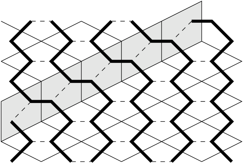
FIG. 4.: The mapping between the loop gas and the lozenge model: the shaded region shows an infinite line of defects.

FIG. 5.: Phase diagram of the loop gas in the $K-T$ plane; the solid lines denote the phase boundaries; the thick line represents the Lifshitz line; the dashed lines correspond to the disorder lines. The three phases are defined in the text.

FIG. 6.: Phase diagram of the loop gas in the $\rho-T$ plane; the solid lines denote the phase boundaries; the thick line represents the Lifshitz line; the dashed lines correspond to the disorder lines. The three phases are defined in the text.

REFERENCES

- [1] B. Nienhuis in Phase Transitions and Critical Phenomena, Vol. 11, ed. Domb and Lebowitz (Academic Press, New York 1987)
- [2] R. J. Baxter, Exactly Solved Models in Statistical Physics (Academic Press, New York 1982)
- [3] P.-G. G. de Gennes, Scaling Concepts in Polymer Physics (Cornell University Press, Ithaca 1979)
- [4] J. des Cloizeaux and G. Jannink, Polymers in Solution, their Modelling and Structure (Clarendon Press, Oxford 1990)
- [5] E. M. Lieb and F. Y. Wu in Phase Transitions and Critical Phenomena, Vol. 1, ed. Domb and Green (Academic Press, New York 1972)
- [6] J. P. Flory, Proc. Roy. Soc. A 234 60 (1956)
- [7] V. L. Pokrovsky and A. L. Talapov, Phys. Rev. Lett. 42, 65-67 (1979)
- [8] F. Y. Wu, Phys. Rev. 168 539-543 (1968)
- [9] H. W. J. Blöte and H.J. Hilhorst, J. Phys. A: Math. Gen. 15 L631-L637 (1982)
-
[10]
J. Stephenson, Can. J. Phys. 47 2621 (1969)
J. Stephenson, Can. J. Phys. 48 1724 (1970a)
J. Stephenson, Can. J. Phys. 48 2118 (1970b)
J. Stephenson, J. Math. Phys. 11 420 (1970c) - [11] R. M. F. Houtappel, Physica 16 425 (1950)
- [12] I. Syozi in Phase Transitions and Critical Phenomena, Vol. 1, ed. Domb and Green (Academic Press, New York 1972)
- [13] V. S. Dotsenko and V.S. Dotsenko, Advances in Physics 32, 129-172 (1983)
- [14] S. Samuel, J. Math. Phys. 21 2806-2814 (1980)
- [15] W. Helfrich, Z. Naturforsch. 33a, 305 (1978).
- [16] T. Garel and J.M. Maillard, J. Phys. C 19 L505-L511 (1986)
- [17] H. Saleur, J. Phys. A: Math. Gen. 19 2409-2423 (1986)