[

Superconducting Quantum Critical Point

Abstract

We study the properties of a quantum critical point which develops in a BCS superconductor when pair-breaking suppresses the transition temperature to zero. The pair fluctuations are characterized by a dynamical critical exponent $z=2$. Except for very low temperatures, anomalous contribution to the conductivity is proportional to $\sqrt{T}$ in three dimensions, but to $1/T$ in two dimensions. At lowest temperatures, the conductivity correction varies as $T^{1/4}$ in three dimensions, and as $\ln{(1/T)}$ in two.

] The possibility of quantum critical behavior in itinerant magnets has attracted great attention in recent years, in part, because quantum criticality affords the possibility of a controlled study of non-Fermi liquid behavior.[1] At a quantum critical point, order parameter fluctuations develop an infinite correlation range in both space and time.[2, 3] The coupling between these fluctuations and conducting electron fluid is able, under certain circumstances, to eliminate the formation of well-defined quasiparticles in the electron liquid, giving rise to a new kind of metallic behavior.

In this paper we discuss the possibility of quantum critical behavior in superconductors. A quantum critical point implies a finite value of the electron interaction strengths. At first sight, this would appear to rule out the possibility of a superconducting quantum critical point, for conventional superconductivity develops for an arbitrarily small pair interaction. If the transition temperature is driven to zero in a pure BCS superconductor, the pairing interaction and the pair fluctuations are completely eliminated. Fortunately, this is not the case in the presence of pair-breaking, which cuts off the logarithmic singularity in the pair susceptibility, requiring that the pairing interaction reach a critical strength before superconductivity develops. In this paper we characterize the quantum critical behavior which develops at this special point. Our results can be tested experimentally on conventional superconductors, such as $Ce$-doped $La$. [4] They may also provide a useful diagnostic tool for the understanding of unconventional, e.g. heavy fermion superconductors.

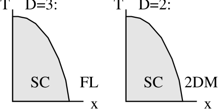
FIG. 1.: Schematic phase diagram in three ($D=3$) and in two ($D=2$) spatial dimensions. Shaded regions correspond to the superconducting (SC) phase. The normal phase corresponds to the Fermi liquid (FL) in three dimensions, and to a two-dimensional disordered metal (2DM) in two.

We begin with writing down the effective action of the pair field $\Delta$ in the vicinity of a quantum critical point:

$$S_{eff}[\Delta]=T\sum_{\nu,k}\Delta^{\dagger}\chi^{-1}\Delta+\frac{N(0)T^{3}}{T_{0}^{2}}\sum_{1,2,3}\Delta^{\dagger}_{1}\Delta^{\dagger}_{2}\Delta_{3}\Delta_{4},$$ (1)

$$\chi^{-1}=N(0)\left[\frac{\delta x}{x_{c}}+\left[\frac{T}{T_{0}}\right]^{2}+\frac{|\nu|}{T_{0}}+\left[\frac{v_{F}q}{T_{0}}\right]^{2}\right],$$ (2)

which is valid for $T,vq$, $|\nu|<<T_{0}$. Here $T$ is temperature, N(0) is the density of states at the Fermi surface, $\nu$ is a Matsubara frequency, $q$ is momentum, $v_{F}$ is the Fermi velocity, and $\delta x$ is the deviation of the control parameter $x$ from its critical value $x_{c}$, where the transition temperature turns into zero.

We obtained this action by repeating the Abrikosov-Gorkov calculation [5] for an $s$-wave BCS superconductor doped with magnetic impurities. Apart from the original calculation [5], the frequency and momentum dependence of the disorder-averaged pair propagator was kept and at the end both the pair field and the momentum were rescaled to give (1)-(2).

The quantity $T_{0}$ is the only characteristic energy scale of the effective action (1)-(2). In a BCS superconductor it is of the order of the pair-breaking rate, which at the critical point is of the order of the transition temperature in the clean system. Both quantities are much less than the Fermi energy $\epsilon_{F}$. However, in a strongly correlated material, $T_{0}$ may, in principle, be of the order of $\epsilon_{F}$.

These two limiting cases correspond to different physics. In the BCS case, the quartic term in (1) can be neglected at all experimentally relevant temperatures $T$ well below $T_{0}$. By contrast, if $T_{0}\sim\epsilon_{F}$, the feedback of the quartic term dominates at $T<<T_{0}$. In the latter case, one has to regard $T_{0}$ as a phenomenological parameter, resulting from a strong coupling, or non-BCS pairing mechanism.

TABLE I.: Order of magnitude and leading temperature dependences of the imaginary part of the electron self-energy $\Sigma(\omega;p=p_{F};T=0)$ due to scattering by the fluctuations of $\Delta$, the specific heat coefficient correction $\delta C(T)/T$ and the conductivity correction $\delta\sigma(T)$ in the weak coupling (BCS) limit ($T_{0}<<\epsilon_{F}$) and in the strong coupling limit ($T_{0}\sim\epsilon_{F}$). The value of $\sigma_{0}$ corresponds to the residual normal state conductivity.

	Electron	Specific Heat	Conductivity
	Self-Energy	Coefficient	Correction
	${\displaystyle Im\Sigma(\omega)}$	${\displaystyle\delta C(T)/T}$	${\displaystyle\delta\sigma(T)}$
$T_{0}<<\epsilon_{F},$
$d=3:$	${\displaystyle\frac{\left(T_{0}\omega\right)^{3/2}}{\epsilon_{F}^{2}}}$	${\displaystyle\frac{T_{0}^{3/2}T^{1/2}}{\epsilon_{F}^{3}}}$	${\displaystyle\sigma_{0}\frac{T_{0}^{3/2}T^{1/2}}{\epsilon_{F}^{2}}}$
$T_{0}\sim\epsilon_{F},$
$d=3:$	${\displaystyle\frac{\omega^{3/2}}{\epsilon_{F}^{1/2}}}$	${\displaystyle\frac{T^{1/2}}{\epsilon_{F}^{3/2}}}$	${\displaystyle\sigma_{0}\left(\frac{T}{\epsilon_{F}}\right)^{1/4}}$
$T_{0}<<\epsilon_{F},$
$d=2:$	${\displaystyle\frac{\omega T_{0}}{\epsilon_{F}}}$	${\displaystyle\frac{T_{0}}{\epsilon_{F}^{2}}\ln\left(\frac{T_{0}}{T}\right)}$	${\displaystyle\sigma_{0}\frac{T_{0}^{2}}{T\epsilon_{F}}}$
$T_{0}\sim\epsilon_{F},$
$d=2:$	${\displaystyle\omega}$	${\displaystyle\frac{1}{\epsilon_{F}}\ln\left(\frac{\epsilon_{F}}{T}\right)}$	${\displaystyle\sigma_{0}\ln\left(\frac{\epsilon_{F}}{T}\right)}$

With (1)-(2) at hand, one can calculate various thermodynamic and transport properties of interest. Table I presents the results for the zero-temperature quasiparticle decay rate due to scattering by the $\Delta$ field, and for the leading corrections to low-temperature thermodynamics and transport at $T_{c}=0$. In the BCS limit, corrections to the specific heat coefficient come from Gaussian fluctuations of the pair field.[6] The correction for a strong coupling case was found in [3] using renormalization group methods. The quasiparticle decay rate due to scattering off pair fluctuations is estimated by the diagram on Fig.2 (a). It is essential for the calculation of conductivity and of the quasiparticle decay rate, that the electron vertex corrections are not singular, since the pair-breaking makes the lifetime of a Cooper pair finite. The leading conductivity correction is given by the Aslamazov-Larkin diagram [7] shown on Fig.2(b), which can be regarded as conductivity of particles with the inverse propagator given by (2), at $\delta x=0$.

The calculation was done by renormalization group analysis of the expression for the Aslamazov-Larkin correction on Fig.2 (b). After transforming the Matsubara sum into a contour integral and going to dimensionless variables, it reads [8]:

$$\Delta\sigma=\int^{1}q^{2}d^{D}q\int^{1}\frac{dz}{T}\frac{1}{\sinh^{2}\frac{z}{2T}}\left[Im\chi(q,z+i0)\right]^{2},$$ (3)

where both the energy and the momentum cut-off have been set to unity. When renormalizing, we will follow [3]: first integrate out a thin outer shell in the momentum space between $1$ and $1-1/b$. Then rescale the momentum ($q\rightarrow qb$) to restore the cut-off, then rescale the energy ($z\rightarrow zb^{2}$), the mass term and the temperature ($T\rightarrow Tb^{2}$) and, finally, integrate out an energy shell to restore the energy cut-off. At each step the quartic interaction induces corrections to the mass term and to itself (see [3] for details of the renormalization group equations).

As a result, one arrives at the following transformation law for the Aslamazov-Larkin correction:

$$\Delta\sigma[J]=b^{2-D}\Delta\sigma[J^{\prime}]+\ln bf[J],$$

where $J$ denotes the mass term, the temperature and the quartic coefficient, $J^{\prime}$ denotes their renormalized values and $D$ is the dimensionality of the sample. The precise form of $f[J]$ can be easily obtained using the above renormalization procedure. However, only two features of $f[J]$ are important: (a) as long as the running value of $T$ is smaller than the cut-off, $f[J]$ has rather weak dependence on its arguments; this corresponds to the quantum renormalization region; (b) in the classical renormalization region, when $T$ exceeds the cut-off, $f[J]$ is proportional to $T$. Thus $\Delta\sigma$ can be written as

$$\Delta\sigma=\int_{0}^{\ln b^{*}}dxf[J(e^{x})]e^{(2-D)x},$$ (4)

where $b^{*}$ is the value of the rescaling factor at which the mass term reaches the cut-off and the scaling process stops. It is of the order of $T^{-3/4}$ in three dimensions and of the order of $\sqrt{\ln{(1/T)}/T}$ in two.[3] To evaluate (4), one also needs the value of $b_{1}$ such that $T(b_{1})\sim 1$, which is $b_{1}\sim T^{-1/2}$ independently of the dimensionality. With these prerequisites, the answers in Table I follow as soon as one neglects the dependence of $f[J(e^{x})]$ on all the couplings except temperature:

$$f[J(e^{x})]=f[Te^{2x}].$$

In three dimensions, the same result can be obtained just by replacing the “bare” $T^{2}$ mass term in (2) by its renormalized value $T^{3/2}$, and then calculating the conductivity correction as per (3).

Scaling analysis also allows to show that the vertex corrections are negligible. Their inclusion reduces to putting into the diagram of Fig.2 (b) extra bubbles such as one on Fig.2 (c). Each bubble contributes two Green’s functions plus an integral over the energy and momentum. After an infinitesimal scaling transformation, this gives an extra factor of $b^{2-D}$. Thus, in three dimensions, vertex corrections are irrelevant. In two dimensions, they appear marginal yet do not introduce any extra corrections. This can be established by using the Ward identity and writing the renormalization equation directly for the current vertex ( see Fig.3), and then inserting the solution into the corresponding expression for the conductivity.

We would like to discuss theoretical and experimental implications of the results. As envisaged by Hertz [2], under quite general circumstances the superconducting quantum critical point falls into the $z=2$ universality class. Although in principle different behavior cannot be ruled out, it appears to require additional tuning of parameters, as well as rather unusual features of the pairing phenomenon itself, such as the gap vanishing at the entire Fermi surface.[9]

In a weakly interacting disordered metal, $T_{0}$ in (2) is of the order of the impurity scattering rate. In this case anomalous corrections due to quantum criticality in the Landau-Ginzburg regime are of the order of the weak localization corrections.[10] Therefore, in two dimensions our results are fully consistent only as long as all corrections are small and additive. Moreover, in two dimensions, the electron-electron interaction is known to lead to the linear temperature dependence of the quasiparticle decay rate [10, 11], regardless of closeness to the quantum critical point. Thus, for a weakly interacting two-dimensional system, the entire normal region corresponds to the two-dimensional disordered metallic regime (see Fig.1) with the quasiparticle decay rate proportional to the quasiparticle energy.

However, we expect that in a strongly correlated system with suppressed weak localization effects, superconducting quantum critical point still falls into the $z=2$ universality class and Table I may describe the actual state of affairs for all dimensionalities. In this case, Fermi liquid turns marginal only at $T_{c}=0$ and crosses over to the normal Fermi liquid behavior as the system is driven away from the quantum critical point into the metallic phase.

Finally, we should like to comment on the diagnostic opportunities, furnished by measurements at a superconducting quantum critical point. In light of the discussion in the beginning of the paper, one is led to conclude that in a clean time reversal invariant system, observation of singular behavior at the superconducting quantum critical point would mark a very peculiar phenomenon, as in a clean BCS superconductor suppression of $T_{c}$ completely eliminates pair fluctuations. Since any sample contains impurities, in reality the above conclusion refers to temperatures above the elastic scattering rate: $T>\tau^{-1}$. The latter can be extracted from the residual resistivity measurements of the sample.

To summarize, we studied the properties of a superconductor near a quantum critical point driven by pair-breaking disorder. Superconducting fluctuations are characterized by a dynamical critical exponent $z=2$. In a BCS superconductor at experimentally accessible low temperatures, the singular contribution to the conductivity is proportional to $\sqrt{T}$ in three dimensions, but to $1/T$ in two dimensions. In a superconductor with the characteristic energy scale of the order of $\epsilon_{F}$ at the quantum critical point, the contribution to the conductivity varies as $T^{1/4}$ in three dimensions, and as $\ln{(1/T)}$ in two.

We are indebted to E. Abrahams, I. Aleiner, L. Glazman, G. Kotliar, A. Larkin, A. Millis, M. Stephen and A. Tsvelik for discussions related to this work, which was supported by the National Science Foundation under Grant number DMR-96-14999. We would like to thank the Theoretical Physics group at Oxford for the kind hospitality during the period when this work was completed.

FIG. 2.: (a) Graph for the quasiparticle self-energy due to scattering by pair fluctuations. Solid lines denote the pair propagator; thin line denotes the quasiparticle Green function. (b-c) Graphs for the conductivity correction: (b) the Aslamazov-Larkin graph (c) an example of a graph with vertex corrections. Scaling dimension of all such graphs is an integer multiple of $(2-D)$.

FIG. 3.: (a) Graph for the conductivity, including the current vertex, denoted by the dark triangle. (b) contribution to the free energy in the second order in the quartic term, which gives rise to renormalization of the current vertex.

REFERENCES

- [1] see J. Phys. Cond. Mat. 8, (1996), for exhaustive references.
- [2] John A. Hertz, Phys. Rev. B 14, 1165 (1976).
- [3] A. J. Millis, Phys. Rev. B 48, 7183 (1993).
- [4] M. B. Maple et al., Phys. Rev. Lett. 23, 1375 (1969).
- [5] A. A. Abrikosov, L. P. Gor’kov, Sov. Phys. JETP 12, 1243 (1961).
- [6] see, e.g., A. M. Tsvelik, Quantum Field Theory in Condensed Matter Physics, Cambridge University Press, 1995.
- [7] L. G. Aslamazov, A. I. Larkin, Sov. Phys. Solid State 10, 1104 (1968).
- [8] A. G. Aronov, S. Hikami, A. I. Larkin, Phys. Rev. B 51, 3880 (1995).
- [9] R. Ramazashvili, Phys. Rev. B 56, 5518 (1997), and references therein.
- [10] B. L. Altshuler, A. G. Aronov, in Electron-Electron Interactions in Disordered Systems, editors A. L. Efros and M. Pollak (Elsevier Science Publishers B. V., 1985).
- [11] E. Abrahams, P. W. Anderson, P. A. Lee, and T. V. Ramakrishnan, Phys. Rev. B 24, 6783 (1981);