CHIRALITY IN LIQUID CRYSTALS: FROM MICROSCOPIC ORIGINS TO MACROSCOPIC STRUCTURE
T.C. LUBENSKY, A.B. HARRIS, RANDALL D. KAMIEN,

AND GU YAN

Department of Physics and Astronomy, University of Pennsylvania, Philadelphia, PA, 19104

Molecular chirality leads to a wonderful variety of equilibrium structures, from the simple cholesteric phase to the twist-grain-boundary phases, and it is responsible for interesting and technologically important materials like ferroelectric liquid crystals. This paper will review some recent advances in our understanding of the connection between the chiral geometry of individual molecules and the important phenomenological parameters that determine macroscopic chiral structure. It will then consider chiral structure in columnar systems and propose a new equilibrium phase consisting of a regular lattice of twisted ropes.

Keywords: Chirality; Chiral Liquid Crystals; Columnar phases

1 Introduction

Chirality leads to a marvelous variety of liquid crystalline phases, including the cholesteric, blue, TGB, and Sm$C^{*}$ phases, with characteristic length scales in the “mesoscopic” range from a fraction of a micron to tens of microns or more. In spite of its importance, remarkably little is known about the connection between chirality at the molecular level and the macroscopic chiral structure of liquid crystalline phases. In particular, it is not possible at this time to predict the pitch $P$ (of order a micron) of a cholesteric phase from the structure of its constituent molecules. This talk will address some aspects of the molecular origins of chirality. It will also speculate about a possible new phase in chiral columnar or polymeric systems.

2 What is Chirality?

A molecule is chiral if it cannot be brought into coincidence with its mirror image[1]. Examples of chiral molecules and the achiral configurations from which they are derived are shown in Fig. 1. A chiral molecule must have a three dimensional structure. A linear, “one-dimensional,” or a flat, “planar,” molecule cannot be chiral. In particular a chiral molecule cannot be uniaxial. Nevertheless, the local structure of liquid crystals phases (including the cholesteric and other chiral phases) is nearly uniaxial. Indeed the phenomenology of most chiral phases can be explained in terms of the chiral Frank free-energy density,

$$f=\mbox{${{\footnotesize 1}\over{\footnotesize 2}}$}K_{1}(\nabla\cdot{\bf n})^{2}+\mbox{${{\footnotesize 1}\over{\footnotesize 2}}$}K_{2}[{\bf n}\cdot(\nabla\times{\bf n})]^{2}+\mbox{${{\footnotesize 1}\over{\footnotesize 2}}$}K_{3}[{\bf n}\times(\nabla\times{\bf n})]^{2}-h{\bf n}\cdot(\nabla\times{\bf n}),$$ (1)

expressed in terms of the Frank director ${\bf n}({\bf x})$ specifying the local direction of uniaxial molecular alignment at the space point ${\bf x}$. This free energy does not distinguish directly between truly uniaxial molecules and biaxial molecules that spin about some local axis so that their average configurations are uniaxial. Chirality in this free energy is reflected in the term $-h{\bf n}\cdot(\nabla\times{\bf n})$. The parameter $h$ is a chiral or pseudoscalar field that is nonzero only if the constituent molecules are chiral. It is a phenomenological parameter that may vary with temperature (or other external field such as pressure) and may even change sign. Note that the Frank free energy makes no explicit reference to the fact that a chiral molecule cannot be uniaxial. $h$ determines the length scale of equilibrium chiral structures. For example, the pitch wavenumber $k_{0}=2\pi/P$ of a cholesteric is simply $k_{0}=h/K_{2}$. Thus the chiral parameter $h$ can be identified with $K_{2}k_{0}$. It has units of energy/(length)², and one would naively expect it to have a magnitude of order $T_{NI}/a^{2}$, where $T_{NI}$ is the isotropic-to-nematic transition temperature and $a\approx 30$Å is a molecular length. The elastic constant $K_{2}$ does conform to naive expectations from dimensional analysis and is of order $T_{NI}/a$. Thus $h=(2\pi K_{2}/P)\approx 2\pi T_{NI}/(aP)$ is or order $[T_{NI}/a^{2}](a/P)$, which is $a/P\approx 10^{-3}$ times smaller than naive dimensional analysis would predict.

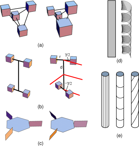
Figure 1: Examples of chiral structures created from achiral ones: (a) left, achiral tetrahedron with four equal masses at its vertices; right, a chiral tetrahedron with four unequal masses at its vertices. (b) left, an achiral planar “H”; right, a chiral “twisted H”. (c) left, an achiral propeller with all blades perpendicular to the hexagonal core; right, a chiral propeller with all blades rotated away from the normal to the hexagonal plane. (d) left, an achiral planar sheet; right, a helix formed by twisting a sheet about an cylinder. (e) left and middle, cylinder with achiral deorations; right, chiral cylinder with helical decorations.

The Frank free energy of Eq. (1) can be used to treat the cholesteric phase, chiral smectic phases (when a smectic free energy is added) and even low-chirality blue phases. To describe transitions from the isotropic phase to the cholesteric or blue phases, the Landau-de-Gennes free energy expressed in terms of the symmetric-traceless nematic order parameter $Q^{ij}$ is more useful. When there are chiral molecules, this free energy is

$$f_{Q} = \mbox{${{\footnotesize 1}\over{\footnotesize 2}}$}r{\rm Tr}Q^{2}-w{\rm Tr}Q^{3}+u{\rm Tr}Q^{4}$$ (2)

$$+\mbox{${{\footnotesize 1}\over{\footnotesize 2}}$}C_{1}\partial_{i}Q^{jk}\partial_{i}Q^{jk}+\mbox{${{\footnotesize 1}\over{\footnotesize 2}}$}C_{2}\partial_{i}Q^{ik}\partial_{j}Q^{jk}+H\epsilon^{ijk}Q^{il}\partial_{j}Q^{kl}.$$

The chiral term in this expression is the one proportional to the Levi-Civita symbol $\epsilon^{ijk}$. Indeed, the usual mathematical signal of chiral symmetry breaking in a free energy is a term linear in $\epsilon^{ijk}$. It is present in the Frank free energy in the term ${\bf n}\cdot(\nabla\times{\bf n})=\epsilon^{ijk}n^{i}\partial_{j}n^{k}$. In the nematic phase the order parameter $Q_{ij}$ is unixial: $Q^{ij}=S(n^{i}n^{j}-\mbox{${{\footnotesize 1}\over{\footnotesize 3}}$}\delta^{ij})$, where $S$ is the Maier-Saupe order parameter, and Eq. (2) reduces to Eq. (1) with $h\sim HS^{2}$. Thus, like the Frank free energy, the Landau-de-Gennes free energy makes no explicitly reference to biaxiality.

A theoretical goal should be the calculation of the parameter $h$ (or $H$) from molecular parameters and inter-molecular interactions. A theory should (1) show why $h$ is smaller than naive arguments would predict, (2) provide at least semi-quantitative guidance as to how molecular architecture affects $h$, and (3) elucidate the transition from necessarily non-uniaxial chiral molecules to an essentially uniaxial macroscopic free energy. Since $h$ is zero for achiral molecules, it is natural to expect that $h$ will be proportional to some parameter measuring the “degree of chirality” of constituent molecules. Section III will introduce various measures of molecular chirality and discuss why it is impossible to define a single measure of chirality. $h$ should depend on interactions between molecules as well as on chiral strength. Section IV will present a calculation of $h$ for simple model molecules composed of atoms interacting via classical central force potentials[2]. This calculation will highlight the role of biaxial correlations. It ignores, however, chiral quantum mechanical dispersion forces[3]. Finally, Sec. V will discuss chirality in columnar systems and speculate on the possibility of a new chiral phase consisting of a lattice of twisted ropes.

3 Measures of Molecular Chirality

To keep our discussion as simple as possible, we will consider only molecules composed of neutral atoms. All information about the symmetry of such a molecule can be constructed from its mass density relative to its center of mass:

$$\rho({\bf x})=\sum_{\alpha}m_{\alpha}\delta({\bf x}-{\bf r}_{\alpha}),$$ (3)

where $m_{\alpha}$ is the mass of atom $\alpha$ whose position vector relative to the molecular center of mass is ${\bf r}_{\alpha}$. A molecule is chiral if there exists no mirror operation $M$ under which $\rho({\bf x})$ is invariant, i.e., for all $M$, $\rho({\bf x})\neq\rho(M{\bf x})$. Mass moment tensors contain information about the symmetry and mass distribution of a molecule, and they can be used to construct chiral measures. The first moment specifies the position of the center of mass, which is uninteresting since we can always place the center of mass at the origin of our coordinates. Second- and third-rank moments are, however, interesting, and we define

$$C^{ij} = \sum_{\alpha}m_{\alpha}\left(r_{\alpha}^{i}r_{\alpha}^{j}-\mbox{${{\footnotesize 1}\over{\footnotesize 3}}$}r_{\alpha}^{2}\delta^{ij}\right),$$

$$C_{n}^{ij} = \sum_{\alpha}m_{\alpha}(r_{\alpha})^{n}\left(r_{\alpha}^{i}r_{\alpha}^{j}-\mbox{${{\footnotesize 1}\over{\footnotesize 3}}$}r_{\alpha}^{2}\delta^{ij}\right),$$ (4)

and

$$D^{klm} = \sum_{\alpha}m_{\alpha}\left[r_{\alpha}^{k}r_{\alpha}^{k}r_{\alpha}^{l}-\mbox{${{\footnotesize 1}\over{\footnotesize 5}}$}(r_{\alpha})^{2}(r_{\alpha}^{k}\delta^{lm}+r_{\alpha}^{l}\delta^{km}+r_{\alpha}^{m}\delta^{kl})\right],$$

$$D_{n}^{klm} = \sum{\alpha}m_{\alpha}(r_{\alpha})^{n}\left[r_{\alpha}^{k}r_{\alpha}^{k}r_{\alpha}^{l}-\mbox{${{\footnotesize 1}\over{\footnotesize 5}}$}(r_{\alpha})^{2}(r_{\alpha}^{k}\delta^{lm}+r_{\alpha}^{l}\delta^{km}+r_{\alpha}^{m}\delta^{kl})\right]{}.$$ (5)

where $(r_{\alpha})^{n}$ is $({\bf r}_{\alpha}\cdot{\bf r}_{\alpha})^{n/2}$. These tensors are symmetric and traceless, and they are invariant under the mirror operation that interchanges any two axes, say $x$ and $y$. Therefore, they cannot by themselves encode any information about molecular chirality.

To construct a quantity that is sensitive to chirality, we need combinations involving three distinct tensors in combination with the anti-symmetric Levi-Civita symbol $\epsilon^{ijk}$. One possible chiral parameter is
$\epsilon^{ijk}D^{ilm}C^{jl}(C^{2})^{km}$, where the Einstein convention on repeated indices is understood, and where $(C^{2})^{km}$ is the $km$ component of the tensor $C^{2}$. More useful chiral measures can be constructed by dividing $C^{ij}$ into a uniaxial and a biaxial part. The tensor $C^{ij}$ has five independent components that can be parametrized by two eigenvalues $\psi_{Q}$ and $\psi_{B}$ and an orthonormal triad $\{{\bf e}_{1},{\bf e}_{2},{\bf e}_{3}\}$ specifying the directions of the principal axes of the molecule. Thus, we can write

$$C^{ij}=Q^{ij}+B^{ij},$$ (6)

where

$$Q^{ij}=\psi_{Q}(e_{3}^{i}e_{3}^{j}-\mbox{${{\footnotesize 1}\over{\footnotesize 3}}$}\delta^{ij})\equiv\psi_{Q}{\tilde{Q}}^{ij}$$ (7)

and

$$B^{ij}=\psi_{B}(e_{1}^{i}e_{1}^{j}-e_{2}^{i}e_{2}^{j})\equiv\psi_{B}{\tilde{B}}^{ij}.$$ (8)

The last equation defines the reduced biaxial tensor ${\tilde{B}}^{ij}$ that depends only on the principal axis vectors ${\bf e}_{1}$ and ${\bf e}_{2}$. For a uniaxial molecule, the parameter $\psi_{B}$ is zero, and we will refer to $Q^{ij}$ as the uniaxial part of $C^{ij}$ and $B^{ij}$ as the biaxial part (even though the equilibrium average $\langle Q^{ij}\rangle$ can develop a biaxial part). The third rank tensor $D^{ijk}$ has seven independent components, which can be represented in the basis $\{{\bf e}_{1},{\bf e}_{2},{\bf e}_{3}\}$ defined by the principal axes of $C^{ij}$. Of these, only one component is of interest to the present discussion:

$$D^{klm}=\psi_{C}(e_{1}^{k}e_{2}^{l}e_{3}^{m}+5\,\,{\rm perm})\equiv\psi_{C}{\tilde{D}}^{klm}.$$ (9)

This equation defines the reduced third-rank tensor ${\tilde{D}}^{ijk}$. We can now introduce the chiral strength[2]

$$\psi=\epsilon^{ijk}e_{3}^{i}e_{3}^{l}B^{jm}D^{klm}=2\psi_{B}\psi_{D}=D^{xyz}(B^{xx}-B^{yy}).$$ (10)

This parameter clearly changes sign under any mirror operation. It must, therefore, be zero for any achiral molecule. It is a continuous function that has opposite signs for structures of opposite chirality. Consider, for example, the following mirror operations: (1) $z\rightarrow-z$, $D^{xyz}$ changes signs but $B^{xx}-B^{yy}$ does not; (2) $x\leftrightarrow y$, $(B^{xx}-B^{yy})$ changes sign but $D^{xyz}$ does not. More generally, we could introduce a class of chiral strength parameters defined in terms of $D_{n}^{klm}$ and the biaxial part, $B_{n}^{ij}$, of the tensor $C_{n}^{ij}$:

$$\psi_{pn}=\epsilon^{ijk}e_{3}^{i}e_{3}^{l}B_{p}^{jm}D_{n}^{klm}.$$ (11)

The parameter $\psi_{00}$ is equal to $\psi$. For all other $p$ and $n$, $\psi_{pn}$ is distinct from $\psi$.

It is instructive to calculate $\psi$ for some of the chiral molecules shown in Fig. 1. The “twisted H” structure is the simplest example of a geometrically chiral object. It has the pedagogical virtue that its geometric properties depend in a simple continuous way on the angle $\gamma$ between arms. When $\gamma=0$ or $\gamma=\pi/2$, the H is achiral. Thus any chiral measure must be zero at these points, and our expectation is that chiral measures will go continuously to zero at these points. Let $r$ be the radius of the arms of the “H” and $d$ be half its height. Then $\psi_{Q}=2(2d^{2}-r^{2})$, $\psi_{B}=2r^{2}\cos\gamma$, $\psi_{D}=2dr^{2}\sin\gamma$, and

$$\psi=4dr^{4}\sin 2\gamma.$$ (12)

As required, $\psi\rightarrow 0$ as $\gamma\rightarrow 0,\pi/2$. Another interesting example is the helix or spiral structure in Fig. 1(d). Parametrizing the helix by its position as a function of normalized arclength $s$: ${\bf R}(s)=[r\cos(2\pi ns),r\sin(2\pi ns),Ls]$, where $n$ is an integer, we find

$$\psi\approx{3r^{4}L\over(2\pi n)^{3}}\left[1-{24\over(\pi n)^{2}}\right].$$ (13)

Thus, $\psi$ decreases as the helix becomes more tightly wound ($n$ increases) - a reasonable result because at large distances a tightly wound spiral looks more like a uniform cylinder than does a not so tightly wound one.

There are many, in fact infinitely many, chiral strength parameters that provide a measure of the degree of chirality of a molecule. The set $\psi_{pn}$ defined above is just one of infinitely many sets we can define. At first, it may seem strange that the degree of chirality may be characterized in so many different ways. After all, chirality is simply the absence of a mirror symmetry, which involves a discrete operation. We might, therefore, have expected a single “chiral order parameter” analagous to the order parameter for an Ising model, which also describes the absence of a discrete symmetry. Chirality is, however, a function of the positions of all of the atoms in a molecule, which cannot be characterized by a single variable. Thus, chirality is perhaps more like the absence of spherical symmetry. There an infinite number of parameters, the spherical harmonics for example, that chracterize deviations from perfect sphericity.

Some measures of chirality are more useful than others, As we will see, the large-distance potential between two generic chiral molecules is directly proportional to the strength $\psi$ introduced in Eq. (10). Thus, $\psi$ provides a good measure of the strength of chiral interactions and enters into the calculations of $h$. There are molecules, such as the chiral tetrahedron of Fig. 1a, for which $\psi$ is zero. For such molecules, $\psi$ is clearly not very useful. Other measures are, however, nonzero and provide a measure of the strength of chiral interactions.

4 Chiral Pathways between Enantiomers

The mirror image of a chiral molecule is called its enantiomer. Any measure of chirality will change sign under a mirror operation, and as a result, chiral enantiomers will have chiral strengths of equal magnitude but opposite sign. This property implies that any series of continuous distortions of a molecule that takes it from a chiral configuration to that of its enantiomer must necessarily pass through a point where any given chiral measure is zero. It is tempting to conclude that this point corresponds to an achiral configuration and that any pathway between chiral enantiomers must pass through an achiral state. This conclusion is false. There are continuous pathways between chiral enantiomers all of whose states are chiral (for further discussion of this and the concept of a “topological rubber glove,” see [4]. A molecule is achiral if and only if any and all chiral measures are zero. For a particular chiral configuration, a given chiral measure may be zero, but at least one chiral measure be must be nonzero.

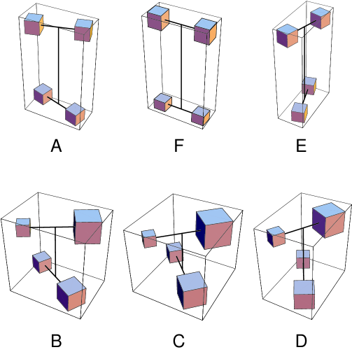
Figure 2: Pathways between chiral enantiomers consisting of $4$ atoms at the vertices of an H. $A$ and $E$ are chiral enantiomers (mirror images). The $4$ masses and their positions can be changed continuously to provide continuous pathways between the two enantiomers. Path $AFE$ passes through the achiral planar configuration $F$. Path $ABCDE$ passes through chiral configurations only. Configuration $C$ is the chiral tetrahedron with unequal masses.

To illustrate this point, let us consider the pathways depicted in Fig. 2 between reflected images of a twisted H. $A$ is a twisted H with an angle $\gamma=\pi/6$ between top and bottom arms. $E$ is its chiral enantiomer with angle $-\pi/6$ between arms. $F$ is the the achiral planar structure. $B$ through $D$ are all chiral configurations with different masses at the vertices of the H. $C$ is the chiral tetrahedron with four unequal masses. The path $AFE$ between chiral enantiomers passes through the achiral configuration $F$ for which all chiral measures are zero. On the other hand, all configurations in the path ABCDE are chiral even though $A$ and $E$ are chiral enantiomers for which any chiral measure $\psi$ must have opposite signs: $\psi(E)=-\psi(A)$. Thus, any continuous chiral measure must pass through zero at some point on the path $ABCDE$, but different chiral measures do not have to pass through zero at the same point. To illustrate these facts, we consider a specific parametrization of the closed path $ABCDEFA$. Let the four masses in the twisted H be

$$\{m_{1},m_{2},m_{3},m_{4}\}=m[\{1,1,1,1\}+\mu\{0.31,-0.31,0.23,-0.23\}].$$ (14)

The configurations of the twisted H are thus specified by the three parameters $\mu$, $d/r$, the ratio of the semiheight to the arm radius, and $\gamma$, the angle between the arms of the H. The following properties of a chiral measure $\psi$ are apparent:

1. $\mu=0$: Equal masses

   1. $\gamma=0$, $\gamma=\pi/2$: achiral $\Rightarrow$ $\psi=0$

   2. $d=r\sin(\gamma/2)$ or $d=r\cos(\gamma/2)$: achiral $\Rightarrow\psi=0$

   3. $\psi(\gamma)=-\psi(-\gamma)=-\psi(\pi-\gamma)=2dr^{4}\sin 2\gamma$.

2. $\mu\neq 0$: Unequal masses

   1. $\gamma=0$: planar achiral molecule $\Rightarrow\psi=0$

   2. $\gamma\neq 0$: chiral molecule $\Rightarrow\psi\neq 0$

   3. $\psi(\gamma,\mu)=\psi(\gamma,-\mu)$

   4. $d=r/\sqrt{2}$: chiral tetrahedron with unequal masses.

The points in Fig. 2 correspond to the following values of $[\gamma,\mu,d/r]$: $A=[\pi/6,0,1]$, $B=[\pi/3,3/4,(\sqrt{2}+3)/(4\sqrt{2})]$, $C=[0,1,1/\sqrt{2}]$, $D=[2\pi/3,3/4,(\sqrt{2}+3)/(4\sqrt{2})]$, $E=[5\pi/6,0,1]=[-\pi/6,0,1]$. Figure 3a shows the normalized chiral strengths $\Psi_{nm}=\psi_{nm}(\gamma,\mu,d/r)/\psi(A)$ for $(n,m)=(0,0)$ and $(n,m)=(0,8)$ as a function of $\gamma$ for the path $EFA$ with $\mu=0,d/r=1$. Only one curve appears in the figure because the two curves for $\Psi_{00}$ and $\Psi_{08}$ are identical. As required, the curve passes through zero at the achiral point $\gamma=0$. Figures 3a and 3b show the normalized strengths $\Psi=\Psi_{00}$ and $\Psi_{08}$ for the path $ABCDE$ with $\pi/6\leq\gamma\leq 5\pi/6$ with $\mu=1-(9/4)[(2\gamma/\pi)-1]^{2}$ and $d/r=(1\sqrt{2})+(9/4)[1-(1/\sqrt{2})][(2\gamma/\pi)-1]^{2}$. The two curves are clearly different, but they appear to go to zero at $\gamma=\pi/2$. Figure 3d shows a blowup of the region around $\gamma=\pi/2$, showing that $\Psi$ and $\Psi_{08}$ pass through zero at different values of $\gamma$. Note that $\Psi$ passes through zero at $\gamma=\pi/2$ indicating that this parameter does not provide a measure of the chirality of the tetrahedron with unequal masses. $\Psi_{08}$ is nonzero but small at $\gamma=\pi/2$.

Figure 3: Plots of reduced chiral strength parameters for different pathways between chiral enantiomers shown in Fig. 2. (a) $\Psi=\psi_{00}/\psi_{00}(A)=\psi_{08}/\psi_{08}(A)$ for the path $EFA$ passing through the achiral configuration $F$. (b) $\Psi=\psi_{00}/\psi_{00}(A)$ for the path $ABCDE$. (c) $\Psi_{08}=\psi_{08}/\psi_{08}(A)$ for the path $ABCDE$. (d) $\Psi$ and $\Psi_{08}$ in the vicinity of $\gamma=\pi/2$. They pass through zero at different points.

The path $ABCDE$ was chosen to pass through the chiral tetrahedron at point $C$. A tetrahedrally coordinated carbon atom bonded to four differenct atoms or chemical groups is a chiral center. It is used to identify chriality in molecules. Interestingly, the simple chiral tetrahedron is not very chiral according to the measures $\psi_{pn}$. All measures $\psi_{00}$ to $\psi_{05}$ are zero for this molecule. This is a partial explanation of why the difference between $\Psi$ and $\Psi_{08}$ is so small near $\gamma=\pi/2$. Other pathways between $A$ and $E$ would display more pronounced differences.

5 Calculation of $h$

Two distinct microscopic mechanisms contribute to a non-vanishing macroscopic chiral parameter $h$. The first is quantum mechanical in origin and has its clearest manifestation in the generalization of the familiar Van der Waals dispersion potential to chiral molecules[3]. The electrostatic potential between molecules is expanded to include dipole-quadrupole as well as dipole-diple interactions. The expectation value of the dipole-moment–quadrupole-moment product $\langle p^{i}Q^{jk}\rangle$ is nonzero for a chiral molecules and is proportional to $(\epsilon^{ijl}e_{3}^{l}e_{3}^{k}+{\rm perm})$ for a molecule spun about the direction ${\bf e}_{3}$. The resultant potential has the form,

$$U=V(R){\bf e}_{3}\cdot{\bf e}_{3}^{\prime}{\bf e}_{3}\cdot({\bf R}\times{\bf e}_{3}^{\prime}),$$ (15)

where $R$ is the spatial separation of the centers of mass of the two molecules and $V(R)\sim R^{-7}$. This potential leads directly to the Landau-de-Gennes chiral interaction $\epsilon^{ijk}Q^{il}\partial^{j}Q^{kl}$ in the isotropic phase [Eq. (2)] and to the Frank chiral term in the nematic phase with $h\sim S^{2}$. The calculation of the strength of the potential $V(R)$ for real liquid crystal molecules is complex. The second mechanism can be described in purely classical terms. It arises from central force potentials, including hard-core potentials, between points (or atoms) on molecules with chiral shapes. This is the mechanism popularized by Straley’s[5] image of two interlocking screws that twist relative to each other. Here we will consider only the second mechanism. We will show that $h$ is nonzero only if there are biaxial correlations between molecules and as a consequence is zero in any mean-field theory with uniaxial order parameters.

We consider each molecule $A$ to be composed of atoms $\alpha$ whose positions within the molecule are rigidly fixed. Atoms on different molecules interact via a central potential $V(R)$. Let ${\bf R}_{A}$ be the position of the center of mass of molecule $A$, ${\bf r}_{A\alpha}$ be the position of atom $\alpha$ relative to ${\bf R}_{A}$, and ${\bf R}_{A\alpha}={\bf R}_{A}+{\bf r}_{A\alpha}$ be the position of atom $\alpha$ in molecule $A$. The total intermolecular potential energy is thus

$$U=\mbox{${{\footnotesize 1}\over{\footnotesize 2}}$}\sum_{A\alpha\neq B\beta}V(|{\bf R}_{A\alpha}-{\bf R}_{B\beta}|).$$ (16)

The chiral parameter $h$ is the derivative of the free energy density with respect to the cholesteric wave number $k=2\pi/P$ evaluated in the aligned state with spatially uniform director ${\bf n}$ and $k=0$:

$$h=-\left.{\partial f\over\partial k}\right|_{k=0}=-{1\over\Omega}\left.\left\langle{\partial U\over\partial k}\right\rangle\right|_{k=0}=-{1\over 4\Omega}\sum_{BA}T_{BA},$$ (17)

where $\Omega$ is the system volume and

$$T_{BA}=\left\langle\sum_{\beta\alpha}\epsilon^{ijk}R_{\perp}^{i}r_{\beta}^{j}\partial^{k}V({\bf R}+{\bf r}_{\beta}-{\bf r}_{\alpha})\right\rangle$$ (18)

is the “projected torque”, ${\bf R}_{\perp}\cdot{\mbox{\boldmath{$\tau$}}}_{AB}$, where ${\mbox{\boldmath{$\tau$}}}_{AB}$ is the torque exerted on $A$ by $B$. Here ${\bf r}={\bf R}_{B}-{\bf R}_{A}$ and ${\bf r}_{\perp}$ is the component of ${\bf r}$ perpendicular to the uniform director ${\bf n}$. This expression for $h$ is quite general. It can be used in Monte Carlo and molecular dynamics simulations. It is valid both classically and quantum mechanically. (It will reproduce the dispersion calculations described above if electron as well as atomic coordinates are included). Here we restrict our attention to classical central forces. The fundamental question is, how do nonchiral central forces give rise to effective chiral forces? To answer this question, we consider the multipole expansion of $U$. Schematically, we have

$$\sum_{\alpha,\beta}V({\bf R}_{A\alpha}-{\bf R}_{B\beta}) \rightarrow \mbox{${{\footnotesize 1}\over{\footnotesize 4}}$}[\partial^{i}\partial^{j}\partial^{k}\partial^{l}V]C_{A}^{ij}C_{B}^{kl}$$

$$+\mbox{${{\footnotesize 1}\over{\footnotesize 24}}$}[\partial^{i}\partial^{j}\partial^{k}\partial^{l}\partial^{m}V](C_{A}^{ij}D_{B}^{klm}+C_{B}^{ij}D_{A}^{klm}).$$

The second term on the right hand side of this equation is the chiral term. It can be expressed as

$$V_{C}=\mbox{${{\footnotesize 1}\over{\footnotesize 24}}$}\psi_{D}\psi_{B}[\partial^{i}\partial^{j}\partial^{k}\partial^{l}\partial^{m}V]({\tilde{B}}_{A}^{ij}{\tilde{D}}_{B}^{klm}+{\tilde{B}}_{B}^{ij}{\tilde{D}}_{A}^{klm}),$$ (20)

where the reduced tensors ${\tilde{B}}^{ij}$ and ${\tilde{D}}^{klm}$ are defined in Eqs. (8) and (9). The triad of vectors $\{{\bf e}_{1},{\bf e}_{2},{\bf e}_{3}\}$ forms a right-handed coordinate system. Since this triad is determined by the second-moment tensor, it can be chosen to be invariant under a chiral operation $M$. Thus, the reduced tensors ${\tilde{B}}^{ij}$ and ${\tilde{D}}^{klm}$ do not change sign under a chiral operation. The chiral parameter $\psi=2\psi_{B}\psi_{D}$ and the potential $\partial^{5}V$ both change sign under a chiral operation on all atoms. Thus the potential $V_{C}$ is invariant under a chiral operation involving all atoms. If, however, we perform a chiral operation about the center of mass of each molecule (i.e., convert each molecule to its enantiomer) leaving the centers-of-mass positions fixed, $\psi$ changes sign but $\partial^{5}V$ remains unchanged. Thus, the potential $V_{C}$ changes sign upon reversing the chirality of constituent molecules. As we noted earlier, any term linear in the Levi-Civita symbol $\epsilon^{ijk}$ is chiral. The potential $V_{C}$ is linear in $\epsilon^{ijk}$ because the triad $\{{\bf e}_{1},{\bf e}_{2},{\bf e}_{3}\}$ is right handed, and ${\bf e}_{1}=({\bf e}_{2}\times{\bf e}_{3})$, ${\bf e}_{2}=({\bf e}_{3}\times{\bf e}_{1})$, and ${\bf e}_{3}=({\bf e}_{1}\times{\bf e}_{2})$. Thus

$${\tilde{D}}^{ijk}=\epsilon^{ilm}e_{3}^{j}e_{3}^{l}{\tilde{B}}^{km}+\epsilon^{klm}e_{3}^{i}e_{3}^{l}{\tilde{B}}^{jm}+\epsilon^{jlm}e_{3}^{k}e_{3}^{l}{\tilde{B}}^{im}.$$ (21)

We now consider the evaluation of $h$ from Eq. (17) and the multipole expansion of Eq. (5). To simplify our calculation, we restrict all molecular axes ${\bf e}_{3A}$ to be rigidly aligned along a common axis ${\bf n}_{0}$. This is equivalent to forcing the Maier-Saupe order parameter $S$ to be unity. In this case, the potential $V_{C}$ involves only the product of the biaxial moment ${\tilde{B}}^{ij}$ on different molecules, and upon averaging, the torque becomes

$$T_{BA}=\psi\langle K(R)\Gamma_{B}(R)\rangle,$$ (22)

where

$$\Gamma_{B}(R)=\langle{\tilde{B}}_{B}^{ij}{\tilde{B}}_{A}^{ij}\rangle=2\langle\cos 2(\phi_{B}-\phi_{A})\rangle$$ (23)

is the biaxial correlation function and

$$K(R)=R_{\perp}^{2}\left\{g^{(3)}+R_{||}^{2}g^{(4)}+\mbox{${{\footnotesize 1}\over{\footnotesize 4}}$}R_{\perp}^{2}[g^{(4)}+R_{||}^{2}g^{(5)}]\right\},$$ (24)

where $g(R^{2}/2)=V(R)$, and $g^{(n)}(x)=d^{n}g(x)/dx^{n}$. If molecules rotate independently, the biaxial correlation function $\Gamma_{B}({\bf R})$ is zero. Mean-field theory seeks the best single particle density matrix and thereby ignores correlations between different particle. Thus, in mean-field theory, $\Gamma_{B}$ is zero, and the chiral potential $h$ is zero unless there is long-range biaxial order with a nonvanishing value of $\langle\cos 2\phi_{A}\rangle$. The latter observation was made some time ago[6, 7]. Nevertheless, there have since been mean-field calculations claiming to produce a nonvanishing $h$ in a uniaxial system[8]. In uniaxial systems, $\Gamma_{B}(R)\propto e^{-R/\xi}$ where $\xi$ is the biaxial correlation, which should be order a molecular spacing. We can now provide a partial answer to the question of why $h$ is so much smaller than naive scaling arguments would predict. First, the chiral strength $\psi$ may be quite small, particularly for tightly would helical molecules such as DNA or tobacco mosaic viruses. Second, the biaxial correlation length could be small (because, for example the molecules are only weakly biaxial), allowing only very near neighbors to contribute to the sum over $AB$ in Eq. (17) for $h$.

6 Chiral Columnar Phases

We now have a fairly complete catalog and understanding of equilibrium phases of rod-like chiral mesogens. Our understanding of chiral phases of disc-like chiral mesogens is less complete. Such mesogens have been synthesized[9, 10]. They produce cholesteric and columnar mesophases, the latter of which exhibit unusual spiral textures[9]. Columnar phases with spontaneous chiral symmetry breaking in which propeller-like molecules rotate along columns have been observed[11]. In addition, long, semi-flexible polymers like DNA whose natural low-temperature phase has columnar symmetry, exhibit cholesteric, columnar, and blue phases[12], and even what appears to be a hexatic phase[13]. There have been theoretical predictions of a number of phases including (1) a moiré phase[14] in which the hexagonal columnar lattice rotates in discrete jumps about an axis parallel to the columns across twist grain boundaries consisting of a honeycomb lattice of screw dislocations, (2) a tilt-grain boundary phase[14] in which columns rotate in discrete jumps bout an axis perpendicular to the columns across twist-grain boundaries consisting of a parallel array of screw dislocations, and (3) a soliton phase[15] in which molecules all rotate in the same sense in their columns without disrupting the regular hexagonal columnar lattice. Many other states are possible. Here we will consider one of them: a hexagonal lattice of twisted ropes. This phase would be constructed as follows: First, take cylindrical sections of radius $R$ of a columnar lattice and twist them about an axis parallel to the columns as shown in Fig. 4. This operation will cost strain energy but will gain twist energy. Next put these columns on a regular hexagonal lattice and deform the cylinders to a hexagonal shape to produce a dense packing as shown in Fig. 5. The interface between adjacent hexagonal cylinders is a twist grain boundary and is favored if chiral interactions are sufficiently strong. On the other hand, there is a strain energy cost associated with distorting the cylinders and an energy cost associated with the vertices of the hexagons. The radius of the original cylinders (and thus the lattice spacing) and the degree of twist within a cylinder will adjust to minimize the free energy. This lattice of twisted ropes should be competitive with the moiré, tilt-grain-boundary, and soliton phases.

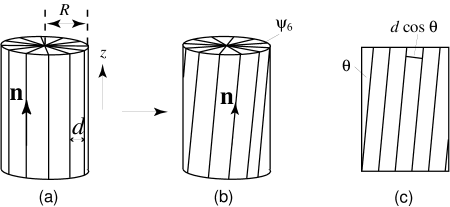
Figure 4: Twisting a cylinder of a columnar lattice. (a) The untwisted cylinder of radius $R$ with equilibrium spacing between columns $d$. (b) The twisted cylinder. (c) The outer surface of the twisted cylinder unrolled. The columns make an angle $\theta=\tan^{-1}k_{0}R$ with respect to the cylindrical axis. The normal spacing between between layers is now $d/\cos\theta\approx d(1+\theta^{2}/2)$.

To be more quantitative, we now investigate in more detail the various contributions to the energy of this lattice. The elastic energy density of a columnar phase with columns aligned along the $z$ axis is

$$f_{\rm el}=\mbox{${{\footnotesize 1}\over{\footnotesize 2}}$}\lambda u_{\alpha\beta}^{2}+\mu u_{\alpha\beta}u_{\alpha\beta}+\mbox{${{\footnotesize 1}\over{\footnotesize 2}}$}K_{3}(\partial_{x}{\bf u})^{2}+\mbox{${{\footnotesize 1}\over{\footnotesize 2}}$}K_{6}(\nabla\theta_{6})^{2},$$ (25)

where

$$u_{\alpha\beta}=\mbox{${{\footnotesize 1}\over{\footnotesize 2}}$}(\partial_{\alpha}u_{\beta}\partial_{\beta}u_{\alpha}+\partial_{\gamma}u_{\alpha}\partial_{\gamma}u_{\beta}-\partial_{z}u_{\alpha}\partial_{z}u_{\beta}),\,\,\alpha,\beta=x,y$$ (26)

is the nonlinear strain for a columnar lattice in mixed Euler-Lagrangian coordinates. The first three terms in this nonlinear strain are identical to the nonlinear Lagrangian strain (with a relative plus sign between the linear and nonlinear terms) of a two-dimensional solid in which the coordinates $x$ and $y$ refer to positions in a reference unstrained sample. The third term reflects the three-dimensional nature of the columnar phase. There is a minus sign between it and the preceding terms because $z$ measures a coordinate in space and not a coordinate in a reference solids; it is an Eulerian rather than a Lagrangian variable[16]. The variable $\theta_{6}=(\partial_{x}u_{y}-\partial_{y}u_{x})/2$ in Eq. (25) specifies the direction of hexatic order of the lattice. In a chiral system, there are additional chiral terms in the free energy density:

$$f_{\rm ch}=-\gamma_{\theta}\partial_{z}\theta_{6}-\gamma_{n}{\bf n}\cdot(\nabla\times{\bf n}),$$ (27)

where ${\bf n}$ is the nematic director, which is parallel to the local columnar axis. The first term in $f_{\rm ch}$ favors twisting of the hexagonal columnar lattice along the columns, i.e., it favors a twisted rope or the moiré configuration. The second term favors twisting of the columns along directions perpendicular to the local columnar axes, i.e., it favors a tilt-grain-boundary structure.

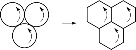
Figure 5: Close-packed twisted cylinders deformed to spacefilling hexagonal twisted cylinders.

We can use $f_{\rm el}$ and $f_{\rm ch}$ to calculate the preferred configuration of a cylinder of a chiral columnar lattice of radius $R$ in which dislocations and other defects are not allowed. The elastic energy of a lattice in which $\theta_{6}=k_{0}z$ is uniformly twisted with twist wavenumber $k_{0}$ is controlled by the nonlinear term $\partial_{z}u_{\alpha}\partial_{z}u_{\beta}$ of the strain. Indeed the two-dimensional Lagrangian part of the strain arising from such a uniform twist is zero! There are nonlinear contributions to the strain, however, because the distance between neighboring columns increases as the columns are twisted as depicted in Fig. 4. Since twisting produces no linear strain, the energy required to twist a columnar lattice is lower than that required to twist a three-dimensional elastic solid. The elastic energy per unit length of a twisted columnar lattice can be calculated. For small $k_{0}R$, it is

$${E_{\rm el}\over L}={\overline{\mu}}(k_{0}R)^{4}\pi R^{2}+\mbox{${{\footnotesize 1}\over{\footnotesize 4}}$}K_{3}k_{0}^{2}(k_{0}R)^{2}\pi R^{2}+\mbox{${{\footnotesize 1}\over{\footnotesize 2}}$}K_{6}k_{0}^{2}\pi R^{2}.$$ (28)

where $\overline{\mu}$ is an effective modulus that is strictly proportional to $\mu$ in an incompressible system where the bulk coefficeint $\lambda$ is infinite. This energy should be compared to the result, $\mu k_{0}^{4}R^{4}$, for a three-dimensional solid. The chiral energy per unit length is

$${E_{\rm ch}\over L}=-[\gamma_{\theta}k_{0}+\gamma_{n}k_{0}(k_{0}R)^{2}]\pi R^{2}.$$ (29)

Equations (28) and (29) can be used to determine the twist wavenumber $k_{0}$ for a cylindrical rod of radius $R$.

Our goal is to determine the lowest energy lattice of rods for given values of the coupling constants. We begin by distorting our cylindrical rods into hexagonal rods so that they can pack closely in an hexagonal array (Fig. 5). Each unit cell of the lattice is now a hexagonal cylinder of twisted columns. This distortion will cost an energy for each rod proportional to its shear modulus times its volume $\pi R^{2}L$: $E_{\rm dist.}=\alpha\mu\pi R^{2}L$, where $\alpha$ is a constant of order unity. The columns at the outer edge of the hexagonal unit cells make an angle of $\theta=\tan^{-1}k_{0}R\approx k_{0}R$ relative to the vertical $z$ axis. Columns on opposite sides of a boundary between adjacent hexagonal unit cells, however, make opposite angles relative to this axis, so the boundary is in fact a twist grain boundary across which the columnar lattice undergoes a change in angle of $2\theta$ as shown in Fig. 6.

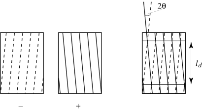
Figure 6: Creation of a twist grain boundary at the interface between two cells. All cells twist in the same direction. The columns in back (-) and in from (+) of a given interface twist in opposite directions. The interface is thus a twist grain boundary consisting of screw dislocations perpendicular to the $z$ axis separated by a distance $l_{d}=d/2\sin\theta$, where $2\theta$ is the change in angle of the columnar lattice across the boundary.

There is a positive energy cost to a grain boundary coming from the cost of creating the dislocations in the boundary. There is also an energy gain in chiral systems arising from the $-\gamma_{n}{\bf n}\cdot(\nabla\times{\bf n})$ term in $f_{\rm ch}$. Consider a boundary in the $xz$ plane with dimensions $L_{x}\times L_{z}$. Since $\int dy{\bf n}\cdot\nabla\times{\bf n}=L_{x}L_{z}2\theta$, where the integral is across the grain boundary, there is a chiral energy gain of $-\gamma_{n}L_{x}L_{z}2\theta\approx-\gamma_{n}L_{x}L_{z}2k_{0}R$. The dislocation energy is $E_{\rm disc}=N_{d}L_{x}\epsilon$, where $\epsilon$ is the energy per unit length of a dislocation, and $N_{d}=L_{z}/l_{d}$ is the number of dislocations with $l_{d}$ the distance between dislocations. There is a simple geometric relation between $l_{d}$ and $\theta$: $\theta=\sin^{-1}d/2l_{d}\approx d/2l_{d}$, where $d$ is the spacing between columns in the columnar lattice. Thus the energy of a grain boundary for small $k_{0}R$ is $E_{\rm GB}=L_{x}L_{z}(\epsilon d^{-1}-2\gamma_{n})2k_{0}R$. The length $L_{x}$ is proportional to $R$: $L_{x}=a\pi R/3$, where $a$ is a constant of order unity. The first term in $f_{\rm ch}$ contributes an energy $-\pi R^{2}L_{z}\gamma_{\theta}k_{0}$ per column. Finally, there is an energy per unit length $\tau/2$ for each vertex of the hexagonal lattice where grain boundaries meet. Combining all of these energies and keeping only the dominant terms, we find

$$f={E\over V}={\overline{\mu}}(k_{0}R)^{4}-\gamma k_{0}+{\tau\over R^{2}}+\alpha\mu,$$ (30)

where $\gamma=\gamma_{\theta}+(4a/3)(\gamma_{n}-\epsilon d^{-1})$. Minimization of this energy over $k_{0}$ for $\gamma>0$ yields

$$k_{0}=\left({\gamma\over 4{\overline{\mu}}R^{4}}\right)^{1/3}\sim R^{-4/3}.$$ (31)

Thus $k_{0}R\sim R^{-1/3}$ is much less than one when $\gamma$ is small and $R$ is large. At this optimal value for $k_{0}$,

$$f=-{3\over 4}\gamma\left({\gamma\over 4{\overline{\mu}}}\right)^{1/3}R^{-4/3}+{\tau\over R^{2}}+\alpha\mu.$$ (32)

Minimization over $R$ yields

$$R={(8{\overline{\mu}}\tau)^{3/2}\over\gamma^{2}}$$ (33)

and

$$f=-{1\over 64}{\gamma^{4}\over{\overline{\mu}}\tau^{2}}+\alpha\mu.$$ (34)

Thus, for sufficiently strong chiral coupling $\gamma$, this free energy will be lower than that of a uniform columnar phase with no twist, and it is possible that there is some range of parameters for which this phase has a lower energy than either the moiré or the soliton phase.

ABH was supported by NSF Grant Number 95-20175. RDK and TCL were supported by NSF Grant Number DMR94-23114 and by the Materials Science and Engineering Center Program of NSF under award number DMR96-32598.

References

- [1] W. Thomson, The Robert Boyle Lecture, Oxford University Junior Scientific Club, May 16, 1893, reprinted in Baltimore Lectures, (C.J. Clay & Sons, London, 1904).
- [2] A.B. Harris, Randall D. Kamien, and T.C. Lubensky Phys. Rev. Lett. 78 1476-1479 (1997), cond-mat/9611224.
- [3] B.W. Van der Meer, G. Vertogen, A.J. Dekker, and J.G.J. Ypma, J. Chem. Phys. 65, 3935 (1976); E.I. Kats, Zh. Eksp. Teor. Fiz. 74, 2320-30 (1978)
- [4] D.M. Walba, in Chemical Applications of Topology and Graph Theory, edited by R.B. King (Elsevier, Amsterdam, 1983); David M. Walba, Timothy C. Homan, Rodney M. Richards, and R. Curtis Haltiwanger in Chemistry: Knots and Applications, edited by Louis H. Kaufman (World Scientific, Singapore, 1995). [Sov. Phys. JETP 47, 1205-10 (1978)].
- [5] J.P. Straley, Phys. Rev. A 14, 1835 (1976).
- [6] H. Schröder, The Molecular Physics of Liquid Crystals, ed. by G.R. Luckhurst and G.W. Gray (Academic Press, New York, 1979) Chap. 5.
- [7] W.J.A Goossens, Mol. Crys. Liq. Cryst. 12, 237 (1971)
- [8] Glenn T. Evans, Mol. Phys. 77, 969-81 (1992)
- [9] J. Malthête, J. Jacques, Nguyen Tinh, and C. Destrade, Nature 298, 46 (1982); G. Scherowskyu and Xin Hua Chen, Liquid Crystals 17, 803 (1994); K. Praefcke, D. Singer, and A. Eckert, Liquid Crystals 16, 53–65 (1994).
- [10] H. Bock and W. Helfrich, Liquid Crystals 18, 387 (1995); “Field dependent switching angle of a columnar pyrene,” ibid. 707.
- [11] E. Fontes, P.A. Heiney, and W.H. de J, Phys. Rev. Lett. 61, 1202 (1988); P.A. Heiney, E. Fontes, W.H. de Jeu, P. Carroll, and A.B. Smith III, J. Phys. France 50, 461 (1989)
- [12] F. Livolant, Physica A 176, 117–37 (1991).
- [13] R. Podgornik, H.H. Strey, K. Gawrisch, D.C. Rau, A Rupprecht, and V.A. Parsegian, Proc. Nat. Acad. Sci. 93, 4261 (1996).
- [14] Randall D. Kamien and D.R. Nelson, Phys. Rev. Lett. 74, 2499 (1995), cond-mat/9411039; Phys. Rev. E 53, 650 (1996), cond-mat/9507080.
- [15] Gu Yan and T.C. Lubensky, J. Phys. II France 7, 1023–34, (1997), cond-mat/9611066.
- [16] P.M. Chaikin and T.C. Lubensky, Principles of Condensed Matter Physics” (Cambridge Press, Cambridge, 1994), Chap. VI.