A lattice gas model of avalanches in a granular pile

Abstract

A granular media lattice gas (GMLG) model is used to study avalanches in a two-dimensional granular pile. We demonstrate the efficiency of the algorithm by showing that several features of the non-critical behaviour of real sandpile surfaces, such as the bounded outflow statistics or the finite-size effect of the time evolution of the pile mass, can be reproduced by this simulation approach.

The concept of self-organized criticality (SOC) [1] has become popular in the research of non-equilibrium systems. According to this idea, weakly driven non-equilibrium systems can spontaneously organize themselves into a state of diverging characteristic length and time scales. It was suggested that avalanches on sandpile surfaces may fit into the SOC framework and this idea inspired considerable activity in the field of the physics of granular materials.

Sandpiles soon proved to behave differently from the proposed picture in many aspects. Avalanches in a rotating drum were found to occur at well-defined interwalls and the probability density of avalanche durations turned out to be sharply peaked [2]. Using a different experimental setup, where grains were dropped onto the top of a conical pile, Held et al.  did find scaling in small piles[3]. However, if the size of the pile was above a certain value, the small fluctuations disappeared from the system. The crossover to this quasi-regular behaviour can be explained by the fact, that the surface of the pile has two characteristic angles rather than a single one: the angle of repose and the angle of marginal stability. In the case of sufficiently small piles the size of one single particle is large enough to raise the local angle above the critical value and therefore no hysteresis can be found[4]. Further measurements pointed out that the intervals between two consecutive large events contain several small avalanches with a power law size distribution[5]. There have been attempts to predict the large events, but large avalanches appear to show the characteristics of a Markov-process [6]. In accordance with this result, the power spectrum computed from the time sequence of avalanches follows a $1/f^{2}$ rule (see e.g. [3]). By re-analyzing the results of several experimental investigations, J. Feder[7] has found that in the case of the small events stretched exponential functions (having a characteristic size) fit the avalanche size distributions more precisely.

Recently two model systems have been found which do show SOC: in rice piles (experimental results: [8], simulation: [9]) and avalanches of small particles in a bidisperse filling of a rotating drum[10] (simulation). In both cases it turns out that criticality is a consequence of surface roughness, due to the elongated grains in the former case and the surface niches formed by the larger particles in the latter. It is also surprising that rice piles made up of grains of different aspect ratio - so varying only in a material constant in terms of critical behaviour - belong to different universality classes[9].

The aim of this work is to present the Granular Media Lattice Gas (GMLG) model through a study of avalanches in a pile. Experimental results often lack large enough statistics, molecular dynamics is inadequate for the same reason, while simplified computer models may exclude important aspects of real sandpile surfaces (such as the difference between the two critical angles or inertia effects). The simulation method we use here is a promising compromise between the two: It has been designed to describe many features of real sandpiles while it is based on a fast parallel algorithm.

The GMLG model is the generalization of a successful, fully discrete hydrodynamic algorithm[11, 12]. It is defined on a triangular lattice, where indistinguishable point-like particles either travel at unit velocity along the lattice bonds or they can be at rest at the nodes and on the bonds. An update consists of the collision and propagation step. During the collision step the particles are scattered at the lattices nodes while during propagation step the moving particles are transferred to the nearest neighbour sites.

While bulk collisions of the original hydrodynamic model conserve mass, energy and momentum, in the GMLG model energy dissipation and friction effects are also taken into account. As a result of the restricted set of velocities (0 or 1), material parameters can be introduced only in a stochastic way, by means of probability variables.

A driven sandpile is an example of such a granular system, where both fluidized and static regions can be present at the same time. The different behaviour of the material within these regions is reflected in the collision rules of the model as follows.

In fluidized regions momentum is conserved, but collisions can dissipate energy. This is described by the parameter $p_{k}$, which is the model equivalent of the energy restitution coefficient. If energy is conserved at a particular site - with a probability of $p_{k}$ - then the collision rules are similar to that of the hydrodynamic model, with the exception, that rest particles may block possible scattering directions. If this is the case, we choose the after-collision configuration which provides the maximum mixing of states. If the collision is dissipative, then the maximum energy is dissipated while conserving momentum. We present three examples on Fig. 1 demonstrating how these principles work in the fluidized region.

The compact static part of the pile behaves like a solid with a large mass, where friction effects are to be taken into account. When moving particles interact with the bulk, their momentum can be transferred through the force chains to the walls of the vessel. This is modelled by the friction variable $p_{\mu}$. It gives the probability, with which a moving particle stops when arriving at a bulk site (see Fig. 2). Bulk particles are such rest particles which are supported either by another bulk site or the bottom of the vessel. Although this definition itself does not guarantee that there cannot be nodes that temporarily are not supported by the bottom or the walls – in principle, it would be possible to set up an algorithm that finds the bulk sites at the cost of efficiency – but in case of simple geometries our definition works correctly. (This process is similar to the capture process, introduced in a different context[13].)

The implementation of gravity for moving particles is straightforward, like for the hydrodynamic models[12]. Gravity rules applied to rest particles involve an effective metastability, in that moving particles can set off rest ones. This metastability is responsible for the hysteresis of the pile surface. Note, that in our case the “microscopic” rules result in the two different critical angles, we do not include them, what is the usual approach with cellular automaton sandpile models (e.g. [1, 9, 14]).

After applying the collision, friction and gravity rules, the particles are transferred to the nearest neighbour sites. The GMLG propagation step differs from the hydrodynamic model in one aspect. Dissipative binary collisions may take place here, since there can be up to two particles on each bond between NN sites, as it is illustrated on Fig. 3.

With the model described above and with similar approaches it is possible to simulate such different systems as pipe flows, shaken boxes, granular mixtures or static piles[15, 16, 17, 18]. In this paper we examine the properties of avalanches.

As a first test of the model we calculate the dependence of the angle of repose of the pile on the friction variable $p_{\mu}$. We have chosen a method described in [19], the steady-state filling of a silo and the result is shown on Fig. 4. The error bars give information about the difference between the angle of repose and the angle of marginal stability. The angles are rather high compared to real-world systems, which is a consequence of the underlying lattice (the smallest angle of repose is $30^{o}$ in the model).

The system studied - a 2D box with one open side - is a classical setup for examining avalanches and is also analogous with the Hele-Shaw cell used e.g. by Frette et al[8]. The particles are dropped near to the side-wall in such a way that a half-pile is building up (see Fig. 5). The pile is driven quasi-statically, that is the particles are added one by one, after all activity caused by dropping the previous particle ceased. The size $L$ of the system is defined by the length of the horizontal support. The measurements start after the stationary state has been reached.

First we consider the time evolution of the total mass of the pile (see Fig. 6). The time unit here is the interval between dropping two consecutive grains, which can last from one single update to several hundred updates long.

The graphs on Fig. 6 represent two runs, where all material parameters are kept identical, while the system sizes are varied. Although the sizes are modified only by a factor of two, the curves are qualitatively different. The first one ($L=24$) is a function irregularly fluctuating on many time scales, but the second one ($L=48$) is much more regular, quasi-periodic with a period of about $4000$ timesteps. This can be underlined by comparing the power spectra of the two data series (see Fig. 7). In case of the larger pile a peak develops, which corresponds to a frequency of $1/4000$. This finite-size effect is in nice agreement with the experimental findings of Held et al [3]. This result also makes it possible to calibrate the length of the model system to experimental scales.

As a next step we study the distributions of avalanches. We use two quantities which are sufficient to characterize the size of an avalanche: the $T$ lifetime of an event (in update units) and the number of particles falling off the support, that is the $M$ mass of a droplet. Note that $M$ does not contain information about the small avalanches not reaching the rim of the support. A probability density curve contains data obtained from typically $10^{6}$-$10^{7}$ updates. In [20] it was found for a SOC automaton that the outflow statistics has multiscaling properties. The quality of our generated data was not good enough to check for this property. Therefore, in a simple finite-size scaling framework we look for the distributions of these quantities in the following form:

$$p(T,L)\sim L^{-\alpha}f_{T}(T/L^{\lambda})$$

$$p(M,L)\sim L^{-\beta}f_{M}(M/L^{\mu})$$

.

Fig. 8 and Fig. 9 show the probability densities of these quantities for different system sizes. All curves were logarithmically binned and rescaled using the ansatz above, but for comparison the inset on Fig. 8 displays two typical raw data curves.

The first apparent feature is that the finite-size effect observed in the time evolution of the pile appears in the avalanche statistics too. Both the lifetime and the droplet probability densities have a power law form (straight line on a log-log plot) with a sharp cutoff for small system sizes ($L<40$) while a pronounced peak develops for larger sizes. This behaviour was also observed in the IBM experiment [3]. This feature is somewhat less obvious in the statistics of the duration times, since the sharper characteristic peaks are smoothed when binning the curves, but they are well-defined, see the original data curves on the inset of Fig. 8.

The good data collapse demonstrates, that the finite-size scaling ansatz is well suited for the duration time distributions. A well-defined exponent can be found for the small avalanches: $p(T,L)\sim T^{y}$ with $y=1.92\pm 0.05$. The numerically found exponents are also consistent with the $y=-\alpha/\lambda$ criterion, which follows from the properties of the $f_{T}(a)$ scaling function for $a\to 0$. Note, that the value of $y$ is very close to the critical exponent found in a so-called local version of a class of rice pile models[9]. The droplet distributions, however, are different in the two models.

The outflow statistics of the small, $L=20$ pile needs more attention. Although the distribution of small droplets can be described by a power law, it is also possible to fit the whole curve, including large avalanches, with a stretched exponential ansatz of the form $f(M,20)\sim\exp(-c*M^{\gamma})$. The exponent ($\gamma=0.34$) that was used by Feder[7] while re-analyzing experimental data gives an excellent fit (see Fig. 10).

Finally we compare the GMLG model to a recent experiment concerning rice piles[8]. The friction rule in the simulation can be interpreted as the probability for a grain to get trapped in a local surface minimum, therefore a higher $p_{\mu}$ (in terms of the rice pile experiment a higher $p_{\mu}$ can be regarded as a higher grain aspect ratio) should result in a rougher surface and this is what can actually be seen in our model. This may suggest a smooth transition from the sandpile-type distribution to that of the rice pile. By increasing the coefficient of friction, the outflow probability distribution does get broader, but there is no change in the scaling properties for different $p_{\mu}$ values. Higher $p_{\mu}$ means a larger angle of repose and also a larger difference between the critical angles (Fig. 4), therefore the big avalanches consist of more particles. Fig. 11 shows outflow distributions for two different friction values.

Although the droplet and lifetime distributions are sufficient to describe the avalanche statistics, for the sake of an easier comparison we have also checked the distribution of the dissipated energy in an avalanche. By comparing the total potential energy of the pile before and after an avalanche the dissipated energy can be obtained. The distributions for four system sizes are plotted on Fig. 12. The finite-size effects found in lifetime- and droplet distributions can be observed here, too. The power law part of the probability densities have an exponent of $1.63\pm 0.06$, which is different from the one found experimentally for rice piles ($\approx 2.0$). The model exponent is very close to the value measured in an another cellular automaton rice-pile model[9].

In summary, the GMLG-pile has many features in common with real sandpiles. The non-trivial finite-size effects, such as the characteristically different time dependence of the pile mass at different sizes, the outflow statistics are in good qualitative agreement with experimental findings. With a proper calibration of the geometry the model may even give quantitatively good results. It is important to emphasize that the GMLG-model does not involve any built-in assumptions about the nature of avalanches (as opposed to many cellular automaton models).

We thank the Center for Polymer Studies, Boston University where part of this work was carried out. We would like to thank H. E. Stanley and H. A. Makse for fruitful discussions. This work was supported by OTKA (T016568, T024004) and MAKA (93b-352).

FIG.1 Three examples of the collision rules in fluidized regions. The left column shows three pre-collision configurations. The middle and the right column show configurations - together with their probabilities - after an elastic and an inelastic collision, respectively. Cases a), b) and c) are examples of a head-on collision between two particles, with zero, one and two rest particles also present on the site. In case a), if the collision is elastic, one of two possible configurations are chosen with equal ($1/2p_{k}$) probability. With $1-p_{k}$ probability the collision is inelastic and the particles stop. In case b) one scattering direction is blocked, which is free in example a). In case c) both directions are blocked and binary collisions between particles on opposite bonds take place.

FIG.2 An example for the application of the friction rule, when a moving particle arrives at a bulk site. (The marked particles belong to the bulk.) With probability $p_{\mu}$ the particle looses its energy and becomes part of the bulk. In the opposite case its momentum is conserved and the node is not considered to belong to the static part any more.

FIG.3 Illustration of the propagation step. Since two particles can be present on a bond, binary collisions may take place. Those particles after an inelastic collision are marked. The figure shows examples for all possible configurations on the bonds.

FIG.4 Dependence of the angle of repose of the pile on the friction parameter.

FIG.5 Simulation snapshot of the pile. Note, that each circle represents a lattice node, which can be occupied by up to seven particles.

FIG.6 The total mass (number of particles) of two piles vs. time. (One timestep is an interval long enough to contain the avalanches of the longest lifetime, rather than an update unit). (The friction parameter is $p_{\mu}=0.34$). A factor of two in the system size results in significantly different time sequence.

FIG.7 The power spectra computed from total mass - time graphs for two different sizes. (Both curves have been averaged for 25 runs.) The peak at $f=2.5\ 10^{-4}$ ( $\Delta t\approx 4000$) in case of $L=48$ shows the appearance of a characteristic time scale.

FIG.8 Finite size scaling of lifetime distributions ($p_{\mu}=0.5$). The best collapse is obtained at the scaling exponents $\lambda=0.8\pm 0.02$, $\alpha=1.6\pm 0.04$. The exponent of the power law part of the distribution is $y=1.92\pm 0.05$. All distribution curves on this graph and on the following ones are binned.

FIG.9 Finite size scaling of droplet distributions ($p_{\mu}=0.5$). The $\beta=1.4$, $\mu=0.7$ exponents here used for visualisation only, since it is apparent that a scaling according to the ansatz in the text cannot be applied.

FIG.10 A streched exponential fit $f(M,20)\sim\exp(-c*M^{\gamma})$ for the droplet probability density, in the case of a small pile. $\gamma=0.34$ is used here, which is equal to the fit used for experimental data. (The value of $c$ is $2.0\pm 0.2$ in the model, which depends on the details of the dynamics.)

FIG.11 The effect the friction coefficient on the droplet distribution. The system size is $L=80$.

FIG.12 Probability density of the dissipated energy in an avalanche for four system sizes. The exponent of the power-law part of the curves is $1.63\pm 0.06$.

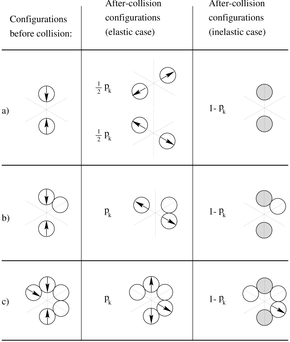
FIG. 1.:

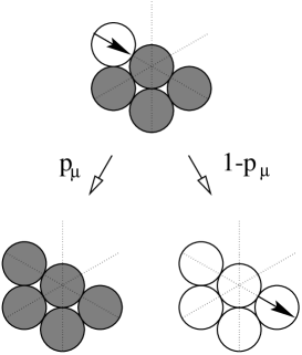
FIG. 2.:

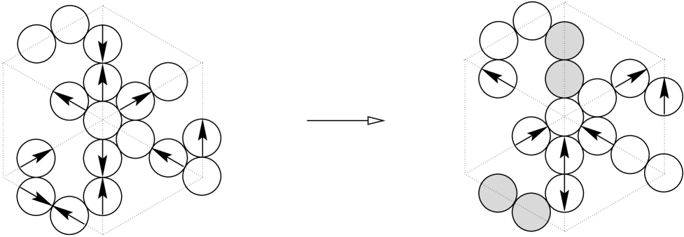
FIG. 3.:

FIG. 4.:

FIG. 5.:

FIG. 6.:

FIG. 7.:

FIG. 8.:

FIG. 9.:

FIG. 10.:

FIG. 11.:

FIG. 12.:

REFERENCES

- [1] P. Bak, C. Tang and K. Wiesenfeld, Phys. Rev. Lett. 59, 381 (1987)
- [2] H.M. Jaeger, C. Liu and S.R. Nagel, Phys. Rev. Lett. 62, 40 (1989)
- [3] G.A. Held et al, Phys. Rev. Lett. 65, 1120 (1990)
- [4] C. Liu, H.M. Jaeger and S.R. Nagel, Phys. Rev. A 43, 7091 (1991)
- [5] M. Bretz et al, Phys. Rev. Lett. 69, 2431 (1992)
- [6] E. Morales, R. Peralta-Fabi and V. Romero-Rochín, Phys. Rev. E 54, 3488 (1996)
- [7] J. Feder, Fractals 3, 431 (1995)
- [8] V. Frette et al, Nature 379, 49 (1996)
- [9] L.A.N. Amaral and K.B.Lauritsen, Physica A 233, 608 (1996); Phys. Rev. E 54, R4512 (1996); cond-mat 9705097 (1997)
- [10] G. Baumann and D.E. Wolf, Phys. Rev. E 54, R4504 (1996)
- [11] U. Frisch, B. Hasslacher and Y. Pomeau, Phys. Rev. Lett. 56, 1505 (1986)
- [12] Lattice Gas Methods for Partial Differential Equations, ed. G.D. Doolen, Addison Wesley (1990)
- [13] H. A. Makse, S. Havlin, P. King and H.E. Stanley, Physica A 233, 587 (1996)
- [14] C.P.C. Prado and Z. Olami, Phys. Rev. A 45, 665 (1992)
- [15] J. Kertész and A. Károlyi, in Proc. of the 6th EPS-APS International Conference on Physics Computing, Lugano, CSCS (1994); A. Károlyi, J. Kertész, in Proc. of the Workshop on Traffic Flow and Granular Materials, Jülich, Eds: D.E. Wolf, M. Schreckenberg and A. Bachem (1996); J. Kertész and A. Károlyi in Proc. of the Third Int. Conf. on Powders & Grains 97, Durham, Eds: R.P. Behringer and J.T. Jenkins (1997)
- [16] G. Peng and H. J. Herrmann, Phys. Rev. E 48, R1796 (1994)
- [17] S. Vollmar and H. J. Herrmann, Physica A 215, 411 (1995)
- [18] J.J. Alonso and H. J. Herrmann, Phys. Rev. Lett. 76, 4911 (1996)
- [19] T. Boutreux and P.G. de Gennes, J. Phys. I 6, 1295 (1996)
- [20] S.S. Manna and J. Kertész, Physica A. 173, 49 (1991)