Brownian Motors driven by Particle Exchange

1 introduction

Directed motion of a Brownian particle can be realized under nonequilibrium conditions. Recently, such Brownian motors have been studied extensively, because they are believed to share common features with biological molecular motors. ${}^{\hbox{\immediate{\bf{?}})}}$ The oldest example of Brownian motors may be Feynmann’s ratchet${}^{\hbox{\immediate{\bf{?}})}}$ which works in contact with two heat baths, while the simplest example may be made by considering time-depending potentials.${}^{\hbox{\immediate{\bf{?}},\penalty 1000\hskip 0.91003pt plus 0.70004pt minus 0.70004pt{\bf{?}},\penalty 1000\hskip 0.91003pt plus 0.70004pt minus 0.70004pt{\bf{?}})}}$ We then find another type of Brownian motors: its non-equilibrium nature is brought about by the existence of two particle reservoirs with different chemical potentials. This type of motors may be most relevant to biological molecular motors. In particular, when we wish to study how chemical energy is converted to mechanical one, we need to have a minimal model to be studied. Until now, some models, in which a chemical reaction is taken into account, have been proposed.${}^{\hbox{\immediate{\bf{?}},\penalty 1000\hskip 0.91003pt plus 0.70004pt minus 0.70004pt{\bf{?}},\penalty 1000\hskip 0.91003pt plus 0.70004pt minus 0.70004pt{\bf{?}})}}$ However, since the models of chemical reactions are assumed without any energetic interpretations, they are not satisfactory to our motivation. We need a model in which energetics associated with particle exchange can be discussed.

The time evolution of a position of a Brownian particle $x$ is assumed to be described by a Langevin equation

$$\gamma{dx\over dt}=-{\partial U\over\partial x}+\xi,$$ (1)

where $\gamma$ is a friction constant, $U(x)$ is a potential function, and $\xi$ is thermal noise satisfying

$$\langle\xi(t)\xi(t^{\prime})\rangle=2\gamma k_{B}T\delta(t-t^{\prime}).$$ (2)

$k_{B}$ is a Boltzmann constant and $T$ denotes temperature. We focus on the regime where inertial effects are negligible. The energetic interpretation of the Langevin dynamics has been presented recently by Sekimoto.${}^{\hbox{\immediate{\bf{?}})}}$ Defining the heat and the work for nonequilibrium processes, he has found the first law of thermodynamics and discussed the energetics for several examples including Feynmann’s ratchet. Subsequently, Sekimoto and Sasa have shown the second law of thermodynamics together with a complementary relation between the irreversible heat and the time lapse.${}^{\hbox{\immediate{\bf{?}})}}$ These results have revealed that the Langevin dynamics is a useful model to discuss energetic aspects of fluctuating systems. We thus wish to extend the Langevin dynamics so that we can discuss the energy transduction caused by particle exchange.

The first step in the present study is to make a mathematical model for equilibrium systems in contact with a particle reservoir. In such systems, grand canonical ensembles should be realized. This is the first necessary condition for the model we wish to have. Until now, two models, in which grand canonical ensembles are realized, have been proposed. One is an extension of the Monte Carlo method,${}^{\hbox{\immediate{\bf{?}})}}$ and the other is designed as a deterministic system${}^{\hbox{\immediate{\bf{?}})}}$ on the same methodology as Nosé invented.${}^{\hbox{\immediate{\bf{?}},\penalty 1000\hskip 0.91003pt plus 0.70004pt minus 0.70004pt{\bf{?}})}}$ However, our concern is not restrict to equilibrium states, but includes non-equilibrium processes. We conjecture that the thermodynamic laws cannot be derived in previously proposed methods. In this paper, we present a model which satisfies two necessary conditions: the realization of grand canonical ensembles at equilibrium and the obedience of the thermodynamic laws for processes between equilibrium states.

This paper is organized as follows. In §2, we study a lattice model and find an evolution rule which realizes grand canonical ensembles. We expect that a continuum limit of the lattice model has a certain relation with the Langevin dynamics in contact with a particle reservoir. In §3, relying on this implicit correspondence between them, we translate the evolution rule on the lattice model to one appropriate to the Langevin dynamics. The validity of our rule is confirmed by numerical simulations. In §4, we derive the thermodynamic relations for processes between equilibrium states. In §5, we devise a model of Brownian motors driven by particle exchange between particle reservoirs. The final section is devoted to discussion.

Before closing this section, we mention a configuration of the system we study. In order to avoid unnecessary complicatedness, we analyze one dimensional systems defined in the region $x>0$. The boundary with a particle reservoir is assumed to be located at $x=0$. Further, interactions among particles are ignored. That is, a potential force acting on each particle is determined by the particle position. In addition, the potential gradient is assumed to vanish at the boundary with the particle reservoir, because we wish to neglect dynamical variables in particle reservoirs. We also assume that the system contacts with a single heat bath of the temperature $T$.

2 lattice model

The lattice we study consists of $M+1$ cites labeled by integers from 0 to $M$. A particle on the $i$-th cite can move to the adjacent cites, the $i+1$-th and the $i-1$-th cite, with the transition probability (per unit time) $w_{i,i+1}$ and $w_{i,i-1}$, respectively. In the Langevin equation eq.(1), the transition probability from $x$ to $x+\Delta x$ during a time interval $\Delta t$ is proportional to${}^{\hbox{\immediate{\bf{?}})}}$

$$\exp(-\gamma\beta{(\Delta x)^{2}\over 4(\Delta t)}-\beta{\Delta U\over 2}),$$ (3)

where $\beta=(k_{B}T)^{-1}$. Since the diffusion expressed in the first term corresponds to a random walk procedure in the lattice model, the simplest form of $w_{ij}$ which has a relation with eq.(3) may be given by

$$w_{ij}=d\exp(-{\beta\over 2}(U_{j}-U_{i}))$$ (4)

for $|i-j|=1$, where $d$ will be related to a diffusion constant. The 0-th cite corresponds to a particle reservoir where the density is kept at constant. We thus assume that $n_{*}$ particles always occupy the 0-th cite irrespective of the transition from/to the 1-st cite, where $n_{*}$ will be related to the particle density in the reservoir. The other cites compose the system in question.

Let us analyze the probability distribution $P(\{n_{i}\},t)$, where $n_{i}$ denotes the particle number on the $i$-th cite. The evolution equation of $P$ is written as${}^{\hbox{\immediate{\bf{?}})}}$

$${\partial\over\partial t}P(\{n_{i}\},t)=\sum_{0\leq i,j\leq M}w_{ij}(\hat{a}_{i}^{\dagger}\hat{a}_{j}-1)n_{i}P(\{n_{i}\},t),$$ (5)

where $n_{0}=n_{*}$, $\hat{a}_{i}^{\dagger}$ and $\hat{a}_{i}$ are creation and annihilation operators of a particle on the $i$-cite, respectively. That is, they are defined as

$$\hat{a}_{i}^{\dagger}f(n_{1},n_{2},\cdots,n_{M}) = f(\cdots,n_{i}+1,\cdots),$$ (6)

$$\hat{a}_{i}f(n_{1},n_{2},\cdots,n_{M}) = f(\cdots,n_{i}-1,\cdots),$$ (7)

and $\hat{a}_{0}^{\dagger}=\hat{a}_{0}=1$. The stationary solution $P_{s}(\{n_{i}\})$ can be obtained in the factorization form

$$P_{s}(\{n_{i}\})=\Pi_{i=1}^{M}{1\over n_{i}!}\exp(-\bar{n}_{i})\bar{n}_{i}^{n_{i}}.$$ (8)

Actually, the substitution of this expression into eq.(5) gives the detailed balance condition

$$w_{i,i+1}\bar{n}_{i}=w_{i+1,i}\bar{n}_{i+1},$$ (9)

where $0\leq i\leq M-1$ and $\bar{n}_{0}=n_{*}$. Solving eq.(9), we obtain

$$\bar{n}_{i}=n_{*}\exp(-\beta(U_{i}-U_{0})).$$ (10)

We then define the chemical potential $\mu$ as

$$\mu=U_{0}+k_{B}T\log n_{*},$$ (11)

by which eq.(8) is rewritten in the form

$$P_{s}(\{n_{i}\})={1\over\Xi}{1\over\Pi_{i=1}^{M}n_{i}!}\exp(\beta(\sum_{i=1}^{M}(\mu-U_{i})n_{i})).$$ (12)

Here, $\Xi$ is a normalization constant called the grand partition function, and calculated as

$$\Xi=\exp(\sum_{i=1}^{M}\exp(\beta(\mu-U_{i}))).$$ (13)

The expression of eq.(12) shows that the particle distribution is given by a grand canonical ensemble with the inverse temperature $\beta$ and the chemical potential $\mu$. We can discuss statistical properties based on eq.(12), for instance, the total number of particles in the system turns out to be poissonian with the average $\bar{N}$, where

$$\bar{N}=\sum_{i=1}^{M}\bar{n}_{i}=\sum_{i=1}^{M}\exp(-\beta(U_{i}-\mu)).$$ (14)

We next derive the rate equation for the particle number on the $i$-cite, $\tilde{n}_{i}(t)$, which is defined as

$$\tilde{n}_{i}(t)=\sum_{\{n_{i}\}}n_{i}P(\{n_{i}\},t).$$ (15)

Multiplying eq.(5) with $n_{i}$ and summing $\{n_{i}\}$, we obtain

$${d\tilde{n}_{i}\over dt} = d\exp(-{\beta\over 2}(U_{i}-U_{i+1}))\tilde{n}_{i+1}$$ (16)

$$+ d\exp(-{\beta\over 2}(U_{i}-U_{i-1}))\tilde{n}_{i-1}$$

$$- d[\exp(-{\beta\over 2}(U_{i+1}-U_{i}))$$

$$+ \exp(-{\beta\over 2}(U_{i-1}-U_{i}))]\tilde{n}_{i}$$

for $1\leq i\leq M-1$, and

$${d\tilde{n}_{M}\over dt} = d\exp(-{\beta\over 2}(U_{M}-U_{M-1}))\tilde{n}_{M-1}$$ (17)

$$- d\exp(-{\beta\over 2}(U_{M-1}-U_{M}))\tilde{n}_{M}.$$

The continuum limit of the expressions of eqs.(16) and (17) will be useful in the argument below. We introduce a lattice spacing $\delta x$ and assume the appropriate scaling of parameters and variables for $\delta x$: $\rho(i\delta x)=\tilde{n}_{i}/\delta x$, $U(i\delta x)=U_{i}$, $x=i\delta x$, $L=M\delta x$, $\rho_{*}=n_{*}/\delta x$, and $d={k_{B}T/\gamma}/(\delta x)^{2}$. Then, the limit $\delta x\rightarrow 0$ provides us

$${\partial\rho\over\partial t}={1\over\gamma}{\partial\over\partial x}({\partial U\over\partial x}+k_{B}T{\partial\over\partial x})\rho,$$ (18)

and the boundary conditions

$$\rho(0,t)=\rho_{*}$$ (19)

at $x=0$ and the density flux vanish at $x=L$. Equation (18) has the same form as the Fokker-Planck equation. However, this is not an evolution equation for the probability distribution, but the rate equation for the particle number distribution. Its actual time evolution fluctuates around a solution to the rate equation.

The stationary solution of eq.(18) under the boundary conditions is derived as

$$\rho_{s}(x)=\rho_{*}\exp(-\beta(U(x)-U(0))),$$ (20)

and the chemical potential becomes

$$\mu=U(0)+k_{B}T\log(\rho_{*}\delta x).$$ (21)

Here, $U(0)$ can be chosen arbitrary because there is no absolute zero in a classical world. Also, $\delta x$ is an unobservable parameter which may be identified to De Broglie length for thermal motion. In the argument below, $U(0)$ and $\delta x$ will be assumed to be arbitrary constants.

3 Langevin Dynamics

In this section, we describe motion of Brownian particles in the physical space $x>0$ which contacts with a particle reservoir at $x=0$. The evolution equation for a particle position is given by eq.(1). We solve this equation numerically by employing a discretization scheme with a time step $\delta t$. The question here is to find a rule related to absorbing and emission from/to the particle reservoir. Since we already know the proper rule for the lattice model, we translate this rule to suitable one for the Langevin dynamics. First, when a particle enters into the region $x\leq 0$, this particle should be interpreted to be absorbed in the particle reservoir. The emission rule is a little bit tactical. Recall that $n_{*}$ particles are always located at the $0$-th cite in the lattice model. Since we wish to make a similar configuration, we assume the following rule: At each time step, a virtual particle is put randomly in the region $-1/\rho_{*}\leq x\leq 0$ and is moved by performing the $\delta t$ integration of eq.(1). Then, if the particle enters into the region $x>0$, this particle should be interpreted to be emitted from the reservoir.

We do not have a mathematical proof that grand canonical ensembles are realized by the rule given here. Nevertheless, we can check its validity by numerical simulations. As a simple example, we assume that an harmonic potential $U=ax^{2}/2$ bounds particles around $x=0$. If our model realizes the grand canonical ensemble with the chemical potential given by eq.(21), a total number of particles $N$ should obey the Poisson distribution:

$$P(N)={1\over N!}\exp(-\bar{N})\bar{N}^{N},$$ (22)

where $\bar{N}$ is calculated as

$$\bar{N}=\rho_{*}\sqrt{\pi k_{B}T\over 2a}.$$ (23)

We performed numerical simulations with parameter values $(a,\gamma,\beta,\rho_{*},\delta t)=(1,1,1,1,0.01)$ and made $P_{num}(N)$, a distribution function of the particle number, by using $10^{4}$ samples every one unit time. We then found that ${\rm sup}_{N}|P(N)-P_{num}(N)|<5\times 10^{-3}$. We also measured how the averaged particle number $\bar{N}_{num}$ depends on the number of samples, $K$. Figure 1 shows that $|\bar{N}_{num}-\bar{N}|$ decreases as $1/\sqrt{K}$, but it has a plateau after $K>5\times 10^{5}$. It comes from the finiteness of $\delta t$. Actually, when $\delta t=0.001$, such a plateau was not observed for $K<10^{6}$. We believe that $\bar{N}_{num}$ approaches to $\bar{N}$ in the limit $\delta t\rightarrow 0$ and $K\rightarrow\infty$. Therefore, we conclude that our evolution rule realizes the grand canonical ensemble with the chemical potential eq.(21).

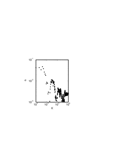
Fig.  1: $\sigma=|\bar{N}_{num}-N|$ versus the number of samples, $K$.

We remark here how the indices of particle positions are assigned in the theoretical analysis developed below. Suppose that there are $N(0)$ particles in the system at $t=0$. Then, a position of the $i$-th particle is denoted by $x_{i}(0)$, $(1\leq i\leq N(0))$, where the ordering is assumed by some rule. When a particle enters to the system first, the particle position is denoted by $x_{N(0)+1}$. Similarly, the unused minimum index is assigned to a position of the new particle. Further, when the $i$-th particle exists in the particle reservoir, $x_{i}=0$ is assumed so as to keep the continuity of $x_{i}(t)$. This convention will be useful, because we do not need to take care whether a particle is in the system or in the reservoir. Instead, we analyze an infinite number of particles.

4 thermodynamics

In this section, we discuss energetics when an external agent changes a parameter $\alpha$ of the potential $U$ during a time interval $[0,\tau]$. Since the external agent should not influence the particle reservoir, we assume that $U(0)$ is kept at constant. The change of the total potential energy in the course of the time evolution is expressed by

$$\Delta U_{tot}=\sum_{i=1}^{\infty}\int_{0}^{\tau}dt\left[{\partial U(x_{i},\alpha)\over\partial x_{i}}{dx_{i}\over dt}+{\partial U(x_{i},\alpha)\over\partial\alpha}{d\alpha\over dt}\right],$$ (24)

where the multiplication has been defined in the Stratonovich sense. By using the evolution equation, the first term is rewritten as

$$Q_{tot}\equiv\sum_{i=1}^{\infty}\int_{0}^{\tau}dt(-\gamma{dx_{i}\over dt}+\xi)\cdot{dx_{i}\over dt}$$ (25)

which can be identified with the energy transfer from the heat bath.${}^{\hbox{\immediate{?})}}$ The second term in eq.(24), denoted by $W$, is interpreted as the work done by the external agent. In this way, for each solution to the Langevin dynamics, we have an energy conservation law

$$\Delta U_{tot}=Q_{tot}+R.$$ (26)

We next discuss the energy transfer between the system and the particle reservoir by assuming

$$\Delta U_{tot} = \Delta U+\Delta U_{R},$$ (27)

$$Q_{tot} = Q+Q_{R},$$ (28)

where the subscript $*_{R}$ denotes the contributions in the reservoir. We do not know the way how to decompose $Q_{tot}$ based on the Langevin dynamics. Instead, we employ the thermodynamic consideration as follows.

$$\Delta U = Q+R+\mu\Delta N,$$ (29)

$$\Delta U_{R} = Q_{R}+\mu\Delta N_{R},$$ (30)

where note that the work cannot be extracted from the particle reservoir because of the equality $\partial U/\partial\alpha=0$ at $x=0$. Then, from the equality

$$\Delta U_{R}=U(0)\Delta N_{R}=-U(0)\Delta N,$$ (31)

we obtain

$$Q_{R}=k_{B}T\log(\rho_{*}\delta x)\Delta N.$$ (32)

This implies that heat associated with particle exchange flows to the particle reservoir. Therefore, the heat transferred to the system from the other all region should be thought as $Q$, not $Q_{tot}$. We will find that such distinction becomes important when we discuss a relation between quasi-static heat and the thermodynamic entropy. (See eqs.(44) and (45).)

Now, we discuss the second law of thermodynamics. In the present case, this is represented by a minimum work principle: the average of $W$ over the possible realizations of paths has a minimum value determined by a thermodynamic potential. In order to prove it, we employ the lattice model again, in which the average of $W$ is given by

$$\langle W\rangle=\int_{0}^{\tau}dt{d\alpha\over dt}\sum_{\{n_{i}\}}\sum_{i=1}^{M}n_{i}{\partial U_{i}\over\partial\alpha}P(\{n_{i}\},t).$$ (33)

Summing $\{n_{i}\}$ first and recalling the definition of $\tilde{n}_{i}(t)$ given by eq.(15), we obtain

$$\langle W\rangle=\int_{0}^{\tau}dt{d\alpha\over dt}\sum_{i=1}^{M}\tilde{n}_{i}(t){\partial U_{i}\over\partial\alpha}.$$ (34)

The continuum limit of this expression becomes

$$\langle W\rangle=\int_{0}^{\tau}dt{d\alpha\over dt}\int_{0}^{\infty}dx\rho(x,t){\partial U(x,\alpha)\over\partial\alpha},$$ (35)

which takes the similar form as the averaged work for the case of one particle Langevin dynamics. Also, as mentioned above, $\rho$ satisfies the Fokker-Planck equation. We thus can develop a similar argument to the previous related study.${}^{\hbox{\immediate{?})}}$ Introducing a stretched time $s=t/\tau$ and the scaled variable $\tilde{\alpha}(t/\tau)=\alpha(t)$, we expand $\rho$ and $\langle W\rangle$ in such a way that

$$\rho = \rho_{0}+{1\over\tau}\rho_{1}+\cdots,$$ (36)

$$\langle W\rangle = \langle W\rangle_{0}+{1\over\tau}\langle W\rangle_{1}+\cdots,$$ (37)

where we have assumed that $1/\tau$ is a small parameter. We then solve eq.(18) perturbatically. At the lowest order, we obtain

$$\rho_{0}(x,s)=\rho_{*}\exp(-\beta(U(x,\tilde{\alpha}(s))-U(0))),$$ (38)

and this yields

$$\langle W\rangle_{0} = \int_{0}^{1}ds{d\tilde{\alpha}(s)\over ds}\int_{0}^{\infty}dx\rho_{0}(x,s){\partial U(x,\tilde{\alpha})\over\partial\tilde{\alpha}},$$ (39)

$$= -k_{B}T[\bar{N}(\tilde{\alpha}(1))-\bar{N}(\tilde{\alpha}(0))].$$ (40)

Here, from eqs.(13) and (14), the grand potential defined by $\Omega=-k_{B}T\log\Xi$ is calculated as $-k_{B}T\bar{N}$. As the result, the quasi-static work turns out to be equivalent to the increment of the grand potential, that is,

$$\langle W\rangle_{0}=\Delta\Omega.$$ (41)

Therefore, in the quasi-static limit, eq.(29) becomes

$$\Delta\bar{U}=\langle Q\rangle_{0}+\Delta\Omega+\mu\Delta\bar{N},$$ (42)

where $\bar{U}$ and $\bar{N}$ are the energy and the particle number averaged over the equilibrium ensemble for a given value of $\tilde{\alpha}$. Then, when we define the entropy through a thermodynamic relation of the grand potential

$$\Omega=\bar{U}-TS-\mu\bar{N},$$ (43)

we recover a standard relation:

$$\langle Q\rangle_{0}=T\Delta S.$$ (44)

Substituting eqs.(32) and (44) to eq.(28), we also obtain

$$\langle Q_{tot}\rangle_{0}=T\Delta S+k_{B}T\log(\rho_{*}\delta x)\Delta\bar{N}.$$ (45)

Kitahara has proposed a similar expression in the context of the work efficiency for heat engines in open systems.${}^{\hbox{\immediate{\bf{?}})}}$

At the next order in the perturbative expansion, we obtain

$$\hat{L}\rho_{1}=-{\partial\rho_{0}\over\partial s},$$ (46)

where the operator $\hat{L}$ is given by

$$\hat{L}=-{1\over\gamma}{\partial\over\partial x}\left[{\partial U\over\partial x}+k_{B}T{\partial\over\partial x}\right].$$ (47)

In order to solve eq.(46) under the boundary condition $\rho_{1}(0)=0$, we introduce a Green function defined by

$$\hat{L}(\rho_{0}(x)g(x,y))=\delta(x-y),$$ (48)

where $g(x,y)=g(y,x)$ and $g(0,y)=0$. Such a Green function exists owing to the Hermiteness of the operator $\hat{L}(\rho_{0}\cdot)$ defined under the given boundary condition. Also, since we focus on the case that a stable stationary distribution is realized, all eigenvalues of $\hat{L}$ are expected to be non-negative, and this leads that $g(x,y)$ is a semi-positive definite in the sense that

$$\int_{0}^{\infty}dx\int_{0}^{\infty}dyg(x,y)\phi_{1}(x)\phi_{2}(y)\geq 0,$$ (49)

where $\phi_{1}$ and $\phi_{2}$ are arbitrary functions in a certain functional space. Using the Green function $g(x,y)$, we express $\rho_{1}(x)$ as

$$\rho_{1}(x)=[-\int_{0}^{\infty}dyg(x,y){\partial\rho_{0}\over\partial s}]\rho_{0}(x).$$ (50)

This yields the first order contribution to the non-static work:

$$\langle W\rangle_{1} = \int_{0}^{1}ds\left({d\tilde{\alpha}(s)\over ds}\right)^{2}\int_{0}^{\infty}dx\int_{0}^{\infty}dy$$ (51)

$${\partial U(x,\tilde{\alpha})\over\partial\tilde{\alpha}}g(x,y){\partial U(y,\tilde{\alpha})\over\partial\tilde{\alpha}}\rho_{0}(x)\rho_{0}(y).$$

We then find that $\langle W\rangle_{1}$ is non-negative due to eq.(49). Therefore, the minimum work principle

$$\langle W\rangle\geq\langle W\rangle_{0}=\Delta\Omega$$ (52)

holds within the validity of the perturbation theory. In the similar way as developed in the previous study,${}^{\hbox{\immediate{?})}}$ we can also derive a complementary relation between the excess work and the time lapse.

5 Brownian Motor

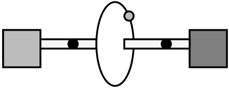
Fig.  2: Schematic figure of a model of Brownian motors driven by particle exchange.

Fig.  3: Averaged time evolution of the motor angle $\phi$. The graph was created by averaging $10^{4}$ samples of $\phi(t)$ with $t=0.01\times i$, where $1\leq i\leq 1000$.

As an application of the Langevin dynamics in contact with a particle reservoir, we present a simple model of Brownian motors driven by particle exchange. The system is assumed to be in the region $-L/2\leq x\leq L/2$ and to contact with particle reservoirs at $x=\pm L/2$. The density in the particle reservoirs are denoted by $\rho_{+}$ and $\rho_{-}$, respectively. A motor particle is confined in a circle whose center is located at $x=0$. (See Fig. 2.) We assume that time evolution of the angle of motor angle $\phi$ is described by a Langevin equation with a friction constant $\gamma_{\phi}$. The form of the potential function of the system can be chosen rather arbitrarily. We found however that we need fine tuning of the model so that we can confirm the motor behavior numerically. In this paper, we report the result of the model

$$U(\{x_{i}\},\phi)=\sum_{i=1}^{\infty}A(x_{i})\eta(\phi-\phi_{0}(x_{i})),$$ (53)

where

$$A(r)=\left\{\begin{array}[]{lr}b&|r|\leq r_{0},\\ b({(r-r_{0})^{2}\over(r_{1}-r_{0})^{2}}-1)^{2}&r_{0}\leq|r|\leq r_{1},\\ 0&|r|\geq r_{1},\end{array}\right.$$ (54)

$$\phi_{0}(r)=\left\{\begin{array}[]{lr}{\pi\over 2}\left[\left({r\over r_{0}}\right)^{3}-3{r\over r_{0}}\right]&|r|\leq r_{0},\\ -\pi{\rm sign}(r)&|r|\geq r_{0},\end{array}\right.$$ (55)

and

$$\eta(\phi)=\sin(\phi)+1.$$ (56)

Notice that the form of $U(\{x_{i}\},\phi)$ has been assumed so that the motor angle turns around when a particle moves slowly from one end to the other end. In numerical simulations, we fix the values of the following parameters as $L=1$, $\gamma=1$, $\gamma_{p}=0.01$, $b=0.25$, $r_{0}=0.3$, $r_{1}=0.4$, and $\delta t=10^{-4}$, and regard $\rho_{+}$, $\rho_{-}$ and $k_{B}T$ as control parameters. The chemical potential difference is then given by

$$\delta\mu=\mu_{+}-\mu_{-}=k_{B}T\log({\rho_{+}\over\rho_{-}}).$$ (57)

Under the equilibrium condition $\delta\mu=0$, directed motion never occur. We confirmed that the averaged time evolution of $\phi$ tends to be constant as the number of samples increases. On the other hand, when $\delta\mu\neq 0$, the motor rotates in one direction on the average. In Fig. 3, we showed the averaged time evolution of $\phi$ for the parameter values: $(\rho_{+},\rho_{-})=(2.0,0.04)$ and $k_{B}T=0.1$. This shows the clear evidence of directed motion. We now discuss a quantitative aspect a little bit. In particular, we are concerned with a ratio of the frequency of the motor rotation with the particle number current at $x=0$, which is denoted by $Y$. Recalling the form of the potential function, one may conjecture that $Y$ is closed to one. We found however that $Y$ sharply depends on the choice of the parameter value. As one example, in Fig. 4, $Y$ was plotted against $k_{B}T$. $Y$ decreases quickly for the increment of the temperature. We do not understand the reason yet. Detailed study is in progress and will be reported elsewhere.

Fig.  4: Ratio of the motor frequency with particle number current, denoted by $Y$, versus $k_{B}T$.

6 discussion

We address a few comments. Our stochastic model for particle reservoirs seems reasonable, but its validity is not confirmed completely. The correspondence between the lattice model and the Langevin dynamics still remains at an intuitive level. We expect that a mathematical proof will be presented. In numerical simulations, we have studied cases that there is no interaction among particles. We believe that our model goes well even if the interaction is included, because properties of particle reservoirs should not depend on the choice of systems.

We do not understand the nature of Brownian motors so much. For example, the work efficiency for Feynmann ratchet was shown to be much less than Carnot efficiency,${}^{\hbox{\immediate{?})}}$ on the contrary to the Feynmann’s stimulating insight.${}^{\hbox{\immediate{?})}}$ The efficiency will be discussed in our motor model, but this will be much less than a value allowed by thermodynamics.${}^{\hbox{\immediate{\bf{?}})}}$ Elaborate study on energy transduction along the time axis is necessary to clarify the peculiarity of Brownian motor.

The relevance to biological molecular machines may be most stimulating. Based on the present study, we wish to consider chemical kinetics, enzyme catalysis, and biological membranes.

References

- [1] R. D. Astumian: Science 276 (1997) 917.
- [2] R. P. Feynmann, R. B. Leighton and M. Sands: The Feynmann Lectures on Physics, (Addison-Wesley, Reading, 1963) Vol. I.
- [3] M. O. Magnasco: Phys. Rev. Lett. 71 (1993) 1477.
- [4] R. D. Astumian and M. Bier: Phys. Rev. Lett. 72(1994) 1766.
- [5] J. Prost, J. F. Chauwin, L. Peliti, and A. Ajari: Phys. Rev. Lett. 72 (1993) 2652.
- [6] M. O. Magnasco: Phys. Rev. Lett. 72 (1994) 2656.
- [7] R. D. Astumian and M. Bier: Biophys. J. 70 (1996) 637.
- [8] H.X. Zhou and Y. D. Chen: Phys. Rev. Lett. 77 (1996) 194.
- [9] K. Sekimoto: J. Phys. Soc. Jpn. 66, (1997) 1234.
- [10] K. Sekimoto and S. Sasa: J. Phys. Soc. Jpn. to be published in No.11, 66, (1997).
- [11] D. J. Adams: Mol. Phys.28 (1974) 1241; Mol. Phys.29 (1974) 307.
- [12] T. Çagin and B. M. Pettitt: Molecular Simulation 6 (1991) 5.
- [13] S. Nosé : J. Chem. Phys. 81 (1984) 51; Mol. Phys. 52 (1984) 255.
- [14] W. G. Hoover, Phys. Rev. A 31 (1985) 1695.
- [15] H. Risken: The Fokker-Plank Equation (Springer-Verlag, Berlin, 1989). See also L. Onsarger and S. Machlup: Phys. Rev. 91 (1951) 1509; N. Hashizume: J. Phys. Soc. Jpn. 8, (1952) 461.
- [16] N.G. Van Kampen: Stochastic Processes in Physics and Chemistry (North-Holland, 1992).
- [17] K. Kitahara: private communication.
- [18] The efficiency of chemical engines should be discussed carefully. See T. Shibata and S. Sasa: preprint, ’equilibrium chemical engines’ submitted to J.Phys.Soc. Jpn.