N. Rajewsky, L. Santen, A. Schadschneider and

M. Schreckenberg

Abstract     The asymmetric exclusion process (ASEP) has attracted a lot of interest not only because its many applications, e.g. in the context of the kinetics of biopolymerization and traffic flow theory, but also because it is a paradigmatic model for nonequilibrium systems. Here we study the ASEP for different types of updates, namely random-sequential, sequential, sublattice-parallel and parallel. In order to compare the effects of the different update procedures on the properties of the stationary state, we use large-scale Monte Carlo simulations and analytical methods, especially the so-called matrix-product Ansatz (MPA). We present in detail the exact solution for the model with sublattice-parallel and sequential updates using the MPA. For the case of parallel update, which is important for applications like traffic flow theory, we determine the phase diagram, the current, and density profiles based on Monte Carlo simulations. We furthermore suggest a MPA for that case and derive the corresponding matrix algebra.
Key Words: Asymmetric exclusion process; boundary-induced phase transitions; steady state; matrix product Ansatz; discrete-time updates

1 Introduction

For nonequilibrium systems in low dimensions an understanding can often be gained by studying rather simple models [1, 2, 3, 4, 5, 6]. The one-dimensional asymmetric exclusion process (ASEP) has been used to describe various problems in different fields of interest, such as the kinetics of biopolymerization [7] and traffic [8]. On the other hand, the ASEP is so simple that it has achieved a paradigmatic status for nonequilibrium systems [9]. It can be mapped onto a surface growth model known as the single-step model [10] and in the appropriate hydrodynamical limit its density profile obeys the Burgers equation which is itself closely related to the KPZ equation [11]. The ASEP can also be viewed as a prototype for so-called boundary-induced phase transitions [12]: the boundaries, which can inject and remove particles from the system, govern – in a subtle interplay with the local dynamical rules – the macroscopic behaviour of the model and can produce different phases and phase transitions.

In [13] recursion relations on the system size have been derived for the ASEP with random-sequential update and open boundary conditions. Open boundaries here and in the following mean that particles are injected at one end of a chain of $L$ sites with probability $\alpha$ and are removed at the other end with probability $\beta$. In [13] these recursion relations were solved for the special case $\alpha=\beta=1$. This solution was later extended in [14] to general $\alpha$ and $\beta$. A very elegant solution of the general case was given at the same time in [15] using a matrix product Ansatz (MPA) for the weights of the stationary configurations similar to the matrix product groundstate of certain quantum spin chains [16]. This Ansatz can be used to compute density profiles and correlation functions. The relationship between the MPA for quantum spin chains and one-dimensional models of statistical physics will be discussed in this paper.

Since then the MPA was extended to find the transient of the model [17], to describe the ASEP with a defect in form of an additional particle with a different hopping rate [18] or a blockage [19], to solve the case of oppositely charged particles (with hard-core repulsion), which move in opposite directions (driven by an external electric field) and can interchange their charge if they meet [20]. The MPA was also used to recover solutions of certain integrable reaction-diffusion models [21].

Most of these solutions have been found for random-sequential dynamics. In that case the master equation can be rewritten as a Schrödinger-like equation for a “Hamiltonian” with interactions between nearest-neighbours only [22]. Other updates lead to more complicated master equations with non-local interactions.

It also turned out that the MPA is not just an Ansatz. The stationary state of an one-dimensional stochastic model with arbitrary nearest-neighbor interactions and random-sequential update can always be written as a matrix product [23]. This is also true for an ordered-sequential or sublattice-parallel update, which can be shown to be intimately related [24]. The matrices in the MPA are generally infinite-dimensional. Therefore, evaluating physical quantities such as density profiles is still a formidable task, but often it is at least possible to obtain asymptotic expressions. However, in certain regions of the parameter space the matrices can reduce to low-dimensional variables. A simple example is the case of one-dimensional matrices, which is equivalent to a mean-field solution.

The implementation of the order of application of the local transition rates for a given model (the type of update) is an essential part of the definition of the model, since the transient and even the stationary state may differ dramatically [25]. In the following, the ASEP will be studied with types of update that are often more useful for Monte Carlo simulations than the random-sequential update. The aim of this paper is to use the ASEP as a case study to investigate the consequences of different types of updates onto the stationary state of a nonequilibrium model with open boundaries. Concerning the analytical treatment, the MPA turns out to be a useful tool.

Hinrichsen [26] was the first to apply the MPA to the ASEP with sublattice-parallel update and deterministic bulk dynamics. He could confirm earlier conjectures for the correlation functions [27]. It is important to note that this update is substantially different from the fully-parallel update used for example for modeling traffic flow. Nevertheless, to our knowledge this is the first model with a discrete-time update which has been solved using the MPA. The results presented here build partially on our previous work [28], where we found a mapping of the ASEP with ordered-sequential and sublattice-parallel update onto the random-sequential case. For sublattice-parallel update this was done independently by Honecker and Peschel [29]. We will explain the mapping in more detail and give a physical interpretation of the underlying Ansatz. As a by-product, we solve the model on a ring.

We also study numerically and analytically the ASEP with parallel update and present new results like the phase diagram and the current. We show that the model can be described by a matrix-product structure at least for small systems. The underlying algebra is somewhat different to the other ones because a third state appears, which is neccessary to decompose the transfer matrix into a more simple product.

This paper is organized as follows: Section 2 gives the definitions of the model and the updates used and establishes a precise relationship between the MPA for the stationary state of a stochastic model and for the groundstate of quantum spin chains. Section 3 is devoted to the MPA for the ASEP with discrete-time updates. In Section 3.1 the matrix algebra for the ordered-sequential and the sublattice-parallel update is derived. In Section 3.2 we propose a MPA for the parallel update by mapping the model onto a 3-state model with an ordered-sequential update. Furthermore, we find a special line in parameter space where the 2-cluster approximation becomes exact. In Section 4 we use the mathematical results of Section 3 and Monte Carlo simulations to calculate the current, density profiles and correlation functions for the discrete-time updates. Finally, Section 5 contains a concluding discussion. We have included several appendices, which mainly list details of the calculations.

2 Definition of the ASEP and the MPA

2.1 The ASEP and the different updates

Consider sites located on a chain of length $L$. Each site $i$ ($1\leq i\leq L$) is either occupied by a particle ($\tau_{i}=1$), or it is empty ($\tau_{i}=0$). We have three basic mechanisms (see Fig. 1): Hopping: We look at the pair $(i,i+1)$. If we find a particle at site $i$ and no particle (“hole”) at site $i+1$, we move the particle one site to the right with probability $p$. In the remaining cases, nothing happens.
Injection and removal: At the boundaries particles/holes can be injected and/or removed. At the left boundary a particle can be injected with probability $\alpha$ if site $1$ is empty. At the right end of the chain a particle will be removed with probability $\beta$.
The model can be generalized to allow hopping in both directions by introducing a probability $q$ for hopping onto an unoccupied site to the left. Furthermore, one can also inject particles at the right end and remove particles at the left end. These modifications do not change the basic features of the model and will not be considered in the following.

We now have to define the order in which to perform the hopping, the injection and the removal in terms of time and space. There are four basic ways to do that:
(a) random-sequential update: We pick at random a site $i$. If $2\leq i\leq L-1$, each particle has a probability $pdt$ of jumping to the right (if this site is empty). If $i=1$ , we allow for hopping to the right with probability $pdt$ and particle injection with rate $\alpha$ if this site is empty. For $i=L$ a particle is removed with rate $\beta$ if the site is occupied. This update is the realization of the usual master equation in continuous time. A different $p$ would simply result in a rescaling of time (see Sect. 3). As a consequence, the phase diagram of the ASEP with update (a) depends only trivially on $p$. Therefore one can set $p=1$ which is most efficient for computer simulations.
The following three updates are discrete in time.
(b) sublattice-parallel update: We first use our rule for injection (removal) at site $1$($L$). We then perform our rules for hopping on the pairs $(2,3)$,$(4,5)$ etc. After that, we update the pairs $(1,2)$,$(3,4)$ etc ($L$ has to be even). This update can be used efficiently for computer simulations. Its main advantage for theoretical purposes is that its transfer matrix can be written as a product of local terms.
(c) ordered-sequential update: We start at the right end of the chain and remove a particle at site $i=L$ with probability $\beta$. We then update the pair $(i=L-1,i=L)$. We continue with pair $(i=L-2,i=L-1)$ and so forth, until the left end of the chain is reached. After the update of pair $(i=1,i=2)$, we allow for injection at site $i=1$. For models where particles only hop to the right this update may also be called more precisely ’backward-ordered-sequential update’.
Obviously, the order of update can also be reversed. For the ASEP, these two updates are connected by a particle-hole symmetry: injecting particles can be regarded as removing holes, and vice versa. Therefore it is sufficient to study just one of the ordered-sequential updates.
We would like to point out that in principle one has to distinguish two different types of ordered-sequential updates which one could name site-ordered-sequential and particle-ordered-sequential, respectively. In contrast to the site-ordered-sequential update described in (c) above, in the particle-ordered-sequential update the rules are only applied to occupied sites, i.e. to particles. This might have a strong effect, as can be seen most easily for the case of small particle numbers and the completely asymmetric deterministic case $p=1$. In the case of site-sequential update a single particle injected at the left end moves through the lattice in one timestep (i.e., one sweep through the lattice). For the particle-sequential update a timestep means updating occupied sites only and so the particle moves only one site. By looking at a lattice with two particles, one can already see that the two different updates might introduce rather different correlations. Starting with particles separated by $d$ empty sites, in the site-ordered-sequential update the left particle will move to the right until it reaches the right particle, which then starts to move. On the other hand, in the case of particle-ordered-sequential update the particles will stay always $d$ or $d-1$ sites apart. For general values of $p$ the situation is similar.
The differences between these two sequential update procedures manifest itself also in the solution for periodic boundary conditions. We will come back to this point in Section 4.1. In the following we will always consider the site-ordered-sequential update – until stated otherwise – to which we will refer as ordered-sequential update for brevity.
(d) parallel update: The rules for hopping, injection, and removal are applied simultaneously to all sites of the whole chain.
The parallel update usually produces the strongest correlations and is used for traffic simulations [8]. In the case of the ASEP, it is nearly identical to the particle-ordered-sequential update.

Fig. 2 illustrates the updates (b) and (c).

If the ASEP with updates (a)-(c) is put on a ring (no injection/removing of particles and periodic boundary conditions), a trivial stationary state (where correlations are absent, see below) is reached, while update (d) produces a particle-hole attraction [36]. This already shows that different updates might yield a different behaviour.

For analytic calculations usually the random-sequential update is most convenient since it can be formulated in terms of a “Hamiltonian” with nearest-neighbour interaction. In Monte Carlo simulations, however, ordered-sequential updates can be implemented more effectively.

At this point it is necessary to point out the existence of some confusion in the nomenclature of the different updates. The random-sequential update (a) is sometimes simply called ’sequential update’, as is the ordered-sequential one. In several publications the sublattice-parallel update (b) is called ’parallel’ which makes it necessary to refer to the parallel update (d) as ’fully-parallel’. We urge the reader to check carefully which type of update is actually used when consulting the literature. In order to avoid further confusion we will use the terminology which seems to us the most precise.

2.2 Master equation and quantum formalism

Our starting point is the master equation for an arbitrary one-dimensional stochastic process. Following [22] we rewrite this equation as a Schrödinger-like equation in imaginary time. We consider a chain of $L$ sites $j$ with state variables $\tau_{j}=0,1$. Generalizations to the case where the state variables can take more than two values are straightforward. A configuration of the whole system will be denoted by $\{\tau\}=\{\tau_{1},\tau_{2},...,\tau_{L}\}$, its weight by $P(\{\tau\},t)$.

The master equation then has the form

$$\frac{\partial}{\partial t}P(\{\tau\},t)=\sum_{\{\tau^{\prime}\}}\left[w(\tau^{\prime}\rightarrow\tau)P(\{\tau^{\prime}\},t)-w(\tau\rightarrow\tau^{\prime})P(\{\tau\},t)\right]$$ (1)

where $w(\tau\rightarrow\tau^{\prime})$ denotes the rate for a transition from $\{\tau\}$ to $\{\tau^{\prime}\}$.
Let us now define a ket state $|P(t)\rangle$ in the following way. We take an orthonormal basis in the configuration space $\{\tau\}$,

$$|\tau\rangle=|\tau_{1},...,\tau_{L}\rangle$$ (2)

with $\langle\tau^{\prime}|\tau\rangle=\delta_{\tau^{\prime},\tau}$ and define

$$|P(t)\rangle=\sum_{\{\tau\}}P(\{\tau\},t)|\tau\rangle\,,$$ (3)

i.e. we have $P(\{\tau\},t)=\langle\tau|P(t)\rangle$. It is then easy to see that

$$\frac{\partial}{\partial t}|P(t)\rangle=-{\cal H}\,|P(t)\rangle$$ (4)

holds, with the (generally non-hermitean) “Hamiltonian” ${\cal H}$ given by

$$\langle\tau|{\cal H}|\tau^{\prime}\rangle=-w(\tau^{\prime}\rightarrow\tau)$$ (5)

for the off-diagonal elements ($\tau\neq\tau^{\prime}$) and by

$$\langle\tau|{\cal H}|\tau\rangle=\sum_{\{\tau\}\neq\{\tau^{\prime}\}}w(\tau\rightarrow\tau^{\prime})$$ (6)

for the diagonal elements.
From (4) one can see that the stationary state $|P_{0}\rangle$ of the stochastic model corresponds to the “groundstate” with ”groundstate energy” zero ($E_{0}=0$) of the ”quantum spin chain” defined by (5), (6), i.e.

$${\cal H}|P_{0}\rangle=0.$$ (7)

The conditions (5), (6) guarantee that the real parts of the other eigenvalues $E_{\lambda}$ of ${\cal H}$ are non-negative. Using the bra groundstate $\langle 0|=\sum_{\{\tau\}}\langle\tau|$, the average of an observable ${\cal A}(\{\tau\})$ at time $t$ is given by

$$\langle{\cal A}\rangle(t)=\sum_{\{\tau\}}{\cal A}(\{\tau\})P(\{\tau\},t)=\langle 0|{\cal A}|P(t)\rangle.$$ (8)

Expanding the initial state $|P(t=0)\rangle=\sum_{\lambda}a_{\lambda}|\psi_{\lambda}\rangle$ in terms of the eigenkets $|\psi_{\lambda}\rangle$ with eigenvalues $E_{\lambda}$ of ${\cal H}$ this can be rewritten as

$$\langle{\cal A}\rangle(t)=\langle 0|{\cal A}|P(t)\rangle=\langle 0|{\cal A}e^{-{\cal H}t}|P(t=0)\rangle=\sum_{\lambda}a_{\lambda}e^{-E_{\lambda}t}\langle 0|{\cal A}|\psi_{\lambda}\rangle.$$ (9)

This shows that the behaviour for large times $t$ is governed by the low-lying excitations.
We now restrict ourselves to stochastic processes with random-sequential dynamics and local and homogenous transition rates $\Gamma_{\tau_{j}\tau_{j+1}}^{\tau^{\prime}_{j}\tau^{\prime}_{j+1}}$ (denoting the rate for a local transition of sites $j$ and $j+1$ from (${\tau^{\prime}_{j}\tau^{\prime}_{j+1}}$) to (${\tau_{j}\tau_{j+1}}$)), which do not depend on time. In this case ${\cal H}$ is a sum of local Hamiltonians with nearest-neighbour interaction only [22]:

$${\cal H}=\sum_{j=1}^{L}h_{j}\quad\,$$ (10)

with

$$h_{j}=\begin{pmatrix}\Gamma_{01}^{00}+\Gamma_{10}^{00}+\Gamma_{11}^{00}&-\Gamma_{00}^{01}&-\Gamma_{00}^{10}&-\Gamma_{00}^{11}\\ -\Gamma_{01}^{00}&\Gamma_{00}^{01}+\Gamma_{10}^{01}+\Gamma_{11}^{01}&-\Gamma_{01}^{10}&-\Gamma_{01}^{11}\\ -\Gamma_{10}^{00}&-\Gamma_{10}^{01}&\Gamma_{00}^{10}+\Gamma_{01}^{10}+\Gamma_{11}^{10}&-\Gamma_{10}^{11}\\ -\Gamma_{11}^{00}&-\Gamma_{11}^{01}&-\Gamma_{11}^{10}&\Gamma_{00}^{11}+\Gamma_{01}^{01}+\Gamma_{10}^{11}\end{pmatrix}$$ (11)

(the basis is $(00)$,$(01)$,$(10)$,$(11)$). Each column of $h_{j}$ adds up to $0$, because the probability has to be conserved.
For the updates (b)-(d) it is generally not possible to write ${\cal H}$ in the form (10) since one would have to include terms acting on sites which are not neighboured. It is then more suitable to use directly the transfer matrix $T$ describing the update of the whole chain during one timestep. In the case of the ordered-sequential update, $T$ is simply a product of the local transfer matrices $t_{j}=h_{j}-1$. It follows

$$|P(t+1)\rangle=T|P(t)\rangle,$$ (12)

which means that in order to find the stationary state, one has to solve for the eigenvector of $T$ with eigenvalue $1$.

2.3 Optimum groundstates and MPA for quantum spin chains

The construction of optimum ground states for quantum spin chains via matrix products was introduced in [16] (see also [31, 30] and [32] for further references). Let us consider a Hamiltonian for a quantum spin chain (with periodic boundary conditions) of the form ${\cal H}^{\prime}\,=\,\sum_{j=1}^{L}h_{j}^{\prime},$ where $h_{j}^{\prime}$ is the local hermitian Hamiltonian and independent of $j$, acting only on spin $j$ and $j+1$.
It is always possible to set the lowest eigenvalue of $h_{j}^{\prime}$ equal to zero by adding a suitable constant. Then $h_{j}^{\prime}$ is positive-semidefinite and since ${\cal H}^{\prime}$ is the sum of positive-semidefinite operators, it follows that zero is a lower bound for the ground state energy $E_{0}$ of ${\cal H}^{\prime}$, i.e. $E_{0}\geq 0$. Usually, $E_{0}$ is greater than zero ($E_{0}>0$) and the global groundstate involves also excited states of $h_{j}^{\prime}$. Therefore, a construction of the global groundstate is usually very difficult.
However, there are special cases where $E_{0}$ is equal to zero,

$${\cal H}^{\prime}|\psi_{0}\rangle\,=\,0$$ (13)

and therefore for all $j$

$$h_{j}^{\prime}\,|\psi_{0}\rangle\,=\,0.$$ (14)

A state $|\psi_{0}\rangle$ is called optimum groundstate of ${\cal H}^{\prime}$ if and only if condition (14) holds. This implies that the groundstate energy is independent of the system size, i.e. there are no finite-size corrections.
The idea is now to construct groundstates by means of a product of matrices,

$$|\psi_{0}\rangle\,=\,{\rm Tr}\,(m_{1}\otimes m_{2}\otimes...\otimes m_{L})\,,$$ (15)

where the entries of matrix $m_{j}$ are spin-1 single-site states and the symbol $\otimes$ denotes the usual matrix multiplication of matrices with a tensor product of the matrix elements. Note that $m_{1}\otimes m_{2}\otimes...\otimes m_{L}$ is still of the same size as the matrices $m_{j}$, but its elements are large linear combinations of tensor product states. The trace assures the translation invariance of the groundstate. For non-periodic boundary conditions it has to be replaced by a suitable linear combination of the elements of $m_{1}\otimes m_{2}\otimes...\otimes m_{L}$.
As an example [16], the ground state of a large class of antiferomagnetic spin-1 chains can be constructed using the $S^{z}$ eigenstates $|0\rangle_{j}$ and $|\pm\rangle_{j}$ by

$$m_{j}=\begin{pmatrix}a\,|0\rangle_{j}&b\,|+\rangle_{j}\\ c\,|-\rangle_{j}&d\,|0\rangle_{j}\end{pmatrix}\,,$$ (16)

where the $a,b,c,d$ are real numbers. Condition (14) requires

$$h_{j}^{\prime}\,(m_{j}\otimes m_{j+1})\,=\,0\quad,$$ (17)

i.e. all four elements of $m_{j}\otimes m_{j+1}$ are local groundstates of $h_{j}$. Let us now write

$$m_{j}=A_{0}\cdot|0\rangle+A_{-}\cdot|-\rangle+A_{+}\cdot|+\rangle\,$$ (18)

with suitable $2\times 2$ matrices $A_{0}$ and $A_{\pm}$. The ’$\cdot$’ denotes a product of each entry of the matrix to the left with the single-site state on the right.
It is obvious that (15) can be written equivalently as

$$|\psi_{0}\rangle={\rm Tr}\bigg{[}\bigg{(}\begin{array}[]{c}A_{0}\\ A_{-}\\ A_{+}\end{array}\bigg{)}\otimes\bigg{(}\begin{array}[]{c}A_{0}\\ A_{-}\\ A_{+}\end{array}\bigg{)}\otimes...\otimes\bigg{(}\begin{array}[]{c}A_{0}\\ A_{-}\\ A_{+}\end{array}\bigg{)}\bigg{]}\,,$$ (19)

or, defining a column vector

$$A\,=\,\bigg{(}\begin{array}[]{c}A_{0}\\ A_{-}\\ A_{+}\end{array}\bigg{)}\quad,$$ (20)

as

$$|\psi_{0}\rangle={\rm Tr}(A\otimes A\otimes...\otimes A)\quad.$$ (21)

The condition (17) then be rewritten as

$$h_{j}^{\prime}\,(A\otimes A)\,=\,0\quad.$$ (22)

This means that there are two equivalent ways to write $|\psi_{0}\rangle$. While (15) uses a product of matrices with vectors as entries (the usual notation for quantum spin chains), (21) expresses $|\psi_{0}\rangle$ as a product of vectors with matrices as entries. The original idea of Derrida et.al. [15] was to construct the stationary state $|P_{0}\rangle$ of a stochastic process defined by (10) as a suitable linear form of a product of matrices where each matrix corresponds to a single-site state precisely as in (21).

2.4 MPA for stochastic systems

In the following we want to describe how the MPA can be applied to stationary states $|P_{0}\rangle$ of stochastic systems. In contrast to the case of quantum spin chains we already know the corresponding “groundstate energy” of the stochastic Hamiltonian ${\cal H}$ defined by (5) and (6). From (4) we see that ${\cal H}|P_{0}\rangle=0$ and therefore the groundstate energy is zero, independent of the system size. This hints at the applicability of the MPA and a possible generalization of the optimum groundstate concept.

Indeed it turns out that, using an MPA of the form (21), (14) can be replaced by a more general condition by allowing for a divergence-like term [21], i.e.

$$h_{j}(A\otimes A)={\bar{A}}\otimes A-A\otimes{\bar{A}}\ ,$$ (23)

where the vector $\bar{A}$ can be different from the vector $A$. It is easy to see that (for periodic boundary conditions) the divergence-like terms cancel after summing over $j$. Hence, the stationary state of the stochastic process described by (5) and (6) is of the form (21).

For hermitian Hamiltonians one always has $\bar{A}=A$ and (23) reduces to (22). Therefore one can regard (23) as the generalization of the optimum groundstate concept to non-hermitian Hamiltonians.

Again it is possible to generalize these ideas to treat non-periodic boundary conditions. As an example we briefly review the solution of the ASEP with random-sequential update and open boundary conditions. The “Hamiltonian” reads (hopping rate $p$, feeding and removal rates $\alpha$,$\beta$):

$$H={\bar{h}_{1}}+{\bar{h}_{L}}+\sum_{j=1}^{L-1}h_{j}$$ (24)

with the boundary terms

$${\bar{h}_{1}}=\begin{pmatrix}\alpha&0\\ -\alpha&0\\ \end{pmatrix}\ ,\qquad{\bar{h}_{L}}=\begin{pmatrix}0&-\beta\\ 0&\beta\\ \end{pmatrix}$$ (25)

and the bulk “Hamiltonian”

$$h_{j}=\begin{pmatrix}0&0&0&0\\ 0&0&-p&0\\ 0&0&p&0\\ 0&0&0&0\end{pmatrix}\quad.$$ (26)

From (9) we can see that $p$ only rescales time (and $\alpha$ and $\beta$) and that it would therefore be sufficient to study $p=1$.

Following the MPA, the matrix for the particle (hole) is denoted by $D$ ($E$), so that $A=\left(\begin{array}[]{c}E\\ D\end{array}\right)$. Since the ASEP with open boundary conditions has (in general) no translational invariance, the trace in (21) is replaced with a scalar product:

$$|P_{0}\rangle=\frac{1}{Z_{L}}\langle\langle W|A\otimes\cdots\otimes A|V\rangle\rangle\,,$$ (27)

where the normalization constant $Z_{L}$ is equal to $Z_{L}=\langle W|C^{L}|V\rangle$ with $C=E+D$. The brackets $\langle\langle...\rangle\rangle$ indicate that the scalar product is taken in each entry of the vector $A\otimes...\otimes A$.
More explicitly (27) means that the weight $P(\tau_{1},\ldots,\tau_{L})$ of a configuration $\{\tau\}$ in the stationary state is given by

$$P(\tau_{1},\ldots,\tau_{L})=\frac{1}{Z_{L}}\langle W|\prod_{j=1}^{L}\left[\tau_{j}D+(1-\tau_{j})E\right]|V\rangle.$$ (28)

Thus one has a simple recipe for the calculation of the (unnormalized) weight of an arbitrary configuration $\{\tau\}$: Translate the configuration into a product of matrices by identifying an empty site ($\tau_{j}=0$) with $E$ and an occupied site ($\tau_{j}=1$) with $D$. For example, the configuration $011001\cdots$ corresponds to the product $EDDEED\cdots=ED^{2}E^{2}D\cdots$. Then multiply by the vectors $\langle w|$, $|v\rangle$ from the left and right, respectively.

We assume that $\bar{A}$ in (23) is of the form $\bar{A}=\left(\begin{array}[]{c}\bar{E}\\ \bar{D}\end{array}\right)$ where $\bar{E}$ and $\bar{D}$ denote matrices acting in the same vectorspace as $E$ and $D$. Executing the sum (10) in (23) leads to a cancelation of all terms in the bulk of the chain. The remaining terms at the boundaries vanish if the vectors $\langle W|$ and $|V\rangle$ are chosen appropriately:

$$\langle W|{\bar{h}_{1}}A=-\langle W|{\bar{A}}\quad,\quad{\bar{h}_{L}}A|V\rangle={\bar{A}}|V\rangle\,.$$ (29)

Inserting (25) and (26) into (23), (29) we get a system of quadratic equations in $E,D,{\bar{E}}$ and ${\bar{D}}$ which is called the algebra of Ansatz (23). The dimension of the matrices is not determined by the Ansatz. However, taking ${\bar{E}}=\mathbf{1}=-{\bar{D}}$, the equations reduce to the “DEHP algebra” [15]

$$p\,DE = D+E\quad,$$ (30)

$$\alpha\langle W|E = \langle W|\quad,$$ (31)

$$\beta D|V\rangle = |V\rangle\quad.$$ (32)

Equation (30) can be guessed intuitively: the current $J_{L}(j)$ (describing the flux of particles through bond $j$ of a chain of length $L$) has to be constant throughout the chain. $J_{L}(j)$ is given by [15]

$$J_{L}(j)=\frac{p}{Z_{L}}\langle W|C^{j-1}DEC^{L-j-1}|V\rangle\quad,$$ (33)

and we see that $DE\propto C=E+D$ is the simplest way to achieve a constant current.
It is possible to derive explicit expressions for $D$, $E$, $\langle W|$ and $|V\rangle$ [15]. It turns out, that one finds one-dimensional representations if and only if

$$\alpha+\beta=p.$$ (34)

In all the other cases, the matrices are infinite-dimensional.
Up to this point, the MPA appears to be just an Ansatz for the stationary state. However, it can be shown [23] that the MPA (27) with the “cancellation-mechanism” (23) is an equivalent reformulation of the master equation for a stochastic process with random-sequential update and nearest-neighbour interaction. Therefore it is of general interest to study the quadratic algebras which are produced by (23) and to try to find explicit representations [33, 35, 34].
In the next section, we will construct the stationary state for the ASEP with sequential and sublattice parallel update. Note that we do not have a “Hamiltonian” of the form (10) in this case and that the “cancellation mechanism” will not be appropriate.

3 MPA for the ASEP with updates in discrete time

In this section we will generalize the results for the random-sequential update to discrete-time updates. In Section 3.1 we solve the ASEP for sublattice-parallel and sequential updates using the MPA. In Section 3.2 we conjecture a MPA for the parallel update.

Let us briefly discuss the precise connection between the random-sequential update and the ordered-sequential update, say from the right to the left, for an arbitray one-dimensional stochastic process with nearest neighbor interaction. We have seen, that in this case the ”Hamiltonian” describing the random-sequential dynamics is of the form (10), ${\cal H}=\sum_{j=1}^{L}h_{j}$, while for the ordered-sequential udpate one has to use the transfer matrix

$$T=\prod_{j=1}^{L}t_{j}$$ (35)

with local matrices $t_{j}$ connecting the sites $j$ and $j+1$. From (10) and (9) it is clear that one of the parameters can be used to rescale the time unit; in the case of the ASEP this leads to expressions which are independent of the hopping probability $p$. For the update (35) with discrete time, this is obviously impossible and we expect the phase diagram of the ASEP to depend on $p$ nontrivially. Only in the limit of vanishing densities these two updates can be mapped onto each other [29] by inserting $t_{j}=h_{j}-\mathbf{1}$ (where $\mathbf{1}$ denotes the identity matrix) into (35) and expanding the product. For nonvanishing densities, the equations (10) and (35) are connected nontrivially via additional, non-locals terms.

3.1 Sublattice-parallel and ordered-sequential update

We now solve the ASEP with ordered-sequential (update (c)) and sublattice-parallel (update (b)) dynamics. So far, the ASEP with the latter update and deterministic hopping has been studied by Schütz [27] and Hinrichsen [26]. A brief account of our work has been given in [28]. For simplicity, we will first concentrate on the ordered-sequential update (c) from the right to the left. Since this update is discrete in time, a stochastic “Hamiltonian” of the form (10) is not at hand. Therefore, the transfer matrix $T_{\leftarrow}$ has to be used. This means by definition

$$|P(t+1)\rangle\,=\,T_{\leftarrow}|P(t)\rangle$$ (36)

The stationary state $|P_{0}\rangle$ must not change under the action of the $T_{\leftarrow}$ and therefore is eigenvector with eigenvalue $1$ of $T_{\leftarrow}$:

$$|P_{0}\rangle\,=\,T_{\leftarrow}|P_{0}\rangle\,.$$ (37)

Let us now explicitly write down $T_{\leftarrow}$. The boundary conditions can be represented by operators ${\cal R}$ and ${\cal L}$ acting on site $j=L$ and $j=1$, respectively:

$${\cal R}\;=\;\left(\begin{array}[]{cc}1&\beta\\ 0&1-\beta\end{array}\right)\,,\hskip 28.45274pt{\cal L}\;=\;\left(\begin{array}[]{cc}1-\alpha&0\\ \alpha&1\end{array}\right)\,.$$ (38)

The basis chosen for ${\cal R}$ and ${\cal L}$ is $(0,1)$. The update-rule for any pair of sites $(j,j+1)$ can be written as

$${\cal T}_{j}\;=\;\left(\begin{array}[]{cccc}1&0&0&0\\ 0&1&p&0\\ 0&0&1-p&0\\ 0&0&0&1\end{array}\right)\,.$$ (39)

The basis is $(00,01,10,11)$, and we have

$$T_{\leftarrow}=L\cdot T_{1}\cdot...\cdot T_{L-1}\cdot R$$ (40)

with

$$L = {\cal L}\otimes\mathbf{1}\otimes...\otimes\mathbf{1}\,,$$

$$R = \mathbf{1}\otimes...\otimes\mathbf{1}\otimes{\cal R}\,,$$ (41)

$$T_{j} = \mathbf{1}\otimes\mathbf{1}...\otimes{\cal T}_{j}\otimes\mathbf{1}...\otimes\mathbf{1}\,,$$

where $\mathbf{1}$ denotes the identity matrix.
Formally, a “Hamiltonian” can be defined as ${\cal H}_{\leftarrow}=\mathbf{1}-T_{\leftarrow}$. However, ${\cal H}_{\leftarrow}$ cannot be written simply as a sum of local “Hamiltonians”. This means that while we can try a MPG Ansatz (27) we cannot use the “cancellation”-mechanism (23).
However, the sequential nature of $T_{\leftarrow}$ suggests another mechanism:

$${\cal T}\,\left[A\otimes\hat{A}\right]\;=\;\hat{A}\otimes A\,,$$ (42)

$$\langle W|{\cal L}\hat{A}\;=\;\langle W|A\,,\hskip 42.67912pt{\cal R}A|V\rangle\;=\;\hat{A}|V\rangle\,,$$ (43)

where $\hat{A}=\left(\begin{array}[]{c}\hat{E}\\ \hat{D}\end{array}\right)$ with square matrices $\hat{E},\hat{D}$.
This means that a “defect” $\hat{A}$ – corresponding to a local perturbation of the stationary state defined by (37) – is created in the beginning of an update at site $j=L$, which is then transported through the chain, until it reaches the left end and disappears.
Equation (42) leads to the following bulk algebra:

$$[E,\hat{E}]=[D,\hat{D}] = 0,$$

$$E\hat{D}+pD\hat{E} = \hat{E}D,$$ (44)

$$(1-p)D\hat{E} = \hat{D}E,$$

and the boundary conditions

$$\begin{array}[]{c}\langle W|\hat{E}(1-\alpha)\;=\;\langle W|E\,,\\[2.84526pt] \langle W|(\alpha\hat{E}+\hat{D})\;=\;\langle W|D\,,\end{array}\hskip 5.69054pt\begin{array}[]{c}(1-\beta)D|V\rangle\;=\;\hat{D}|V\rangle,\\[2.84526pt] (E+\beta D)|V\rangle\;=\;\hat{E}|V\rangle.\end{array}$$ (45)

The ordered-sequential update in the opposite direction (left to right) can be treated in the same way. The stationary state is given by

$$|P_{0}\rangle_{\rightarrow}=\frac{1}{Z_{L}}\langle\langle W|\hat{A}\otimes\cdots\otimes\hat{A}|V\rangle\rangle$$ (46)

with the same mechanism (42) and (43). However, it is more convenient to use the particle-hole symmetry for the calculation of averages.

For completeness let us briefly discuss the sublattice-parallel update (b). In this case the transfer matrix has the structure [26, 29]

$$T_{s-\parallel}=T_{1}\cdot T_{2}$$ (47)

with

$$T_{1} = {\cal L}\otimes{\cal T}\otimes{\cal T}\cdots\otimes{\cal T}\otimes{\cal R},$$

$$T_{2} = \phantom{{\cal L}}{\cal T}\otimes{\cal T}\cdots\otimes{\cal T}\otimes{\cal T},$$ (48)

and the MPA for the stationary state is of the form

$$|P_{0}\rangle_{s-\parallel}=\frac{1}{Z_{L}}\langle\langle W|\hat{A}\otimes A\otimes\hat{A}\otimes A\cdots\otimes\hat{A}\otimes A|V\rangle\rangle.$$ (49)

One can now use exactly the same mechanism (42), (43) as in the ordered-sequential case and thus obtains the same algebra (3.1), (45). For $p=1$ the algebra was first derived and solved by Hinrichsen [26] using a two-dimensional representation for $E$, $D$, $\hat{E}$, $\hat{D}$, $\langle W|$, $|V\rangle$.

The fact that the ordered-sequential and the sublattice-parallel update lead to the same algebra (3.1), (45) implies the existence of an intimate relationship between the averages of observables. Although the stationary states themselves are different, they are connected via transformations, and it can be shown that the density profile of the ordered-sequential update from the left (right) to the right (left) corresponds to the density of the even (odd) sites produced by the sublattice-parallel update [24]. This result holds for arbitrary stochastic models with nearest neighbor interactions.
One can check that for

$$(1-\alpha)(1-\beta)=1-p\quad,$$ (50)

a one-dimensional solution of the algebra exists. This equation defines a line in the phase diagram where the mean-field solution becomes exact. It turns out that this line touches all phases. This makes it possible to calculate quantitites such as the current very easily, because the analytic expression for the current does not change inside a phase.

For general values of $\alpha$, $\beta$ and $p$ the algebra (3.1) and (45) can be mapped onto the generalized DEHP-algebra [28]. This is shown in App. A and will be used later in Section 4.2. App. B discusses the consequences of the particle-hole symmetry for the two ordered-sequential updates in more detail. App. C deals with the special case of symmetric diffusion.

3.2 Parallel update

As far as analytic approaches are concerned, this update poses the greatest difficulties, since it produces the strongest correlations. In the case of the ASEP, this becomes obvious when looking at the model put on ring: All updates, except the parallel [36] and particle-sequential [37] one, lead to a trivial state where correlations are absent. In the case of the parallel update, it is known [36] that a particle-hole attraction appears: the probability to find an empty site in front of an occupied site is enhanced compared to the mean-field result.
The model with parallel update and periodic boundary conditions has first been solved exactly in [36, 8] using a cluster approximation (see below). Here the weights are decomposed into products of pairs of sites overlapping just one site. It turned out that this 2-cluster approximation becomes exact for periodic boundary conditions.
We now make an analogous calculation for the model with open boundary conditions. The goal is to find the parameter set for which the density profile is flat. Note that a flat density profile does not necessarily mean that there are no correlations between the sites. We denote the probability for the pair configuration $\tau_{i}\tau_{i+1}$ at site $i,i+1$ by $P_{\tau_{i}\tau_{i+1}}$($\tau_{i}=1,0$ and $i=1,...,L$). Let us assume that such a probability for a certain pair configuration is independent of the position of the pair. The condition $P_{01}=P_{10}$ leads to a flat density profile ($\langle\tau_{1}\rangle=\langle\tau_{2}\rangle=...=\langle\tau_{L}\rangle$), but $P_{\tau_{i}\tau_{i+1}}$ is not necessarily equal to $P_{\tau_{i}}\cdot P_{\tau_{i+1}}$.
The 2-cluster approximation corresponds to a factorization of the weight $P(\tau_{1},\tau_{2},...,\tau_{L})$:

$$P(\tau_{1},\tau_{2},...,\tau_{L})=R_{\tau_{1}}\cdot P_{\tau_{1}\tau_{2}}\cdot P_{\tau_{2}\tau_{3}}\cdot...\cdot P_{\tau_{L-1}\tau_{L}}\cdot R_{\tau_{L}}\quad,$$ (51)

where the $R$’s reflect the influence of the boundaries; they can be set to $R_{0}=1$ and $R_{1}=r$.
It is sufficient to study a system of 3 sites. The generalization to larger systems is straightforward [36].
The (exact) master equation for the stationary state reads $x=Tx$ where $x$ is a vector containing the 8 possible configurations, and $T$ is the $8\times 8$-dimensional transfer matrix for $L=3$. By inserting Ansatz (51) into this master equation it is straightforward to show that (51) is exact if and only if

$$(1-\alpha)(1-\beta)=1-p.$$ (52)

This means that the condition we have found for a constant density profile is exactly the same as for the other discrete-time updates, see (50). The reason for this coincidence is still unkown. Note that (52) is not a simple mean-field line.

In the following we will propose a MPA for the parallel update. (51) suggests that matrices denoting pairs of particles and/or holes should be used. The main problem is that the resulting algebra will be very complex, since it will contain many variables (matrices). On the other hand, if we use a MPA of the form (27), a simple mean-field solution will not be found, e.g. there will be no scalar solution for the algebra. However, such an Ansatz could produce (51) under condition (52) in the form of a low-dimensional representation.
Furthermore, even if a choice for the MPG is made, we still have to find a mechanism which ensures stationarity. The transfer matrix, however, cannot be decomposed easily in products or sums of local terms.
The main difference between the parallel update and the ordered-sequential update from the left to the right is that in the parallel update, a particle can move only one site to the right (per update of the chain). This enables us to use the ordered-sequential update, if we introduce a third state for particles that have been moved. The local (sequential) update operator then has to transform a third-state particle into a “normal” particle in the following update step.
We write down the Ansatz

$$|P_{0}\rangle\;=\;{Z_{L}}^{-1}\;\langle W|\,\left(\begin{array}[]{c}E\\[-2.84526pt] D\end{array}\right)^{\otimes L}|V\rangle\,\,,$$ (53)

which has to satisfy

$$T_{\parallel}\,|P_{0}\rangle=|P_{0}\rangle\quad.$$ (54)

The update-rule ${\cal T}$ for any pair of sites $(i,i+1)$ is now nine-dimensional. However, since the third state must not appear after the update, the last four rows and every third column are irrelevant (here set to zero). The explicit expression for ${\cal T}$ can be found in Appendix E. We have

$$T_{\parallel}=R\cdot T_{L-1}\cdot...\cdot T_{1}\cdot L$$ (55)

with

$$L = {\cal L}\otimes\mathbf{1}\otimes...\otimes\mathbf{1}\,,$$

$$R = \mathbf{1}\otimes...\otimes\mathbf{1}\otimes{\cal R}\,,$$ (56)

$$T_{i} = \mathbf{1}\otimes\mathbf{1}...\otimes{\cal T}_{i}\otimes\mathbf{1}...\otimes\mathbf{1}\,.$$

The mechanism for stationarity reads now

$${\cal T}\,\left[\Biggl{(}\begin{array}[]{c}\hat{E}\\[-2.84526pt] \hat{D}\\[-2.84526pt] \hat{F}\end{array}\Biggr{)}\otimes\Biggl{(}\begin{array}[]{c}E\\[-2.84526pt] D\\[-2.84526pt] 0\end{array}\Biggr{)}\right]\;=\;\Biggl{(}\begin{array}[]{c}E\\[-2.84526pt] D\\[-2.84526pt] 0\end{array}\Biggr{)}\otimes\Biggl{(}\begin{array}[]{c}\hat{E}\\[-2.84526pt] \hat{D}\\[-2.84526pt] \hat{F}\end{array}\Biggr{)}\,,$$ (57)

$$\langle W|{\cal L}\Biggl{(}\begin{array}[]{c}E\\[-2.84526pt] D\\[-2.84526pt] 0\end{array}\Biggr{)}\;=\;\langle W|\Biggl{(}\begin{array}[]{c}\hat{E}\\[-2.84526pt] \hat{D}\\[-2.84526pt] \hat{F}\end{array}\Biggr{)}\,,\hskip 42.67912pt{\cal R}\Biggl{(}\begin{array}[]{c}\hat{E}\\[-2.84526pt] \hat{D}\\[-2.84526pt] \hat{F}\end{array}\Biggr{)}|V\rangle\;=\;\Biggl{(}\begin{array}[]{c}E\\[-2.84526pt] D\\[-2.84526pt] 0\end{array}\Biggr{)}|V\rangle\,,$$

with the new third-state matrix $\hat{F}$. This leads to an algebra, which can be found in Appendix F. Note that the last bulk equation $0=D\hat{F}$ excludes a scalar solution for the algebra. This is consistent with our earlier observation that there is no simple mean-field solution of the model.
First, we can check the relations which connect the densities at the ends of the chain with the current $J$. This calculation can be done for arbitrary system sizes and is presented in Appendix G.
Second, it is possible to show that the algebra correctly describes a system of three sites. This can be done by taking the expressions for the weights of the eight possible configurations of the stationary state given by (54) and by applying several times the algebraic rules. Thereby each weight can be expressed as a linear combination of the other weights. The resulting system of linear equations turns out to be identical to those obtained from the transfer matrix $T$.
Thirdly, it can be checked whether the algebra can be reduced to a generalized DEHP-algebra of the type

$$p\,D\,E=a\,E+b\,D$$ (58)

with some numbers $a,b$. This equation induces certain relations between weights for a system of size $L$ and $L-1$, which can be checked using the exact solutions. It turned out that (58) cannot be valid.
We found a two-dimensional representation for the bulk algebra [38], but despite intensive effort, we could not solve the complete algebra. Therefore, Monte Carlo simulations have been performed [39]. The results will be presented in Section 4.2.

4 Comparative study of physical quantities

In the following we will investigate the consequences of the mathematical description developed in the previous section. First we investigate the ASEP with periodic boundary conditions for the different updates. This will allow us later to distinguish between “pure” bulk effects and “boundary-induced” bulk effects. After that we will derive and compare the phase diagrams, density profiles and other physical quantities for the various updates.

4.1 Periodic boundary conditions

For random-sequential dynamics the stationary state of the ASEP with periodic boundary conditions is given by $|P_{0}\rangle=\frac{1}{Z_{L}}{\rm Tr}(A\otimes\dots\otimes A)$ where the elements $E$ and $D$ of the vector $A$ satisfy the algebra (30) and the normalization is given by $Z_{L}={\rm Tr\,}C^{L}$ with $C=E+D$. Since the boundary equations (31) and (32) do not have to be considered, it is possible to find a one-dimensional representation of the matrices $E$ and $D$ which then become real numbers $e$, $d$. The current is calculated from $J_{L}=\frac{p}{Z_{L}}{\rm Tr}(C^{j-1}DEC^{L-j-1})=\frac{1}{c}$, where we have used (30) and $Z_{L}=c^{L}$ with $c=e+d$. In contrast to the case of open boundary conditions, the density $\rho$ is now fixed and the density profile is constant, $\rho=\langle\tau_{j}\rangle$, independent of $j$. With

$$\langle\tau_{j}\rangle=\frac{1}{Z_{L}}{\rm Tr}(C^{j-1}DC^{L-j})$$ (59)

one finds $\rho=d/c$. Therefore the current is given by

$$J(\rho,p)=p\rho(1-\rho)\,.$$ (60)

This is exactly the mean-field result, because in mean-field approximation a site is occupied with probability $\rho$ and its right neighbour is empty with probability $1-\rho$. Since hopping then occurs with probability $p$, one obtains (60).
This result is not surprising as the existence of a one-dimensional representation implies the absence of correlations between neighbouring sites, i.e. the MPA reduces to mean-field theory.

We now turn to the ASEP with backward-sequential update on a ring. The state

$$|P_{0}\rangle\;=\;\frac{1}{Z_{L}}{\rm Tr}\bigl{[}A^{\otimes(L-1)}\otimes\hat{A}\bigr{]}$$ (61)

is obviously translation-invariant and, because of (42), stationary (the argument of the trace is a vector with a product of matrices in each component; the trace has to be applied to each component). The algebra can be directly solved with one-dimensional matrices (see Appendix D). The current $J_{\leftarrow}(\rho,p)$ for the ordered-sequential update is not given by (33), but by

$$J_{\leftarrow}(j)=\frac{p}{Z_{L}}\langle W|C^{j-1}D\hat{E}C^{L-j-1}|V\rangle\quad.$$ (62)

For the case of periodic boundary conditions one finds

$$J_{\leftarrow}(\rho,p)=p\rho\frac{1-\rho}{1-p\rho}.$$ (63)

Fig. 3 illustrates this result. Again this result can be obtained directly using a mean-field argument. The site to the right of an occupied site is empty with probability $1-(\rho-J_{\leftarrow})$. Here one has to take into account that the density is reduced by $J_{\leftarrow}$ after the update of that site. Therefore the current satisfies $J_{\leftarrow}=p\rho(1-(\rho-J_{\leftarrow}))$ which leads to (63). The maximal flow ($p$ fixed) is reached for a density $\rho^{\rm max}_{\leftarrow}(p)=\frac{1}{p}(1-\sqrt{1-p})\geq 1/2$. The sequential update $T_{\leftarrow}$ “likes” high $p$ and high densities. The particle-hole symmetry can be used to determine these quantities for $T_{\rightarrow}$ simply by replacing $\rho$ with $1-\rho$: $T_{\rightarrow}$ “prefers” high $p$ and low densities.
It is interesting to compare (63) with the well-known result [36] for parallel update,

$$J_{\parallel}(\rho,p)=\frac{1}{2}\biggl{(}1-\sqrt{1-4p\rho(1-\rho)}\biggr{)}.$$ (64)

For the parallel update a mean-field theory for the distances between consecutive particles becomes exact [40]. Similar results have been obtained recently by Evans [37], who solved the ASEP with periodic boundary conditions in the presence of disorder with parallel update and a particle-sequential update by generalizing the approach of [31].
$J_{\parallel}(\rho,p)$ is obviously symmetrical with respect to $\rho=1/2$. It is maximal at $\rho_{\parallel}^{\rm max}=1/2$ for all values of $p$, while $\rho_{\leftarrow}^{\rm max}$ is always higher than $1/2$ (except for $p=0$).
Hence, the maximal currents (for a given $p$) are $J_{\leftarrow}(\rho^{\rm max},p)=\frac{2}{p}(1-\sqrt{1-p})-1$ and $J_{\parallel}(\rho^{\rm max},p)=\frac{1}{2}(1-\sqrt{1-p})$. It is intuitively clear that $J_{\leftarrow}(\rho^{\rm max},p)>J_{\parallel}(\rho^{\rm max},p)$ holds, and it can be verified easily.

Let us now return to the model with open boundary conditions.

4.2 Phase diagram

The phase diagram for random-sequential dynamics has been determined for $p=1$ in [13, 15, 14]. This is no restriction since, as mentioned before, $p$ only rescales time (and $\alpha\to\alpha/p$, $\beta\to\beta/p$). Since it will turn out that the phase diagrams for the different updates are rather similar we will not repeat the results for the random-sequential update here. Instead we will first determine the phase diagram for the ASEP with open boundary conditions and discrete time by using the results of Section 3.1 and discuss the differences to the random-sequential case later. In Appendix A it is shown how the algebra (3.1),(45) can be projected onto the DEHP-algebra. The representations of this algebra (and the resulting phase diagram) are known for all parameter values $\alpha,\beta,p,q$ [43, 33, 34]. Therefore, we have obtained explicit expressions for the matrices and vectors, and have thus constructed the stationary state of our model; we do not have to be concerned about representations any more that might not satisfy (A) since the projection onto the DEHP-algebra already covers the whole parameter space.
Furthermore, it is straightforward to calculate observables such as the current and the density, at least in principle.
The mapping of App. A strongly suggests that the well-known phase diagram of the ASEP with random-sequential update and stochastic hopping in both directions [43, 33, 34] will also be valid for the ASEP with ordered-sequential update. This is indeed correct and has been proven directly in [29]. The phase diagram is shown in Fig. 4. The mean-field line is the curved dashed line. Also shown are density profiles calculated from Monte Carlo simulations. All well-known features of the phase diagram (high-density phase, low-density phase, maximum current phase, coexistence line with linear density profile) are recovered. The intersection of the mean-field line (50) with the line $\alpha=\beta$ defines the endpoint $\alpha_{c}$ (=$\beta_{c}$) of the coexistence line. This yields

$$\alpha_{c}\,=\,1-\sqrt{1-p}.$$ (65)

In the case of deterministic hopping ($p=1$), the maximum current phase vanishes, and we recover the result of Hinrichsen [26].
It is known that for the DEHP-algebra, the mean-field expressions for the current are exact. Since the mean-field line touches all three phases, we can calculate the corresponding currents and bulk densities for our model. Our results are

$$J(\alpha,\beta,p)=\begin{cases}\frac{\alpha}{p}\frac{p-\alpha}{1-\alpha}&\text{in the low-density phase},\\ \frac{\beta}{p}\frac{p-\beta}{1-\beta}&\text{in the high-density phase},\\ \frac{1-\sqrt{1-p}}{1+\sqrt{1-p}}&\text{in the maximum current phase},\end{cases}$$ (66)

which is in excellent agreement with our numerical data.
Since the relation $J(\alpha,\beta,p)=\beta\rho(\alpha,\beta,p,x=L)$ is exact, we immediately get the bulk density in the high-density phase: $\rho_{\rm bulk}=\frac{1}{p}\frac{p-\beta}{1-\beta}$. The bulk density in the low-density phase will be obtained below. Fig. 5 shows a space-time diagram for a point on the coexistence line ($p=0.75,\alpha=\beta=0.3$) produced by the Monte Carlo simulation. The well-known fluctuating shock can nicely be observed.
Typical space-time diagrams for the different phases can be found in Fig. 6. The “jams” in the high-density phase move from the right to the left. In the low-density phase, groups of particles (small jams) move from the left to the right.

For the case of parallel dynamics extensive Monte Carlo simulations have been performed [39] which revealed that the phase diagram looks essentially the same as before (Fig. 4). Again, we find a high- (low-) density and a maximum current phase and a linear density profile along the line $\alpha=\beta$, until the 2-cluster line (52) is touched.
Since we have a particle-hole symmetry in the model, the density for $\alpha=\beta$ and odd lattice sizes has to be $1/2$ for site $\frac{L+1}{2}$. Therefore, the ’bulk density’ $\rho(\alpha,\beta,p,x=\frac{L+1}{2})$ in the maximum current phase must be $1/2$.
Equations (51) and (52) can be used to calculate the current

$$J(\alpha,\beta,p)=\begin{cases}{\alpha}\frac{p-\alpha}{p-{\alpha}^{2}}&\text{in the low-density phase},\\ \beta\frac{p-\beta}{p-{\beta}^{2}}&\text{in the high-density phase},\\ \frac{1-\sqrt{1-p}}{2}&\text{in the maximum current phase},\end{cases}$$ (67)

and the remaining bulk densities $\rho_{\rm bulk}=\frac{\alpha(1-\alpha)}{p-{\alpha}^{2}}$ (low-density) and $\rho_{\rm bulk}=\frac{p-\beta}{p-{\beta}^{2}}$ (high-density phase). These results are exact on the 2-cluster line (52). For general values of $\alpha$ and $\beta$ we find an excellent agreement with the numerical data. Fig. 6 presents typical space-time diagrams in the various phases. The particle-hole attraction is apparent.

Note that for every update the maximal current $J(\rho^{\rm max},p)$ on the ring (as calculated in Section 4.1) is equal to the value of the current in the maximum current phase for that update. The value of $\rho^{\rm max}$ gives the corresponding bulk density. This shows that the current in the maximum current phase is determined by the ’capacity’ of the ring.

4.3 Density profiles and phase transitions

For the parallel update we performed extensive Monte Carlo simulations in order to determine quantities like density profiles and correlation functions. In this section we will compare these results with those obtained analytically and numerically for the other update types.

The results presented in Section 4.2 show that one can distinguish at least three different phases with respect to the flow. In the low- (high-) density phase the current depends for a given value of $p$ only on $\alpha$ ($\beta$) and in the maximum current phase the current is independent of the chosen in- and output rates. This basic structure of the phase diagram is the same for all types of update although the bulk properties change drastically.

A more detailed analysis of ASEP with random-sequential update has shown [14] that the system is governed by two independent length scales $\xi_{\alpha}$ and $\xi_{\beta}$, which represent the influence of the boundaries. At the critical value of $\alpha$ and $\beta$ these length scales diverge and a phase transition occurs. This divergence produces two additional phases compared to the mean-field results. Thus the parameter space is divided into five different phases. The low-density phases AI and AII, where the bulk properties are determined by the value of $\alpha$, the high-density phases BI and BII, where the output rate $\beta$ determines the flow, and the maximum current phase where the flow is independent of $\alpha$ and $\beta$. The phases AI and AII (BI and BII) are distinguished by the behaviour of the density profile near the boundaries (see below).

We checked this scenario for the parallel and ordered-sequential update. In order to avoid difficulties due to the $p$-dependent scale factor of the phase diagram we analyzed the density profiles for $p=0.75$. Our simulation results are obtained for systems with $320$ sites. Since finite-size corrections are rather small, this size is already sufficient to obtain the behaviour in the limit of large $L$.

We first measured the density profile in the low-density phases AI and AII. In [14, 15] it has been shown that for large $L$ the asymptotic behaviour near the boundaries changes from a pure exponential decay in the phase AI to the enhanced exponential decay according to $\exp(-(L-x)/\xi_{\alpha})/\sqrt{L-x}$ in the phase AII. This change of the behaviour near the boundaries is due to the divergence of the length scale $\xi_{\beta}$ at the transition line. $\xi_{\beta}$ remains infinite throughout the whole phase AII. Unfortunately, the divergence of $\xi_{\beta}$ cannot be calculated directly because the relevant length scale $\xi$, which determines the exponential decay in AI, is given by

$$\xi^{-1}=\bigl{|}\xi_{\alpha}^{-1}-\xi_{\beta}^{-1}\bigr{|}.$$ (68)

Thus the correlation length $\xi$ remains finite at the transition line from AI to AII. In contrast to the divergence of $\xi_{\beta}$, the asymptotics of the density profile can be checked against the numerical results. Fig. 7 shows that the density profile for $\alpha=0.40$, $\beta=0.42$ and parallel update can be nicely fitted by a pure exponential decay, but within the phase AII the enhanced exponential form has to be used (see also the insert in Fig. 4). Another characteristic line crossing the low-density phase AII is the mean-field line, where the density profile is completely flat. This line separates the monotonously decreasing density profiles from monotonously increasing profiles, but the asymptotic behaviour is left unchanged. The behaviour of the density profiles in the high-density phases BI and BII can be obtained using the particle symmetry of the model.

The transition between the high- and low-density phases is driven by the diverging length scale $\xi$. This divergence occurs although both length scales are finite, because at the transition line $\xi_{\alpha}$ and $\xi_{\beta}$ coincide. The qualitative agreement of the density profile strongly suggest that the relevant length scale in the low-density phase is given by (68) also for discrete-time updates. Moreover, the comparison of the numerically estimated correlation length shows that the correlation lengths of the parallel and ordered-sequential update are identical and differ from those obtained for the random-sequential only by a constant factor (Fig. 8). Exactly at the transition line $\alpha=\beta$, one finds a linear density profile as shown in Fig. 9. This linear profile is result of a fluctuating shock front which separates for a given time a high-density region from a low-density region. The position of the shock front fluctuates through the whole lattice such that a time average over all single time profiles gives a linear profile.

The transition from the low- (high-) density phase AII (BII) to the maximum current phase is characterized by a change of the asymptotic behaviour of the density profile from the enhanced exponential to a pure algebraic decay. The transition is driven by the divergence of the length scale $\xi_{\alpha}$ ($\xi_{\beta}$) for $\alpha\rightarrow\alpha_{c}$ ($\beta\rightarrow\beta_{c}$). Both length scales are infinite not only at the transition line but for all values of $\alpha$ and $\beta$ larger than the critical value. Therefore an algebraic decay of the density profile can be observed in the whole maximum current phase. Fig. 10 shows the diverging correlation length for different update types. Again the length scales of the updates with discrete time agree and the length scales produced by the random-sequential update are larger if one considers the same in- and output rates.

The flow is generated by the (10)-clusters (the mobile pairs), while the other 2-cluster configurations exclude hopping of particles. Therefore, we measured density profiles of the probabilities $P_{\tau_{i}\tau_{i+1}}$ of 2-cluster configurations $\tau_{i}\tau_{i+1}$. One gets a flat profile of the mobile pairs $P_{1_{i}0_{i+1}}$ (see Fig. 11) which is a consequence of eq. (33) for the current in the case of parallel dynamics. The nontrivial part of the density profile is produced by the immobile pairs. The identity $P_{1_{i}0_{i+1}}=P_{0_{i}1_{i+1}}$, which is already known from the periodic system [8], is only true for flat density profiles. One observes qualitatively the same behaviour for the random-sequential, but not for the ordered-sequential update.
For the ordered-sequential update the transport of a local defect changes the behaviour of the $P_{\tau_{i}\tau_{i+1}}$ profiles: The density of particles in front of hole at the defect site (in the case of backward-sequential update) determines the flow and therefore none of the 2-cluster configurations is in general translation-invariant after a sweep through the lattice.

5 Discussion

We have presented an extensive comparative study of the ASEP with different updates. The purpose of this investigation is threefold: First of all, despite the importance of the ASEP, not much has been known about its properties for discrete-time updates. Second, we tried to obtain a better understanding of the similarities and differences of the different updates. Finally, there is also a practical aspect. In [44, 25] it has been shown that different dynamics perform quite differently in Monte Carlo simulations. In order to save computational time it might therefore be useful to choose a certain update. Then it is also necessary to know how to translate the results into those for other updating schemes.

The main tool that we used in our investigations was the MPA which allows for an analytical solution for the cases of random-sequential, ordered-sequential and sublattice-parallel updates. We also proposed a MPA for the important case of parallel dynamics, but unfortunately we were not able to find a general representation of the resulting matrix algebra. Therefore extensive Monte Carlo simulations have been performed in order to determine the phase diagram. These numerical results, together with an analytical solution for a special line in parameter space, allowed us to conjecture analytical expressions for the phase diagram.

Our results show that the phase diagram has the same basic structure for all the updates investigated here. One finds three different phases characterized by the value of the current. For $\alpha>\beta$ and $\beta<\beta_{c}(p)$ the system is in the so-called high-density phase. Here the current depends only on the removal rate $\beta$ since particles are inserted much more efficiently than they are removed. Just the opposite situation is found in the low-density phase, $\alpha<\beta$ and $\alpha<\alpha_{c}(p)$. Here the removal is much more effective than the insertion and the current depends only on $\alpha$. Note that for each update $\alpha_{c}(p)=\beta_{c}(p)$ and the functional forms of the currents in the high- and low-density phases are identical (see Table 1).

Finally, for $\alpha>\alpha_{c}(p)$ and $\beta>\beta_{c}(p)$ one finds the maximum current phase. Here the current is independent of $\alpha$ and $\beta$. Both insertion and removal are so effective that the current is only limited by the “bulk capacity”. Indeed, the current in this phase is identical to the maximal current of the corresponding system with periodic boundary conditions.

Phase transitions between these phases are driven by diverging length scales $\xi_{\alpha}$ or $\xi_{\beta}$ within the high- and low-density phases. These length scales depend on the rates $\alpha$ and $\beta$, respectively. In contrast to that, the periodic systems exhibit only extremely short-ranged correlations. The strongest correlations are found for the parallel update, but even here already the 2-cluster approximation is exact. This leads to exponentially decaying correlation functions with a rather short correlation length (except for $\rho\approx 1/2$ and $p\approx 1$) [45]. So the long-ranged correlations found for the open system are due to the boundary conditions and the transitions are genuine “boundary-induced phase transitions”. This makes it also understandable why the phase diagrams for the different updates look so similar, the only difference being the location of the transitions and the functional form of the observables. Furthermore the numerical analysis shows that the update type does not change the “universal” properties of the model: We observe the same asymptotics of the density profiles in the different phases and also the qualitative behaviour of the length scales near the phase boundaries does not depend on the update. For the discrete updates the length scales agree even quantitatively.

Recently, for the case of periodic boundary conditions there has been some progress in the understanding of the differences between random-sequential and parallel update [46]. For the latter so-called “Garden of Eden” (GoE) states exist. These states can not be reached dynamically, they do not have a predecessor. By eliminating these states one finds in the reduced configuration space that mean-field theory becomes exact, as it is for the case of random-sequential update (but here in the full configuration space since Garden of Eden states do not exist). Therefore the existence of GoE states is the reason for the correlations in the ASEP with parallel dynamics and periodic boundary conditions. Since the bulk dynamics for the ASEP with open boundaries is the same as for the periodic case, we expect the GoE states to play an important role also in that case.

In this paper, valuable information has been gained by means of low-dimensional representations of the matrix algebras. A one-dimensional representation clearly corresponds to a simple mean-field approximation. However, in the case of two (or higher) dimensional representations, nothing is known about the physical interpretation of these solutions. For example, it could be possible that there is a close connection between cluster approximations and these representations; we remark that it is possible to write the expectation values of densities and correlations of any exact (stationary) solution of a 2-cluster approximation as a product of two-dimensional matrices precisely in the form resulting from a MPA.

Recent investigations have shown that the ASEP is capable of reproducing the essential features of traffic in a city such as Geneva [47]. The authors studied a simple extension of the one-dimensional ASEP to two dimensions. Therefore, it would be most interesting to generalize the MPA to higher dimensions. A first step would be to study the ASEP on a ladder. The analytical method used in this paper is directly applicable to “stochastic” ladders [52]. Since the groundstates of certain quantum spin ladders have been constructed recently [53, 54] using optimum groundstates (see Section 2.3), there seems to be a good chance to find low-dimensional representations of the corresponding algebras. This would lead to a better analytical understanding of the fascinating phenomena that occur in higher-dimensional nonequilibrium systems [55, 2].

Acknowledgments
This work has been performed within the research program of the Sonderforschungsbereich 341 (Köln-Aachen-Jülich). We would like to thank A. Honecker, A. Klümper, H. Niggemann, I. Peschel and G. Schütz for useful discussions and the HLRZ at the Forschungszentrum Jülich for generous allocation of computing time on the Intel Paragon XP/S 10..

Appendix A Mapping of the ordered-sequential algebra onto the DEHP-algebra

We here treat the general case where particles are also allowed to hop to empty sites on the left with probability $q$. In this case the bulk algebra (3.1) is generalized to

$$[E,\hat{E}]=[D,\hat{D}] = 0,$$

$$(1-q)E\hat{D}+pD\hat{E} = \hat{E}D,$$ (A.1)

$$qE\hat{D}+(1-p)D\hat{E} = \hat{D}E,$$

with the boundary conditions (45). We first note that

$$[E+D,\hat{E}+\hat{D}]=0$$ (A.2)

holds for all values of $p,q$.
The crucial step is now to demand

$$\hat{E} = E+\lambda\mathbf{1}\,,$$

$$\hat{D} = D-\lambda\mathbf{1}$$ (A.3)

with some (real) number $\lambda$. Note that this is the simplest way to satisfy (A.2).
Now, we must show that a solution (representation) of the algebra (3.1), (45) plus equations (A) exists for all possible values of the parameters $\alpha,\beta,p,q$.
(A) reduces the algebra from eight equations to three equations:

$$pDE-qED = \lambda(1-q)E+\lambda(1-p)D\,,$$

$$\alpha\langle W|E = \lambda(1-\alpha)\langle W|\,,$$ (A.4)

$$\beta D|V\rangle = \lambda|V\rangle.$$

We define

$$\widetilde{D} := \lambda(1-p)D\,,$$

$$\widetilde{E} := \lambda(1-q)E\,,$$ (A.5)

$$\lambda^{2} := \frac{1}{(1-q)(1-p)}\,,$$

and rewrite (A.4) as

$$p\widetilde{D}\widetilde{E}-q\widetilde{E}\widetilde{D} = \widetilde{E}+\widetilde{D}\,,$$

$$\alpha(1-p)\langle W|\widetilde{E} = (1-\alpha)\langle W|\,,$$ (A.6)

$$\beta(1-q)\widetilde{D}|V\rangle = |V\rangle.$$

This is the algebra for the ASEP with random-sequential update and hopping in both directions (with probability $p$ and $q$, respectively), but with the same local transfer matrix and the same boundary conditions as in our model. The algebra was solved for $p=1$ and $q=0$ by Derrida et al. [15] with infinite-dimensional matrices. Note that the vectors $\langle W|$ and $|V\rangle$ of their solution have to be rescaled with $\frac{1-\alpha}{1-p}$ and $\frac{1}{1-q}$, respectively. A thorough discussion of the algebra (A.6) can be found in [43, 33, 34, 56].

We write down an explicit representation of the algebra (A.4) with $\lambda=1$ in the case $q=0$:

$${D}\;=\;\frac{1}{p}\left(\begin{array}[]{cccccc}\frac{p}{\beta}&a_{1}&0&0&\cdot\\ 0&1&1&0&\cdot\\ 0&0&1&1&\cdot\\ 0&0&0&1&\cdot\\ \cdot&\cdot&\cdot&\cdot&\cdot\\ \end{array}\right)\,,$$ (A.7)

$${E}\;=\;\frac{1}{p}\left(\begin{array}[]{cccccc}\frac{p(1-\alpha)}{\alpha}&0&0&0&\cdot\\ a_{2}&1-p&0&0&\cdot\\ 0&1-p&1-p&0&\cdot\\ 0&0&1-p&1-p&\cdot\\ \cdot&\cdot&\cdot&\cdot&\cdot\\ \end{array}\right)\,,$$ (A.8)

$$\langle W|=(1,0,0,0,\ldots),\quad|V\rangle=\left(\begin{array}[]{c}1\\ 0\\ 0\\ 0\\ \vdots\\ \end{array}\right)\quad,$$ (A.9)

$$a_{1}a_{2}=\frac{p}{\alpha\beta}[(1-p)-(1-\alpha)(1-\beta)]\,.$$ (A.10)

As expected, constraint (50) leads to an effectively one-dimensional representation.

Appendix B Symmetries of the density profiles for the ordered-sequential updates

As shown in Section 3 the stationary state for $T_{\rightarrow}$ is simply given by (46). When inserting (A.5) into (46), we get a connection between the density profiles of the stationary states produced by $T_{\leftarrow}$ and $T_{\rightarrow}$:

$$\rho_{\rightarrow}(\alpha,\beta,p,x)=\rho_{\leftarrow}(\alpha,\beta,p,x)-\lambda\frac{Z_{L-1}}{Z_{L}}\,.$$ (B.1)

One also has $J(\alpha,\beta,p)=\beta\rho(\alpha,\beta,x=L)$ which leads to

$$\rho_{\rightarrow}(\alpha,\beta,p,x)=\rho_{\leftarrow}(\alpha,\beta,p,x)-J(\alpha,\beta,p)\,.$$ (B.2)

$\rho_{\rightarrow}(\alpha,\beta,p,x)$ is therefore always lower than $\rho_{\leftarrow}(\alpha,\beta,p,x)$. The current $J$ is not $x$-dependent. This means that the density profile of the ordered-sequential model for a given set of parameters $\alpha,\beta,p$ is, up to a constant (the current), the same for both directions of the order of update. The stationary states produced by $T_{\rightarrow}$ and $T_{\leftarrow}$ for a given set of parameters are always in the same phase. It is obvious that the “crucial step” (A) is the simplest way to obtain such a behaviour.
When using the particle-hole symmetry

$$\rho_{\rightarrow}(\alpha,\beta,p,x)=1-\rho_{\leftarrow}(\beta,\alpha,p,L-x+1)\,,$$ (B.3)

we immediately see that the density profile on the line $\alpha=\beta$ has to be symmetric with respect to point $L/2$. For this case, we further obtain $\rho_{\leftarrow}(\alpha,p,\frac{L+1}{2})=\frac{1+J(\alpha,p)}{2}$. Finally, by using (B.2) and (B.3), and the results for the current and $\rho_{\rm bulk}$ in the high-density region, the bulk density in the low-density region $\rho_{\rm bulk}=\alpha/p$ is obtained.

Appendix C Symmetric diffusion

We briefly discuss the case of symmetric diffusion ($p=q$) for the ordered-sequential update. The density $\rho(\alpha,\beta,p,x)$ at site $x$ ($1\leq x\leq L$) is given by

$$\rho(\alpha,\beta,p,x)=\frac{1}{Z_{L}}\langle W|C^{x-1}DC^{L-x}|V\rangle.$$ (C.1)

(A.4) and (A.5) yield

$$[D,C]=[D,E+D]=\frac{1}{p}(E+D)=\frac{1}{p}C.$$ (C.2)

This means that the density can be calculated immediately by commuting $D$ with the help of (C.2) through the chain in (C.1). By using the boundary conditions, the density can easily be calculated, which in turn makes it possible to estimate the current [29]. It is intuitively clear that the current vanishes in the thermodynamical limit $L\rightarrow\infty$ for arbitrary values of $\alpha,\beta,p$.

Appendix D ASEP with ordered-sequential update on a ring

Since we expect that the periodic system can be described by an one-dimensional representation of the algebra (A), we are looking for solutions of (A) with real numbers $e,d,{\hat{e}},{\hat{d}}$:

$$(1-q)e{\hat{d}}+pd{\hat{e}} = {\hat{e}}d\,,$$ (D.1)

$$qe{\hat{d}}+(1-p)d{\hat{e}} = {\hat{d}}e\,.$$ (D.2)

The normalized density $\rho$ is given by

$$\rho=\frac{d(e+d)^{L-2}({\hat{e}}+{\hat{d}})}{(e+d)^{L-1}({\hat{e}}+{\hat{d}})}\,=d\frac{1}{(e+d)}.$$ (D.3)

There is some freedom how to choose $e,d,{\hat{e}},{\hat{d}}$. We set $e+d={\hat{e}}+{\hat{d}}=1$. Therefore, (D.1) yields

$${\hat{e}}=\frac{\rho(q-1)+1-q}{\rho(q-p)+1-q}\,.$$ (D.4)

The current $J$ is given by $J=pd{\hat{e}}-qe{\hat{d}}$ and one obtains

$$J(p,q)=\rho\frac{(\rho-1)(q-p)}{\rho(q-p)+1-q}\,.$$ (D.5)

Obviously, $J(p,q)=0$ for the case of symmetric diffusion, $p=q$.

Finally, we like to point out that the fact that the periodic system is described by a one-dimensional representation implies that in this case mean-field theory is exact.

Appendix E $T_{\parallel}$ in a three-state notation

The operators ${\cal R}$,${\cal L}$ can be written as:

$${\cal R}\;=\;\left(\begin{array}[]{ccc}1&\beta&0\\ 0&1-\beta&1\\ 0&0&0\end{array}\right)\,,\hskip 28.45274pt{\cal L}\;=\;\left(\begin{array}[]{ccc}1-\alpha&0&0\\ 0&1&0\\ \alpha&0&0\end{array}\right)\,.$$ (E.1)

The basis chosen for ${\cal R}$ and ${\cal L}$ is $(0,1,-1)$.
The local transfer-matrix ${\cal T}_{i}$ for any pair of sites $(i,i+1)$ is nine-dimensional. Since the third state ($-1$) may not appear after the update of the whole chain, the last four rows and every third column are irrelevant and here set to zero:

$${\cal T}_{i}\;=\;\left(\begin{array}[]{ccccccccc}1&0&0&0&0&0&0&0&0\\ 0&1&0&0&0&0&0&0&0\\ 0&0&0&p&0&0&0&0&0\\ 0&0&0&1-p&0&0&1&0&0\\ 0&0&0&0&1&0&0&1&0\\ 0&0&0&0&0&0&0&0&0\\ 0&0&0&0&0&0&0&0&0\\ 0&0&0&0&0&0&0&0&0\\ 0&0&0&0&0&0&0&0&0\end{array}\right)\,.$$ (E.2)

The basis is $(00,01,0-1,10,11,1-1,-10,-11,-1-1)$.

Appendix F Matrix algebra for parallel dynamics

The MPA for parallel update proposed in Section 3.2 leads to the following algebra:

$$\hat{E}E = E\hat{E},$$ (F.1)

$$\hat{E}D = E\hat{D},$$ (F.2)

$$p\hat{D}E = E\hat{F},$$ (F.3)

$$(1-p)\hat{D}E+\hat{F}E = D\hat{E},$$ (F.4)

$$\hat{D}D+\hat{F}D = D\hat{D},$$ (F.5)

$$0 = D\hat{F},$$ (F.6)

and the boundary conditions

$$\langle W|E(1-\alpha)\;=\;\langle W|\hat{E}\quad,$$ (F.7)

$$\langle W|D\;=\;\langle W|\hat{D}\quad,$$ (F.8)

$$\langle W|\alpha E\;=\;\langle W|\hat{F}\quad,$$ (F.9)

$$\hat{E}+\beta\hat{D}|V\rangle\;=\;E|V\rangle\quad,$$ (F.10)

$$(1-\beta)\hat{D}+\hat{F}|V\rangle\;=\;D|V\rangle\quad.$$ (F.11)

Note that the last bulk equation $0=D\hat{F}$ excludes a scalar solution for the algebra. This is consistent with our earlier observation that there is no simple mean-field solution of the model.

Appendix G Check of current-density relations

Defining $C=E+D$ and $\hat{C}=\hat{E}+\hat{D}+\hat{F}$ it is easy to see that

$$[C,\hat{C}]\;=\;0$$ (G.1)

holds. This is implied by probability conservation (the columns of ${\cal{T}}_{i}$ add up to one) and the exchange mechanism (57). The boundary equations lead to

$$\langle W|C\;=\;\langle W|\hat{C}$$ (G.2)

and

$$C|V\rangle\;=\;\hat{C}|V\rangle\quad.$$ (G.3)

The bulk equations (F.2), (F.5) give

$$C\hat{D}=E\hat{D}+D\hat{D}=\hat{D}D+\hat{F}D+\hat{E}D=\hat{C}D\quad.$$ (G.4)

We can now check the relations which connect the densities at the ends of the chain and the current $J$ which has to be constant throughout the chain:

$$J(\alpha,\beta,p) = \beta\rho(\alpha,\beta,p,x=L)\,$$ (G.5)

$$J(\alpha,\beta,p) = \alpha[1-\rho(\alpha,\beta,p,x=1)]\,.$$ (G.6)

Note that the first (second) equation would not hold for the sequential update from the left (right) to the right (left) and that in fact we have only to prove one of these equations because we can make use of the particle-hole symmetry of the model. We therefore write, using the algebra (equations (F.11), (F.3)):

$$\rho(\alpha,\beta,p,x=L) = \frac{1}{Z_{L}}\langle W|C^{L-1}D|V\rangle$$

$$= \frac{1}{Z_{L}}(1-\beta)\langle W|C^{L-1}\hat{D}|V\rangle\;+\frac{1}{Z_{L}}p\langle W|C^{L-2}\hat{D}E|V\rangle.$$

Making use of (G.4), commuting $\hat{C}$ to the left end of the chain (G.1), transforming it to ${C}$ there (G.2), and using $J(\alpha,\beta,p)=\frac{1}{Z_{L}}p\langle W|C^{L-2}DE|V\rangle$ we get

$$\rho(\alpha,\beta,p,x=L) = \frac{1}{Z_{L}}(1-\beta)\langle W|C^{L-1}D|V\rangle\;+\frac{1}{Z_{L}}p\langle W|C^{L-2}DE|V\rangle$$ (G.8)

$$= (1-\beta)\rho(\alpha,\beta,p,x=L)+J(\alpha,\beta,p),$$

which is the desired result.

Table

	rand.-sequential	ordered-seq. ($T_{\leftarrow}$)	parallel
low-density	$J=p\alpha(1-\alpha)$	$J=\frac{\alpha}{p}\frac{p-\alpha}{1-\alpha}$	$J=\alpha\frac{p-\alpha}{p-{\alpha}^{2}}$
phase	$\rho=\alpha$	$\rho=\frac{\alpha}{p}$	$\rho=\frac{\alpha(1-\alpha)}{p-{\alpha^{2}}}$
high-density	$J=p\beta(1-\beta)$	$J=\frac{\beta}{p}\frac{p-\beta}{1-\beta}$	$J=\beta\frac{p-\beta}{p-{\beta}^{2}}$
phase	$\rho=1-\beta$	$\rho=\frac{1}{p}\frac{p-\beta}{1-\beta}$	$\rho=\frac{p-\beta}{p-{\beta}^{2}}$
max. current	$J=\frac{p}{4}$	$J=\frac{1-\sqrt{1-p}}{1+\sqrt{1-p}}$	$J=\frac{1-\sqrt{1-p}}{2}$
phase	$\rho=\frac{1}{2}$	$\rho_{L/2}=\frac{1}{1+\sqrt{1-p}}$	$\rho_{L/2}=\frac{1}{2}$
critical rate	$\alpha_{c}=\frac{p}{2}$	$\alpha_{c}=1-\sqrt{1-p}$	$\alpha_{c}=1-\sqrt{1-p}$

as
Table 1: Comparison of currents and (bulk) densities in the three phases for the different updates. The bulk densities for $T_{\rightarrow}$ are given by $\rho-J$ for $T_{\leftarrow}$. The currents for $T_{\rightarrow}$ and $T_{\leftarrow}$ are identical.

Fig. 1

Definition of the ASEP.

Fig. 2

(i) Ordered-sequential update from the right to the left, (ii) from the left to the right, (iii) and the sublattice-parallel update.

Fig. 3

Fundamental diagram (flow vs. density) for the ASEP with ordered-sequential update and periodic boundary conditions. The vertical lines indicate the location of $\rho^{\rm max}_{\leftarrow}(p)$.

Fig. 4

Phase diagram for the ASEP with ordered-sequential update $T_{\leftarrow}$ for $p=0.5$. The mean-field line (50) is curved dashed line. The straight dashed lines are the boundaries between the phase AI and AII (BI and BII). The inserts show density profiles obtained from Monte Carlo simulations.

Fig. 5

The space-time diagram for $p=0.75,\alpha=\beta=0.3$. The microscopic shock moves freely on the chain.

Fig. 6

Typical space-time diagrams for the various phases.

Fig. 7

Density profiles for parallel update (p=0.75) in the low-density phases AI and AII. The insert compares the exact asymptotic form with a pure exponential decay.

Fig. 8

Log-Log plot of the correlation length for different types of updates (OS=ordered-sequential, PARA=parallel, RS=random-sequential). The length scales are obtained from an exponential fit of the density profile, $\alpha$ and $\beta$ are chosen such that $\alpha+\beta=0.6$ holds $(\alpha_{c}=0.3)$.

Fig. 9

Density profiles near the first order transition at $\alpha=\beta=0.3$ for the random sequential update using the exact results of [15]. Again $\alpha+\beta=0.6$ holds.

Fig. 10

Divergence of the correlation length $\xi_{\alpha}$ near the transition to the maximum current phase ($\beta=0.75$).

Fig. 11

Density profile of the pair probabilities $P_{\tau_{i}\tau_{i+1}}$ for the parallel update in the low density phase AII ($\alpha=0.40,\beta=0.75,p=0.75$).

Figure 1: Definition of the ASEP.

Figure 2: (i) Ordered-sequential update from the right to the left, (ii) from the left to the right, (iii) and the sublattice-parallel update.

Figure 3: Fundamental diagram (flow vs. density) for the ASEP with ordered-sequential update and periodic boundary conditions. The vertical lines indicate the location of $\rho^{\rm max}_{\leftarrow}(p)$.

Figure 4: Phase diagram for the ASEP with ordered-sequential update $T_{\leftarrow}$ for $p=0.5$. The mean-field line (50) is curved dashed line. The straight dashed lines are the boundaries between the phase AI and AII (BI and BII). The inserts show density profiles obtained from Monte Carlo simulations.

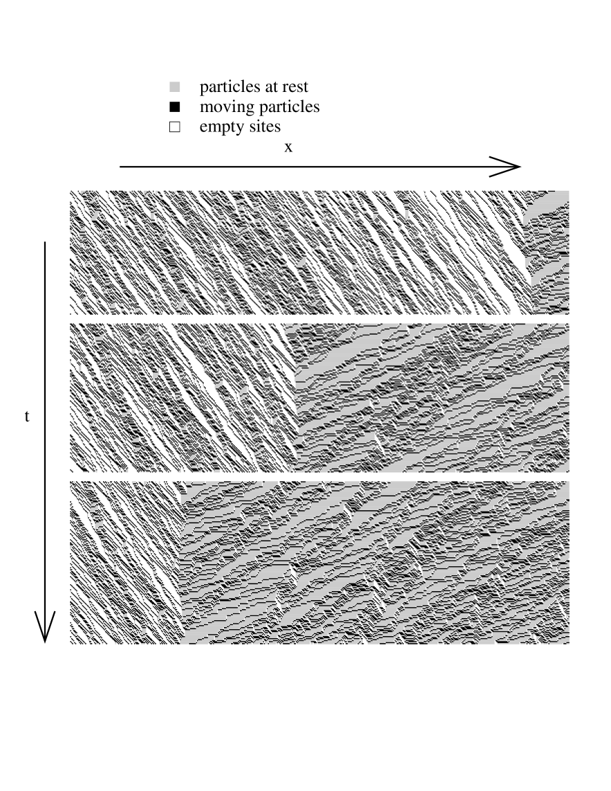
Figure 5: The space-time diagram for $p=0.75,\alpha=\beta=0.3$. The microscopic shock moves freely on the chain.

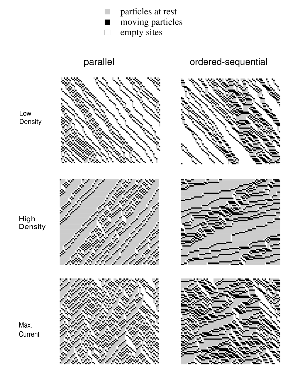
Figure 6: Typical space-time diagrams for the various phases.

Figure 7: Density profiles for parallel update (p=0.75) in the low-density phases AI and AII. The insert compares the exact asymptotic form with a pure exponential decay.

Figure 8: Log-Log plot of the correlation length for different types of updates (OS=ordered-sequential, PARA=parallel, RS=random-sequential). The length scales are obtained from an exponential fit of the density profile, $\alpha$ and $\beta$ are chosen such that $\alpha+\beta=0.6$ holds $(\alpha_{c}=0.3)$.

Figure 9: Density profiles near the first order transition at $\alpha=\beta=0.3$ for the random sequential update using the exact results of [15]. Again $\alpha+\beta=0.6$ holds.

Figure 10: Divergence of the correlation length $\xi_{\alpha}$ near the transition to the maximum current phase ($\beta=0.75$).

Figure 11: Density profile of the pair probabilities $P_{\tau_{i}\tau_{i+1}}$ for the parallel update in the low density phase AII ($\alpha=0.40,\beta=0.75,p=0.75$).

References

- [1] V. Privman (Ed.), Nonequilibrium Statistical Mechanics in One Dimension (Cambridge University Press, 1997)
- [2] B. Schmittmann and R.K.P. Zia, Statistical Mechanics of Driven Diffusive Systems (Academic Press, 1995)
- [3] H. Spohn, Large Scale Dynamics of Interacting Particles (Springer, 1991)
- [4] T.M. Ligett, Interacting Particle Systems (Springer, 1985)
- [5] S. Katz, J.L. Lebowitz and H. Spohn, Nonequilibrium steady states of stochastic lattice gas models of fast ionic conductors, J. Stat. Phys. 34, 497 (1984)
- [6] L. Garrido, J. Lebowitz, C. Maes and H. Spohn, Long-range correlations for conservative dynamics, Phys. Rev. A42, 1954 (1990)
- [7] G.M. Schütz, Experimental realizations of integrable reaction-diffusion processes in biological and chemical systems, cond-mat/9601082
- [8] M. Schreckenberg, A. Schadschneider, K. Nagel and N. Ito, Discrete stochastic models for traffic flow, Phys. Rev. E51 2339 (1995)
- [9] B. Derrida and M.R. Evans, The asymmetric exclusion model: Exact results through a matrix approach, in [1]
- [10] P. Meakin, P. Ramanlal, L. Sander and R.C. Ball, Ballistic deposition on surfaces, Phys. Rev. A34, 5091 (1986)
- [11] M. Kardar, G. Parisi and Y.C. Zhang, Dynamic scaling of growing interfaces, Phys. Rev. Lett. 56, 889 (1986)
- [12] J. Krug, Boundary-induced phase transitions in driven diffusive systems, Phys. Rev. Lett. 67, 1882 (1991)
- [13] B. Derrida, E. Domany and D. Mukamel, An exact solution of a one-dimensional asymmetric exclusion model with open boundaries, J. Stat. Phys. 69, 667 (1992)
- [14] G. Schütz and E. Domany, Phase transitions in an exactly solvable one-dimensional exclusion process, J. Stat. Phys. 72, 277 (1993)
- [15] B. Derrida, M.R. Evans, V. Hakim and V. Pasquier, Exact solution of a 1d asymmetric exclusion model using a matrix formulation, J. Phys. A: Math Gen. 26, 1493 (1993)
-
[16]
A. Klümper, A. Schadschneider and J. Zittartz,
Equivalence and solution of anisotropic spin-1 models and generalized
fermion models in one dimension, J. Phys. A: Math Gen. 24, L955 (1991);
Groundstate properties of a generalized VBS-model, Z. Phys. B87, 281 (1992);
Matrix-product-groundstates for one-dimensional spin-1 quantum antiferromagnets, Europhys. Lett. 24 293 (1993) - [17] R.B. Stinchcombe and G.M. Schütz, Application of operator algebras to stochastic dynamics and the Heisenberg chain, Phys. Rev. Lett. 75 140 (1995)
- [18] K. Mallick, Shocks in the asymmetry exclusion model with an impurity, J. Phys. A: Math Gen. 29, 5375 (1996)
- [19] H. Hinrichsen and S. Sandow, Deterministic exclusion process with a stochastic defect: Matrix product ground states, J. Phys. A: Math Gen. 30, 2745 (1997)
- [20] M.R. Evans, D.P. Foster, C. Godrèche and D. Mukamel, Asymmetric exclusion model with two species: Spontaneous symmetry breaking, J. Stat. Phys. 80, 69 (1995)
- [21] H. Hinrichsen, S. Sandow and I. Peschel, On matrix product ground states for reaction-diffusion models, J. Phys. A: Math Gen. 29, 2643 (1996)
- [22] F.C. Alcaraz, M. Droz, M. Henkel and V. Rittenberg, Reaction-diffusion processes, critical dynamics and quantum chains, Ann. Phys. 230, 250 (1994)
- [23] K. Krebs and S. Sandow, Matrix product eigenstates for one-dimensional stochastic models and quantum spin chains, J. Phys. A: Math Gen. 30, 3165 (1997)
- [24] N. Rajewsky and M. Schreckenberg, Exact results for one dimensional stochastic cellular automata for different types of updates, Physica A245, 139 (1997)
- [25] G. Le Caër, Comparision between simultaneous and sequential updating in cellular automata, Physica A157, 669 (1989)
- [26] H. Hinrichsen, Matrix product ground states for exclusion processes with parallel dynamics, J. Phys. A: Math Gen. 29, 3659 (1996)
- [27] G.M. Schütz, Time-dependent correlation functions in a one-dimensional asymmetric exclusion process, Phys. Rev. E47, 4265 (1993)
- [28] N. Rajewsky, A. Schadschneider and M. Schreckenberg, The asymmetric exclusion model with sequential update, J. Phys. A: Math Gen. 29, L305 (1996)
- [29] A. Honecker and I. Peschel, Matrix-product states for a one-dimensional lattice gas with parallel dynamics, J. Stat. Phys. 88, 319 (1997)
- [30] M. Fannes, B. Nachtergaele and R. Werner, Finitely correlated states on quantum spin chains, Comm. Math. Phys. 144, 443 (1992)
- [31] V. Hakim and J.P. Nadal, Exact results for 2d directed animals on a strip of finite width, J. Phys. A: Math Gen. 16, L213 (1983)
- [32] H. Niggemann and J. Zittartz, Optimum ground states for spin- chains, Z. Phys. B101, 289 (1996)
- [33] F.H.L. Essler and V. Rittenberg, Representations of the quadratic algebra and partially asymmetric diffusion with open boundaries, J. Phys. A: Math Gen. 29, 3375 (1996)
- [34] K. Mallick and S. Sandow, Finite dimensional representations of the quadratic algebra: Applications to the exclusion process, cond-mat/9705152
-
[35]
P.F. Arndt, T. Heinzel and V. Rittenberg, Stochastic
models on a ring and quadratic algebras. The three species diffusion problem,
cond-mat/9703182,
F.C. Alcaraz, S. Dasmahapatra and V. Rittenberg, N-species stochastic models with boundaries and quadratic algebras, cond-mat/9705172 - [36] A. Schadschneider and M. Schreckenberg, Cellular automaton models and traffic flow, J. Phys. A: Math Gen. 26, L679 (1993)
- [37] M.R. Evans, Exact steady states of disordered hopping particle models with parallel and ordered sequential dynamics, J. Phys. A: Math Gen. 30 (1997)
- [38] N. Rajewsky, Exact results for one-dimensional stochastic processes, Dissertation (Universität zu Köln, 1997)
- [39] N. Rajewsky, L. Santen, A. Schadschneider and M. Schreckenberg, The asymmetric exclusion model with time continous and time non-continous update, in “Proceedings of the 1996 Conference on Scientific Computing in Europe”, Eds.: H.J. Ruskin, R. O’Connor, Y. Feng (published by Centre for Teaching Computing, Dublin City University, 1996)
- [40] A. Schadschneider and M. Schreckenberg, Car-oriented mean-field theory for traffic flow models, J. Phys. A: Math Gen. 30, L69 (1997)
- [41] J. Krug and P.A. Ferrari, Phase transitions in driven diffusive systems with random rates, J. Phys. A: Math Gen. 29, L465 (1996)
- [42] D.V. Ktitarev, D. Chowdhury and D.E. Wolf, Stochastic traffic model with random deceleration probabilities: queueing and power-law gap distribution, J. Phys. A: Math Gen. 30, L221 (1997)
- [43] S. Sandow, Partially asymmetric exclusion process with open boundaries, Phys. Rev. E50, 2660 (1994)
- [44] N. Ito, Discrete-time and single-spin-flip dynamics of the Ising chain, Prog. Theor. Phys. 83, 682 (1990)
- [45] B. Eisenblätter, L. Santen, A. Schadschneider and M. Schreckenberg, Jamming transition in a cellular automaton model for traffic flow, Phys. Rev. E , in press (1997) (cond-mat/9706041)
- [46] A. Schadschneider and M. Schreckenberg, Garden of Eden states in traffic models, in preparation
-
[47]
B. Chopard, P.O. Luthi and P.-A. Queloz,
Cellular automata model of car traffic in a two-dimensional street network,
J. Phys. A: Math Gen. 29, 2325 (1996)
B. Chopard, in Proceedings of the Workshop on “Traffic and Granular Flow 1997” (to be published) - [48] J. Esser and M. Schreckenberg, Microscopic simulation of urban traffic based on cellular automata, Int. J. Mod. Phys. C, in press (1997)
- [49] M. Rickert and K. Nagel, Experiences with a simplified microsimulation for the Dallas/Fort Worth area, Int. J. Mod. Phys. C8, 483 (1997)
- [50] K. Nagel and C.L. Barrett, Using microsimulation feedback for trip adaptation for realistic traffic in Dallas, Int. J. Mod. Phys. C8, 505 (1997)
- [51] S. Tadaki, Two-dimensional cellular automaton model of traffic flow with open boundary conditions, Phys. Rev. E54, 2409 (1996)
- [52] N. Rajewsky, R . Raupach and J. Zittartz, in preparation
- [53] A.K. Kolezhuk and H.-J. Mikeska, A new family of models with exact ground states connecting smoothly the S=1/2 dimer and S=1 Haldane phases of 1D spin chains, cond-mat/9701089 (and refs. therein)
- [54] J. Zittartz, in preparation
- [55] R.K.P. Zia and B. Schmittmann, Surprises in simple driven systems: Phase transitions in a three-state model, Int. J. Mod. Phys. C7, 409 (1996)
- [56] T. Sasamoto, S . Mori and M. Wadati, One-dimensional asymmetric exclusion model with open boundaries, J. Phys. Soc. Jpn. 65, 2000 (1996)
Table