Interaction Constants and Dynamic Conductance of a Gated Wire

Abstract

We show that the interaction constant governing the long-range electron-electron interaction in a quantum wire coupled to two reservoirs and capacitively coupled to a gate can be determined by a low frequency measurement. We present a self-consistent, charge and current conserving theory of the full conductance matrix. The collective excitation spectrum consists of plasma modes with a relaxation rate which increases with the interaction strength and is inversely proportional to the length of the wire. The interaction parameter is determined by the first two coefficients of the out-of-phase component of the dynamic conductance measured at the gate.

The comparison of interacting electron theories and experiments often suffers from the fact that the interaction constants are not known. In particular, this is true for interacting quantum wires, where Luttinger models with a wide range of coupling parameters are discussed [1, 2]. Moreover, a single experiment is often not sufficient to determine the coupling constant. Thus, as will be shown, the capacitance (per unit length) of a wire above a back gate is related to the interaction parameter $g$ via

$$c_{\mu}=g^{2}{e^{2}}\nu_{F}.$$ (1)

Since the density of states $\nu_{F}=2/hv_{F}$ (evaluated at constant interaction potential [3]) is generally not known, a capacitance measurement alone cannot determine the interaction constant. Here we propose to investigate the frequency dependence of current induced into the gate. Compared to the measurement of a frequency dependent conductance at a direct contact, the measurement of the gate current can be performed at relatively small frequencies in the kHz range, since the frequency response is not on top of a possibly large dc-conductance. Recently considerable advances have been made in the high precision frequency measurement of the complex ac conductance [4] and the frequency dependent noise [5] of mesoscopic conductors. In this Letter we consider a simple model system – a perfect ballistic wire coupled capacitively to a gate and connected to two electron reservoirs – and calculate the dynamic conductance matrix. While the dc-conductance in this system is quantized and thus provides no information on the interaction, the dynamic conductance is a sensitive function of the interaction strength.

A conceptually important point which needs to be addressed in solving this problem is the coupling of an interacting wire to electron reservoirs. Previous works [6] have proposed a purely one-dimensional model in which the interaction changes from a value $g<1$ (characteristic of interactions) to a value $g=1$ (characterizing a system without interactions) at the transition from the ballistic wire to the electron reservoir. Another more recent proposal [7] consists of a radiative boundary condition in which the electron density is proportional to the applied voltage. In this work we use a concept of reservoirs based on the electrochemical nature of electric transport[3]. The electron density in the wire is the sum of two terms: a chemical density, which follows the chemical potential of the reservoir from which the carriers are injected into the wire, and an induced density, which results from the (long range) Coulomb screening of the injected charge. Indeed, from a screening point of view electrons in a reservoir are not free: an increase of the electrochemical potential is followed by an equal increase in the electrostatic potential. That corresponds to strong interaction (very effective three-dimensional screening) in a reservoir rather than to a non-interacting one-dimensional (1D) model with $g=1$. Similarly, the radiative boundary condition employed in Ref. [7] is not correct: in a reservoir an increase of a voltage leaves the local density invariant. These divergent views arise from the fact that interactions play a role on very different length scales [8]. Different interaction parameters must be used to describe long range and short range effects [9]. Conceptually, Ref. [10], which describes the reservoirs by the charges, conjugate to the chemical reservoir potentials, is closest to our approach.

Ballistic single mode wires [1, 2] coupled to reservoirs are the simplest model system in which these questions are significant. The dynamic response of 1D interacting systems has been investigated previously in the framework of the Luttinger model by several authors [11, 12, 13]. The results obtained in these works are, however, not charge and current conserving (gauge invariant) [14]. Below we present results for the ac conductance of an interacting quantum wire, connected to two reservoirs and capacitively coupled to a gate. On a length scale large compared to the distance between the wire and the gate the interactions can be treated as short ranged. Our discussion explicitly includes the effect of the gate. Of interest is the displacement current which flows from the wire to the gate and which we propose to measure to determine the interaction constant.

Consider the system depicted in Fig. 1, consisting of a 1D quantum wire of length $L$, connected to two reservoirs at $x=0$ and $x=L$. The potential in the left (1) reservoir is modulated in time, $V_{1}(t)=V_{1,\omega}e^{-i\omega t}$, whereas the potential in the right (2) reservoir is kept constant. We treat the interactions in random phase approximation (RPA). For electron densities which are not too small ($e^{2}/hv_{F}<1$, where $v_{F}$ is the Fermi velocity), RPA is essentially exact. We note also that even within the strict limits of RPA validity the interaction constant $g$ may still be made small by appropriate choice of capacitance between the wire and the gate, see Eq. (6) below.

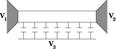
FIG. 1.: The 1D wire, connected to two reservoirs and coupled capacitively to a gate.

Self-consistent potential. In the absence of interactions, a potential modulation in the left reservoir injects a bare charge density $\rho_{0,\omega}(x)$ into the wire,

$$\rho_{0,\omega}(x)=\frac{\nu_{F}V_{1,\omega}}{2}e^{iq_{F}x},$$ (2)

where $\nu_{F}=2/hv_{F}$ is the density of states at the Fermi level ($v_{F}$ is the Fermi velocity), and $q_{F}=\omega/v_{F}$.

In the presence of an external potential $\phi_{\omega}(x)/e$, the true charge density is

$$\rho_{\omega}(x)=\rho_{\omega,0}(x)-\int\limits_{0}^{L}dx^{\prime}\Pi_{\omega}(x,x^{\prime})\phi_{\omega}(x^{\prime}),$$ (3)

where the polarization kernel is given by (see e.g. [15])

$$\Pi_{\omega}(x,x^{\prime})=\nu_{F}\delta(x-x^{\prime})+\frac{iq_{F}\nu_{F}}{2}e^{iq_{F}|x-x^{\prime}|}.$$ (4)

Eq. (3) gives the charge density as a sum of two contributions: a chemical one, proportional to the potential $V_{1,\omega}$ of the reservoir, and an induced component, proportional to the electrostatic potential.

We now take electron-electron interactions into account by determining the actual potential $\phi_{\omega}(x)$ in the wire self-consistently, i.e., by relating the total charge $\rho_{\omega}$ on the left hand side of Eq. (3) to the potential $\phi_{\omega}$. In order to do this, we need to specify the electron-electron interaction. In the case of bare Coulomb interactions, the required relation is the Poisson equation $\Delta\phi_{\omega}=-4\pi e^{2}\rho_{\omega}$. For short-ranged interactions this relation is different and is found as follows: Generally, the interaction potential $V(\mathchoice{{\hbox{\boldmath$\displaystyle r$}}}{{\hbox{\boldmath$\textstyle r$}}}{{\hbox{\boldmath$\scriptstyle r$}}}{{\hbox{\boldmath$\scriptscriptstyle r$}}},\mathchoice{{\hbox{\boldmath$\displaystyle r^{\prime}$}}}{{\hbox{\boldmath$\textstyle r^{\prime}$}}}{{\hbox{\boldmath$\scriptstyle r^{\prime}$}}}{{\hbox{\boldmath$\scriptscriptstyle r^{\prime}$}}})$ is the Green’s function for the operator equation $\hat{K}V(\mathchoice{{\hbox{\boldmath$\displaystyle r$}}}{{\hbox{\boldmath$\textstyle r$}}}{{\hbox{\boldmath$\scriptstyle r$}}}{{\hbox{\boldmath$\scriptscriptstyle r$}}},\mathchoice{{\hbox{\boldmath$\displaystyle r^{\prime}$}}}{{\hbox{\boldmath$\textstyle r^{\prime}$}}}{{\hbox{\boldmath$\scriptstyle r^{\prime}$}}}{{\hbox{\boldmath$\scriptscriptstyle r^{\prime}$}}})=4\pi e^{2}\delta(\mathchoice{{\hbox{\boldmath$\displaystyle r$}}}{{\hbox{\boldmath$\textstyle r$}}}{{\hbox{\boldmath$\scriptstyle r$}}}{{\hbox{\boldmath$\scriptscriptstyle r$}}}-\mathchoice{{\hbox{\boldmath$\displaystyle r^{\prime}$}}}{{\hbox{\boldmath$\textstyle r^{\prime}$}}}{{\hbox{\boldmath$\scriptstyle r^{\prime}$}}}{{\hbox{\boldmath$\scriptscriptstyle r^{\prime}$}}})$. The same operator $\hat{K}$ also connects charge $\rho$ and potential $\phi$ via $\hat{K}\phi(\mathchoice{{\hbox{\boldmath$\displaystyle r$}}}{{\hbox{\boldmath$\textstyle r$}}}{{\hbox{\boldmath$\scriptstyle r$}}}{{\hbox{\boldmath$\scriptscriptstyle r$}}})=4\pi e^{2}\rho(\mathchoice{{\hbox{\boldmath$\displaystyle r$}}}{{\hbox{\boldmath$\textstyle r$}}}{{\hbox{\boldmath$\scriptstyle r$}}}{{\hbox{\boldmath$\scriptscriptstyle r$}}}).$ For bare Coulomb interactions, $\hat{K}$ is the Laplace operator $\Delta$, and the Poisson equation follows. Here we consider short range interactions characterized by the interaction strength $V_{0}$, $V(x-x^{\prime})=V_{0}\delta(x-x^{\prime})$. In this case the operator $\hat{K}$ is just a multiplication with a constant factor $4\pi e^{2}/V_{0}$. Thus, the potential and charge are connected via

$$\phi_{\omega}(x)=V_{0}\rho_{\omega}(x),$$ (5)

instead of the Poisson equation. At this point it therefore is quite natural to introduce the capacitance of the wire per unit length, $c=e^{2}/V_{0}$. Physically, this corresponds to a single mode quantum wire, formed by depletion induced by a back-gate with a capacitance $c$ per unit length, parallel to the wire (see Fig. 1). The well-known interaction parameter $g$ of the LL is then related to the capacitance $c$ [16] via

$$g^{2}=\frac{1}{1+e^{2}\nu_{F}/c}.$$ (6)

In particular, the case of the locally charge neutral wire[15], corresponds to $c=0$ or infinitely strong point-like interactions ($g=0$). Indeed, the single-channel results of Ref. [15] are obtained as the $g\to 0$ limit of the formulas derived below.

Now we generalize our approach to the case when the back-gate is modulated by a potential $V_{3}(t)=V_{3,\omega}e^{-i\omega t}$ as well. Then the total density of the wire contains in addition to the density injected from reservoir $1$ an induced density due to the modulation of the gate. The self-consistent potential distribution $\phi_{\omega}(x)$ along the wire must now be found from the equation

$$\frac{c}{e^{2}\nu_{F}}\left(\phi_{\omega}(x)-V_{3,\omega}\right)=\frac{V_{1,\omega}}{2}e^{iq_{F}x}-\phi_{\omega}(x)-\frac{iq_{F}}{2}\int\limits_{0}^{L}dx^{\prime}e^{iq_{F}|x-x^{\prime}|}\phi_{\omega}(x^{\prime}),$$ (7)

which is obtained by substituting $\phi_{\omega}(x)-V_{3,\omega}$ in the lhs of Eq. (5) and using Eq. (3). The solution to Eq. (7) is

$$\phi_{\omega}(x)=V_{3,\omega}+A^{+}_{\omega}e^{iqx}+A^{-}_{\omega}e^{-iqx},$$ (8)

where $q=gq_{F}$, and

$$A^{\pm}_{\omega} = \pm\frac{(1\pm g)(1-g^{2})e^{\mp iqL}}{(1+g)^{2}e^{-iqL}-(1-g)^{2}e^{iqL}}$$ (9)

$$\times \left[V_{1,\omega}-V_{3,\omega}\left(1-\frac{1\mp g}{1\pm g}e^{\pm iqL}\right)\right].$$ (10)

Conductance matrix. With the true potential we are now in a position to find the full conductance matrix for the capacitively coupled wire. The conductance matrix ${\cal G}_{\alpha\beta}(\omega)$ relates the current $I_{\alpha,\omega}$ at contact $\alpha$ to the voltage $V_{\beta,\omega}$ applied at contact $\beta$ ($\alpha,\beta=1,2,3$): $I_{\alpha,\omega}={\cal G}_{\alpha\beta}(\omega)V_{\beta,\omega}$. With the definitions

$$G_{\omega}=2g\frac{e^{2}}{h}\frac{(1+g)e^{-iqL}+(1-g)e^{iqL}}{(1+g)^{2}e^{-iqL}-(1-g)^{2}e^{iqL}}$$ (11)

and

$$\bar{G}_{\omega}=-\frac{e^{2}}{h}\frac{4g}{(1+g)^{2}e^{-iqL}-(1-g)^{2}e^{iqL}},$$ (12)

the conductance matrix takes a form

$${\cal G}(\omega)=\left(\begin{array}[]{ccc}G_{\omega}&\bar{G}_{\omega}&-G_{\omega}-\bar{G}_{\omega}\\ \bar{G}_{\omega}&G_{\omega}&-G_{\omega}-\bar{G}_{\omega}\\ -G_{\omega}-\bar{G}_{\omega}&-G_{\omega}-\bar{G}_{\omega}&2G_{\omega}+2\bar{G}_{\omega}\end{array}\right).$$ (13)

The matrix ${\cal G}$ has the following properties [3]: First, it is symmetric, which reflects the fact that the geometry considered here is symmetric under the exchange of the left and right reservoir, and no magnetic field is present. Then, $\sum_{\alpha}{\cal G}_{\alpha\beta}=0$, which re-states current conservation. Finally, the property $\sum_{\beta}{\cal G}_{\alpha\beta}=0$ manifests the fact that a simultaneous shift of all potentials $V_{\beta}$ by the same amount does not produce any current (gauge invariance). Furthermore, dissipation of power requires that the matrix ${\rm Re}\ \cal{G}$ is positive definite.

In the static limit $\omega=0$ one reproduces the known result [6]: $G=-\bar{G}=e^{2}/h$, with no current flowing through the gate. Another limiting case is $g=0$ [15], where one finds $G=-\bar{G}=(e^{2}/h)(1-iq_{F}L/2)^{-1}$. Generally, all the components of the conductance matrix are oscillating functions of frequency (for $g\neq 0$) with the period $2\pi v_{F}(gL)^{-1}$. In particular, the real part of the conductance reaches zero with a period $2\pi v_{F}(gL)^{-1}$. It has been suggested that measurement of this period should be used to determine the interaction constant [12, 13]. However, this period is a consequence of the linearization of the spectrum near the Fermi energy and not really a signature of an interacting system. Furthermore, this frequency is already in the absence of interactions of the order of an electron transit frequency and therefore rather high. A much better strategy consists in analyzing one of the purely capacitive conductances between the wire and the gate. In particular, we consider ${\cal G}_{33}(\omega)=2(G_{\omega}+\bar{G}_{\omega})$, which we call the gate conductance. The real and imaginary parts of the frequency dependence of the gate conductance ${\cal G}_{33}(\omega)$ are displayed in Fig. 2. The real part shows peaks around $\omega=(\pi v_{F}/gL)(2n+1)$, $n\in\cal{Z}$. The height of each peak is equal to four times the conductance quantum $e^{2}/h$ (and thus independent of $g$), while the width decreases with decreasing $g$. In contrast, the imaginary part of ${\cal G}_{33}(\omega)$ changes sign at these points, and exhibits extrema (sharp ones for small $g$) at the points

$$\Omega_{n}=\frac{v_{F}}{gL}\left[\pi(2n+1)\pm\arccos\frac{1-g^{2}}{1+g^{2}}\right].$$

The height of each peak is $2e^{2}/h$.

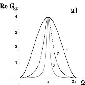
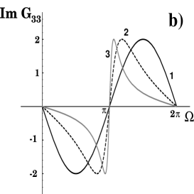
FIG. 2.: One period of the frequency dependence of the real (a) and imaginary (b) parts of the gate conductance ${\cal G}_{33}(\omega)$ (in units $e^{2}/h$). The parameter $g$ is equal to 1 (curve 1), 0.3 (2), and 0.1 (3); the argument is $\Omega=\omega Lg/v_{F}$.

All elements of the conductance matrix ${\cal G}_{\alpha\beta}$ are characterized by the common denominator $(1+g)^{2}e^{-iqL}-(1-g)^{2}e^{iqL}$, which has zeros at frequencies

$$\omega_{n}=\frac{v_{F}}{gL}\left[n\pi-i\ln\frac{1+g}{1-g}\right].$$ (14)

Eq. (14) defines the (collective) excitation spectrum of the quantum wire. For $g=0$ (local charge neutrality) only the $n=0$ mode survives, and all other frequencies are pushed up to infinity. This mode is purely imaginary, and does not correspond to any type of quasiparticles [15]. On the other hand, for $g=1$ (non-interacting system) all modes are infinitely damped: Thus, charge relaxation can only be caused by electron-electron interactions. We mention that the same modes are obtained in Ref. [12]; the modes with even $n$ are also obtained in Ref. [13]. Any treatment, whether self-consistent or not, which at some stage invokes the effective interaction, will exhibit this frequency spectrum.

We have now characterized the dynamic conductance and its properties over a wide frequency range. But it is the low frequency regime that is experimentally most easily accessed. A low frequency measurement works only if we consider the gate current since at small frequencies the ac component of the conductance ${\cal G}_{11}$ represents only a small deviation from the quantized dc-conductance and is hard to identify[17]. The gate conductance has the following low frequency expansion

$${\cal G}_{33}=-iC_{\mu}\omega+R_{q}C^{2}_{\mu}\omega^{2}-i\frac{1-3g^{2}}{3g^{2}}R_{q}^{2}C^{3}_{\mu}\omega^{3}+\dots$$

Here $C_{\mu}=c_{\mu}L$ is the total electrochemical capacitance of the wire vis-a-vis the gate, $c_{\mu}$ is given by Eq. (1). The second order term is determined by the charge relaxation resistance[18] $R_{q}=h/4e^{2}$ which is the parallel resistance of two Sharvin-Imry contact resistances of half a resistance quantum per contact. It is independent of the interaction constant. The third order term is proportional to the third power of the electrochemical capacitance $C_{\mu}$, but most importantly it is proportional to a factor $1/3g^{2}-1$, which is a sensitive function of the interaction strength. Thus, a measurement which determines the out-of-phase (non-dissipative) part of the gate conductance up to the the third order in frequency is sufficient to determine the interaction parameter $g$.

Conclusions. We have investigated the ac response of a quantum wire with short-range interactions. We formulated a self-consistent, charge and current conserving approach using RPA. For a wire with a density which is not too small, RPA captures the essential physics. The boundary condition which couples the density of the wire to the electron reservoirs is of eletrochemical nature. Due to the coupling with the reservoir all the collective modes of the system acquire a damping constant. In the present paper the one-channel case is considered only. The case of two channels with the same velocity $v_{F}$ (corresponding to one spin-degenerate channel) can be obtained from the above results simply by replacing the density of states of the one-channel problem $\nu$ by that appropriate for the spin-degenerate channel $2\nu$: Spin–charge separation can not be probed by the ac response.

We find that the measurement of the low-frequency, non-dissipative component of the gate conductance including only its first two leading coefficients is sufficient to determine the interaction strength. Such measurements are very desirable and will provide a strong stimulation for further research on the role of electron-electron interactions.

We acknowledge the financial support of the Swiss National Science Foundation and of the European Community (Contract ERB-CHBI-CT941764).

REFERENCES

- [1] F. D. M. Haldane, J. Phys. C 14, 2585 (1981); C. L. Kane and M. P. A. Fisher, Phys. Rev. B 46, 15233 (1992).
- [2] S. Tarucha, T. Honda, and T. Saku, Solid State Commun. 94, 413 (1995); A. Yacoby et al., Phys. Rev. Lett. 77, 4612 (1996).
- [3] M. Büttiker, J. Phys. Condensed Matter 5, 9361 (1993).
- [4] J. B. Pieper and J. C. Price, Phys. Rev. Lett. 72, 3586 (1994).
- [5] R. J. Schoelkopf et al., Phys. Rev. Lett. 78, 3370 (1997).
- [6] D. L. Maslov and M. Stone, Phys. Rev. B 52, R5539 (1995); V. V. Ponomarenko, ibid 52, R8666 (1995); I. Safi and H. J. Schulz, ibid 52, R17040 (1995).
- [7] R. Egger and H. Grabert, Phys. Rev. Lett. 77, 538 (1996).
- [8] D. Pines and P. Nozières, The Theory of Quantum Liquids (W. A. Benjamin, N. Y., 1966).
- [9] Models for fractional edge states fix according to the relevant ground state, see X. G. Wen, Phys. Rev. B 41, 12838 (1990). The interaction due to long range Coulomb forces has to be included via an additional interaction parameter.
- [10] A. Yu. Alekseev, V. V. Cheianov, and J. Fröhlich, cond-mat/9706061 (unpublished).
- [11] G. Cuniberti, M. Sassetti, and B. Kramer, J. Phys.: Condens. Matter 8, L21 (1996); cond-mat/9710053 (unpublished).
- [12] V. V. Ponomarenko, Phys. Rev. B 54, 10328 (1995).
- [13] V. A. Sablikov and B. S. Shchamkhalova, Pis’ma Zh. Éksp. Teor. Fiz. 66, 40 (1997) [JETP Lett. 66, 41 (1997)].
- [14] The necessity of a self-consistent calculation of the electric field was stressed for the dc problem by A. Kawabata, J. Phys. Soc. Jap. 65, 30 (1996); cond-mat/9701171 (unpublished); Y. Oreg and A. M. Finkel’stein, Phys. Rev. B 54, R14265 (1996).
- [15] Ya. M. Blanter and M. Büttiker, cond-mat/9706070 (unpublished).
- [16] The equivalence between the LL model with short-range interaction and a gated wire was noted by L. I. Glazman, I. M. Ruzin, and B. I. Shklovskii, Phys. Rev. B 45, 8454 (1992); K. A. Matveev and L. I. Glazman, Physica B 189, 266 (1993); see also R. Egger and H. Grabert, cond-mat/9709047 (unpublished).
- [17] W. Chen, T. P. Smith III, M. Büttiker, and M. Shayegan, Phys. Rev. Lett. 73, 146 (1994).
- [18] M. Büttiker, H. Thomas, and A. Prêtre, Phys. Lett. A 180, 364 (1993).