Numerical analysis of the bond-random antiferromagnetic $S=1$ Heisenberg chain

Abstract

Ground state of the bond-random antiferromagnetic $S=1$ Heisenberg chain with the biquadratic interaction $-\beta\sum_{i}({\bf S}_{i}\cdot{\bf S}_{i+1})^{2}$ is investigated by means of the exact-diagonalization method and the finite-size-scaling analysis. It is shown that the Haldane phase $\beta\approx 0$ persists against the randomness; namely, no randomness-driven phase transition is observed until at a point of extremely-broad-bond distribution. We found that in the Haldane phase, the magnetic correlation length is kept hardly changed. These results are contrastive to those of an analytic theory which predicts a second-order phase transition between the Haldane and the random-singlet phases at a certain critical randomness.

1 Introduction

The ground-state phase transition of the disordered quantum system has attracted much attention recently [1]. Because the transition is driven solely by the quantum fluctuation, the transition lies in different universality from the finite-temperature transitions. The randomness contributes significantly to the anisotropy of the real-space and the imaginary-time directions. Thereby, the randomness would also promote new types of phase transition.

For this purpose, the ground state of the random quantum spin system has been studied considerably, see the article [1, 2] for a review. In one dimension, in particular, a real-space-decimation procedure [3, 4] yields various definite predictions [5, 6, 7]. For the Heisenberg model in the presence of the bond randomness [6, 8, 9], for example, the theory tells that infinitesimal randomness drives the ground state to the random-singlet phase, where the averaged ground-state correlation decays obeying the power law,

$$\left[\langle S^{\alpha}_{0}S^{\alpha}_{r}\rangle\right]_{\rm av}\sim 1/r^{2}\ .$$ (1)

Note that the correlation decays faster than that of the pure chain $\sim 1/r$. Numerical simulations followed [10, 11, 12] so as to confirm the analytic predictions. It would be noteworthy that the $S=1/2$ spin system is viewed as a hard-core boson system [13]. The random spin system is, thus, equivalent to the strongly repulsive boson system embedded in a certain randomness, which is of the current interest [14].

In these studies, the magnitude of the constituent spin is set to be one half. In one dimension, however, there exist some other sorts of magnets such as the integer-spin Heisenberg chain and the $S=1/2$ Heisenberg ladder model. The ground states of these magnets are different from the ground state of the $S=1/2$ Heisenberg chain [15, 16]: In the former case, a finite magnetic excitation gap opens above the ground state, and the magnetic correlation decays exponentially in the ground state. In the present paper, we investigate the bond-random antiferromagnetic $S=1$ spin chain. The Hamiltonian is given by

$${\cal H}=\sum_{i=1}^{L}J_{i}\left\{{\bf S}_{i}\cdot{\bf S}_{i+1}-\beta({\bf S}_{i}\cdot{\bf S}_{i+1})^{2}\right\}.$$ (2)

The operators ${\bf S}_{i}=(S^{x}_{i},S^{y}_{i},S^{z}_{i})$ denote the $S=1$ spin operators acting on the site $i$, and satisfy the periodic boundary condition, ${\bf S}_{L+1}={\bf S}_{1}$. We used the following bond distribution, see Fig. 1,

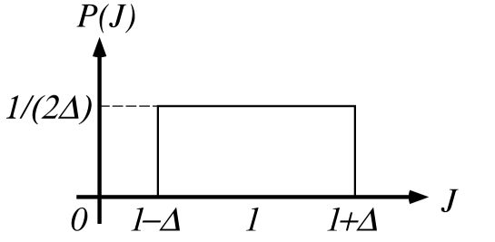
Figure 1: The probability distribution of the random bond $J$. The randomness ranges as $0\leq\Delta\leq 1$. At $\Delta=1$, the distribution becomes extremely broad; namely, infinitesimally weak bond appears.

$$P_{\Delta}(J)=\frac{1}{2\Delta}\left(\Theta(J-1+\Delta)-\Theta(J-1-\Delta)\right)\ .$$ (3)

(The function $\Theta(x)$ denotes the step function.) Note that only the antiferromagnetic bond appears.

Because of the presence of the excitation gap, the system (2) lies beyond the scope of the previous studies of the $S=1/2$ magnets explained above. It is quite suggestive that the real-space decimation theory becomes inapplicable for the cases other than $S=1/2$. In order to adapt the decimation procedure even for the case $S=1$, several authors proposed schemes to map the random $S=1$ chain to an effective $S=1/2$ model [17, 18]. Their theory and the consequences are reviewed afterwards.

The effect of the non-magnetic impurity doping upon the spin-gap ground state has been considered rather throughly [19, 20, 21]: The non-magnetic impurity causes notable influences for the Heisenberg ladder. Infinitesimal doping distracts the spin gap, and gives rise to a magnetically (quasi-)ordered ground state with gapless excitation. The effect of the bond randomness, which is of the present interest, would be more subtle, and remained unsolved.

For the pure system $\{J_{i}=1\}$, the ground-state phase diagram of the Hamiltonian (2) is known, see the paper [27] for details. We explain the region $\beta\sim 0$ relevant to the present study. In the region $-1<\beta<1$, the system is in the Haldane phase, which is mentioned above; namely, a finite excitation gap opens, and the magnetic correlation decays exponentially in the ground state. At the critical point $\beta=1$, the Hamiltonian is integrable. It is predicted in a field-theoretical manner [23] that the criticality is of the central charge $c=3/2$, and the biquadratic interaction generates the excitation gap in the form,

$$\Delta E\propto|\beta-1|^{\nu}\ ,$$ (4)

where $\nu=1$. Numerical simulations have tried to confirm the above scenario [24, 25, 26, 27]. A strong finite-size corrections, however, arise so as to prevent definite conclusions. Typical simulation claims that a transition locates at $\beta\approx 0.5$, and gapless phase extends over $0.5<\beta$ [25, 26]. The inconsistency might be originated in the long correlation length $\xi$ in the Barber-Batchelor phase $1<\beta$; $\xi\approx 21$ at $\beta\to\infty$ [28]. The length apparently exceeds the limit tractable by means of the exact-diagonalization method.

The paper is organized as follows. In the next section, we explain the previous analytic theory employing the real-space-decimation method [17, 18]. The theory predicts that a phase transition separates the Haldane and the random-singlet phases at a certain critical randomness. In the section 3, we present our result by means of the exact diagonalization method. We show that the finite-size scaling assuming the theoretical prediction fails; namely, the present numerical estimate of the transition point and the critical exponent contradicts the prediction. The Haldane phase persists against the randomness until the extremely-broad-bond distribution $\Delta=1$. The results of the correlation length and the spin stiffness confirm the present conclusion. In the last section, we summarize our results, and discuss a possible scenario interpreting our numerical results.

2 Review of the predictions with the real-space decimation analysis

In this section, we review the predictions of the analytic theory [17, 18]. Some are contrastive to our numerical results shown later. As was introduced in the section 1, the real-space-decimation method describes the one-dimensional random magnets quite successfully. The method, however, fails in the cases other than $S=1/2$. Hyman and Yang thus proposed the mapping with which the $S=1$ random chain (2) is transformed to an effective random $S=1/2$ chain. The resultant $S=1/2$ chain constitutes the alternating two types of random bonds, $\{J_{2i}\}$ and $\{J_{2i-1}\}$. The even bonds are either ferromagnetic or antiferromagnetic, whereas the odd bonds are always antiferromagnetic.

We sketch how the effective $S=1/2$ random chain is derived. Suppose a sector within the $S=1$ chain in which sector the deviation of the randomness is incidentally small. They assumed that such sector could be replaced with that without any randomness. As a consequence, the random $S=1$ chain consists of finite uniform $S=1$ sectors coupling antiferromagnetically. On the other hand, it was reported that at an end of the uniform $S=1$ open chain, the $S=1/2$ magnetization appears spontaneously with a certain localization length [29]. Both the end magnetizations couple antiferromagnetically (ferromagnetically), if the length of the open chain is even (odd). Thereby, the finite uniform $S=1$ sector is replaced with the two $S=1/2$ spins coupling either antiferromagnetically or ferromagnetically.

The real-space decimation procedure is employed afterwards. They found a fixed point at a critical randomness $\Delta_{\rm c}$, which separates the Haldane phase and the random-singlet phase [18]. (Refer to the section 1 for these phases.) Furthermore, the theory concludes that the correlation length diverges as

$$\xi\sim 1/|\Delta-\Delta_{\rm c}|^{\nu}$$ (5)

with $\nu\approx 2.3$.

The decimation procedure was simulated numerically as well [30]. The simulation shows that an intermediate phase appears between the Haldane and the random-singlet phases.

3 Numerical results

In this section, we investigate the Hamiltonian (2) by means of the exact-diagonalization method. The exact-diagonalization method has been utilized successfully in the course of the studies of the $S=1/2$ random spin systems [10, 11, 31].

3.1 Suppression of the string correlation by the randomness

In Fig. 2, we plotted the string correlation [32, 33] ${\cal O}^{z}_{\rm string}(L/2)$ against the randomness $\Delta$ at the Heisenberg point $\beta=0$.

Figure 2: The string correlation ${\cal O}_{\rm string}^{z}(L/2)$ (6) is plotted for various randomness $\Delta$ at the Heisenberg point $\beta=0$. The string correlation which characterizes the Haldane phase becomes suppressed as the randomness is strengthened.

The string correlation is defined as

$${\cal O}^{z}_{\rm string}(j-i)=\left[\langle S^{z}_{i}{\rm e}^{{\rm i}\pi\sum_{k=i}^{j-1}S^{z}_{k}}S^{z}_{j}\rangle\right]_{\rm av}\ .$$ (6)

The random average $[\ ]_{\rm av}$ is taken over ninety samples throughout the present study. The string correlation was invented in order to detect characteristics of the Haldane state. The long-range limit was estimated numerically, ${\cal O}^{\alpha}_{\rm string}(r\to\infty)\to 0.38$, at $\beta=0$ [34]. (It is noteworthy that the usual correlations, such as the Néel correlation, are short-range.) In Fig. 2, we see that the string order dominates in the weak-random region, while it becomes suppressed as the randomness is strengthened.

In order to observe whether the string correlation is long-range or not, we evaluate the Binder parameter [35] for the string correlation,

$$U(L)=1-\frac{[\langle O^{4}\rangle]_{\rm av}}{3[\langle O^{2}\rangle]_{\rm av}},$$ (7)

where $O=\sum_{i=1}^{L}{\rm e}^{{\rm i}\pi\sum_{k=1}^{i-1}S^{z}_{k}}S^{z}_{i}$. The Binder parameter is enhanced (suppressed) with increasing the system size, if the corresponding order is long-range (short-range). It is plotted in Fig. 3, where the parameter varies in the same range as that in Fig. 2.

Figure 3: The Binder parameter $U(L)$ (7) is plotted for the same parameter range as that shown in Fig. 2. The plot shows that the string order develops over the whole region, and at the extreme randomness $\Delta=1$, it is disturbed.

We see that the string order develops in the whole range of the randomness. The result contradicts the picture [18] reviewed in the previous section.

As the biquadratic term is turned on ($\beta>0$), the Haldane phase becomes suppressed. (Note the phase diagram for the pure case reviewed in the section 1.) In Fig. 4, where we plotted the Binder parameter at $\beta=0.2$.

Figure 4: The Binder parameter $U(L)$ is plotted for various randomness $\Delta$ at $\beta=0.2$. We see an intersection point $\Delta\sim 0.6$ which suggests a transition point.

It is implied that there exists a transition point $\beta\approx 0.6$; in one side $\beta<0.6$ the string order develops, while in the other side $0.6<\beta$ it is disturbed. Some might wonder that the result of $\beta=0.2$ in Fig. 4 is inconsistent with the result of $\beta=0$ in Fig. 3, and the former supports the picture of the previous theory [18]. In the following, however, we show an evidence that the transition point (intersection point) is extrapolated to $\Delta\approx 1$ in the thermodynamic limit $L\to\infty$.

3.2 Analysis of the transition point

According to the theory [18] reviewed in the section 2, the transition should be the second order. Namely, the Binder parameter (7) obeys the finite-size scaling hypothesis,

$$U(L)=L^{x}\tilde{U}\left((\Delta-\Delta_{\rm c})L^{1/\nu}\right)\ .$$ (8)

The scaling dimension $x$ is zero, because the Binder parameter is dimensionless. Therefore, the data $(\Delta-\Delta_{\rm c})L^{1/\nu})$-$U(L)$, the so-called scaling data, must align along a curve which is independent on the system size $L$. We determine the scaling parameters $\Delta_{\rm c}$ and $\nu$ in eq. (8), so that the data converge to such an universal curve; see the appendix for details.

In Fig. 5, we show the scaling plots for $\beta=0.2$.

Figure 5: Scaling plots for $\beta=0.2$. In order to observe the systematic corrections to the finite size scaling, we managed to analyse different three sets of the system sizes; (a) $L=6,8,10$, (b) $L=8,10,12$ and (c) $L=10,12,14$, respectively.

In order to see the systematic corrections to the finite size scaling, the scaling analyses are managed for different three sets of the system sizes; (a) $L=6,8,10$, (b) $L=8,10,12$ and (c) $L=10,12,14$, respectively. We define the approximative transition point $\Delta(l)$ and the exponent $\nu(l)$, which are determined by the scaling plot $L=l-2,l$ and $l+2$. We found that the scaling parameters result in the following,

$$\Delta_{\rm c}(8)=0.67,\ \Delta_{\rm c}(10)=0.70,\ \Delta_{\rm c}(12)=0.87,$$

$$\nu(8)=0.92,\ \nu(10)=0.76,\ \nu(12)=0.84.$$ (9)

The transition point converges to $\Delta\sim 1$ for large system sizes, and the exponent approaches $\nu\sim 0.9$. It is suggested that the transition point is identical with that at the Heisenberg point $\beta=0$, see Fig. 3.

We show the scaling plots for $\beta=0.3$ as well, see Fig. 6.

Figure 6: Scaling plots for $\beta=0.3$. The analysis is the same as that shown in Figs. 5.

The plots yield the following estimates:

$$\Delta_{\rm c}(8)=0.33,\ \Delta_{\rm c}(10)=0.47,\ \Delta_{\rm c}(12)=0.56,$$

$$\nu(8)=0.65,\ \nu(10)=0.94,\ \nu(12)=0.34.$$ (10)

We observe that the transition point approaches $\Delta\to 1$, while the exponent rather scatters. The scaling analyses beyond $\beta\sim 0.3$ are suffered by strong finite-size corrections which also exist for the uniform system (refer to the section 1). In consequence of the previous and the present subsections, we observe that a phase transition might occur at $\Delta=1$. The universality class is rather ambiguous. It is suggested, at least, that the previous prediction $\nu\approx 2.3$ [18] is not accordant with our numerical analysis.

In the next subsection, we show an evidence that the transition is the first order. Even for such case, the above finite-size-scaling analysis is still meaningful in the sense that it yields the estimate of the intersection point of the Binder parameters. The intersection point is expected to converge to the transition point even for the first-order transition. The exponent, on the contrary, is not universal, and possibly would not be well-defined for very large system sizes.

3.3 Correlation length and the spin-stiffness constant

In order to confirm that a first-order transition takes place at $\Delta=1$, we show the result of the correlation length. We found that the correlation length is remained unchanged over the whole region $0<\Delta<1$; namely, the correlation length does not diverge as in eq. (5).

In Fig. 7, the averaged Néel correlation is plotted for various randomness at the Heisenberg point $\beta=0$.

Figure 7: Logarithm of the Néel correlation ${\cal O}^{z}_{\rm Neel}(L/2)$ is plotted against the system size $L$ for various randomness at the Heisenberg point $\beta=0$. The decay rate ($\sim{\rm e}^{-r/6.2}$) at $\Delta=0$ [36] is shown by the dashed line. The plot shows that the correlation decays exponentially in fact, and the correlation length is not changed very much with increasing the randomness.

The averaged Néel correlation is given by

$${\cal O}^{z}_{\rm Neel}(j-i)=\left[\langle(-1)^{j-i}S^{z}_{i}S^{z}_{j}\rangle\right]_{\rm av}.$$ (11)

The decay rate $\sim{\rm e}^{-(j-i)/6.2}$ estimated previously [36] at $\Delta=0$ is shown as well. The magnetic correlation length is hardly changed with the randomness. Moreover, we observe that the correlation itself is not changed very much. The result indicates that the Haldane phase with finite correlation length $\xi\sim 6.2$ continues up to the extreme point $\Delta=1$.

In Fig. 8, the spin stiffness constant is plotted.

Figure 8: Logarithm of the spin-stiffness constant $\rho_{\rm s}(L)$ is plotted against (a) $L$ and (b) $\log L$, respectively, for various randomness at $\beta=0$.

The stiffness constant [37] is defined by

$$\rho_{\rm s}=L\frac{\partial^{2}E_{\rm g}(L)}{\partial\theta^{2}},$$ (12)

where $\theta$ denotes the boundary twist,

$${\bf S}_{L}\cdot{\bf S}_{1}\to\frac{1}{2}(S^{+}_{L}S^{-}_{1}{\rm e}^{{\rm i}\theta}+S^{-}_{L}S^{+}_{1}{\rm e}^{-{\rm i}\theta})+S^{z}_{L}S^{z}_{1}.$$ (13)

The stiffness constant is generally employed for investigating the random system: If the randomness destroys long-range coherence, the stiffness should vanish. In the Haldane phase, the stiffness vanishes exponentially with enlarging the system size, because the ground state has short-range magnetic correlation. We observe in Fig. 8 that the stiffness actually decays exponentially over the while randomness with the localization length unchanged. In consequence, we conclude that in the Haldane phase, the ground state property is kept unchanged against the randomness, and it transits at the point $\Delta=1$ abruptly. We will discuss the transition scenario in the next section.

4 Summary and discussions

We summarize and discuss our numerical results. The $S=1$ Heisenberg chain (2) with the bond randomness $\Delta$ is studied numerically. The Haldane phase $(\beta\approx 0)$ survives over the whole random region $0<\Delta<1$: The intersection point of the curves of the Binder parameter converges to the point $\Delta\approx 1$ in the thermodynamic limit. In fact, the result is consistent with the previous theory [38, 39], which suggests that the Haldane phase would be stable against randomnesses considerably, because the Haldane state has such a hidden correlation as the string correlation (6). (Hence, the theory [18] reviewed in the section 2 somehow contradicts the above.) The present system is, thus, quite contrastive to the Heisenberg ladder with the non-magnetic-impurities, whose spin-liquid ground state is unstable against infinitesimal doping [19, 20, 21].

We observed that the correlation length is hardly changed with the randomness increased. Hence, we conclude that the correlation length does not diverge in the vicinity of $\Delta=1$, and thus the phase transition is the first order. (Note that according to the theory [18], a second-order transition separates the Haldane phase and the random-singlet phase at a critical randomness $\Delta_{\rm c}$.) At the transition point $\Delta=1$, namely, the extremely-broad-bond distribution, infinitesimally weak bonds appear. It is thereby expected that at this very point the random-singlet phase is realized [30].

Finally, we mention what phase extends beyond the point $\Delta>1$. In the region, ferromagnetic bonds appear as well. This sort of randomness is considered for the $S=1/2$ Heisenberg chain, see the article [40] for a review. We suspect that in this region, the ground state is similar to that realized for the the $S=1/2$ chain: It is found that the low-temperature properties resemble those of the classical counterpart [41]. This similarity is quite convincing, because the ferromagnetism is not affected very much by quantum fluctuation. It is natural that at least the magnitude of the spin does not alter the ground-state property. The Haldane phase $\Delta<1$, on the contrary, owes the stabilization to the zero-point quantum fluctuation. In consequence, we see that at $\Delta=1$ a drastic transition occurs from the Haldane phase to the above rather classical phase.

Appendix A Details of the present scaling analyses

We explain the details of our finite-size-scaling analyses, which we managed in the section 3.2 in order to estimate the transition point $\Delta_{\rm c}$ and the exponent $\nu$. We adjusted these scaling parameters so that the scaled data, such as those shown in Figs. 5 and 6, form a curve irrespective of the system sizes. In order to see qualitatively to what extent these data align, we employ the “local lineality function” $S(\Delta_{\rm c},\nu)$ defined by Kawashima and Ito [42]: Suppose a set of the data points $\{(x_{i},y_{i})\}$ with the errorbar $\{d_{i}(=\delta y_{i})\}$, which we number so that $x_{i}<x_{i+1}$ may hold for $i=1,2,\cdots,n-1$. For this data set, the local-lineality function is defined as

$$S=\sum_{i=2}^{n-1}w(x_{i},y_{i},d_{i}|x_{i-1},y_{i-1},d_{i-1},x_{i+1},y_{i+1},d_{i+1}).$$ (14)

The quantity $w(x_{j},y_{j},d_{j}|x_{i},y_{i},d_{i},x_{k},y_{k},d_{k})$ is given by

$$w=\left(\frac{y_{j}-\bar{y}}{\Delta}\right)^{2}\ ,$$ (15)

where

$$\bar{y}=\frac{(x_{k}-x_{j})y_{i}-(x_{i}-x_{j})y_{k}}{x_{k}-x_{i}}$$ (16)

and

$$\Delta^{2}=d^{2}_{j}+\left(\frac{x_{k}-x_{j}}{x_{k}-x_{i}}d_{i}\right)^{2}+\left(\frac{x_{i}-x_{j}}{x_{k}-x_{i}}d_{k}\right)^{2}.$$ (17)

In other words, the numerator $y_{j}-\bar{y}$ denotes the deviation of the point $(x_{j},y_{j})$ from the line passing two points $(x_{i},y_{i})$ and $(x_{k},y_{k})$, and the denominator $\Delta$ stands for the statistical error of $(y_{i}-\bar{y})$. And so, $w=((y_{i}-\bar{y})/\Delta)^{2}$ shows a degree to what extent these three points align.

As the number of the data points $n$ is increased, the statistical error of $S$ would be reduced. The corrections to finite-size scaling might increase instead. In the present analyses, we used twenty data in the vicinity of the transition point $\Delta_{\rm c}$. An example of the plot $S$ is shown in Fig. 9.

Figure 9: The local linearity function $S$ (14) for the scaling data in Fig. 5 (b) is plotted for various $\nu(l=10)$ with $\Delta_{\rm c}=0.70$ fixed. The location of the minimum yields the estimate of the exponent $\nu$.

We observe the minimum at $\nu\approx 0.76$, which yields the estimate of the exponent.

References

- [1] S. Sachdev: Physics World October (1994) 25.
- [2] H. Rieger and A. P. Young: Hayashibara Forum ’95 International Symposium on Coherent Approaches to Fluctuations, ed. M. Suzuki and N. Kawashima (World Scientific, Singapole,1996) p. 161.
- [3] S.-K. Ma, C. Dasgupta and C.-K. Hu: Phys. Rev. Lett. 43 (1979) 1434.
- [4] R. N. Bhatt and P. A. Lee: Phys. Rev. Lett. 48 (1982) 344.
- [5] D. S. Fisher: Phys. Rev. Lett. 69 (1992) 534.
- [6] D. S. Fisher: Phys. Rev. B 50 (1994) 3799.
- [7] D. S. Fisher: Phys. Rev. B 51 (1995) 6411.
- [8] N. Nagaosa: J. Phys. Soc. Jpn. 56 (1987) 2460.
- [9] C. A. Dory and D. S. Fisher: Phys. Rev. B 45 (1992) 2167.
- [10] S. Haas, J. Riera and E. Dagotto: Phys. Rev. B 48 (1993) 13174.
- [11] K. J. Runge and G. T. Zimanyi: Phys. Rev. B 49 (1994) 15212.
- [12] A. P. Young and H. Rieger: Phys. Rev. B 53 (1996) 8486.
- [13] H. Matsuda and T. Tsuneto: Suppl. Prog. Theor. Phys. 46 (1970) 411.
- [14] M. P. A. Fisher, P. B. Weichman, G. Grinstein and D. S. Fisher: Phys. Rev. B 40 (1989) 546.
- [15] F. D. M. Haldane: Phys. Lett. 93A (1983) 464.
- [16] E. Dagotto, J. Riera and D. J. Scalapino: Phys. Rev. B 45 (1992) 5744.
- [17] B. Boechat, A. Saguia and M. A. Continentino: Solid State Communications 98 (1996) 411.
- [18] R. A. Hyman and K. Yang: Phys. Rev. Lett. 78 (1997) 1783.
- [19] H. Fukuyama, N. Nagaosa, M. Saito and T. Tanimoto: J. Phys. Soc. Jpn. 65 (1996) 2377.
- [20] G. B. Martins, E. Dagotto and J. A. Riera: Phys. Rev. B 54 (1996) 16032.
- [21] H.-J. Mikeska, U. Neugebauer and U. Schollwöck: Phys. Rev. B 55 (1997) 2955.
- [22] G. Fáth and J. Sólyom: Phys. Rev. B 51 (1995) 3620.
- [23] I. Affleck: Phys. Rev. Lett. 55 (1985) 1355.
- [24] H. W. J. Blöte and H. W. Capel: Physica 139A (1986) 387.
- [25] J. Oitmaa, J. B. Parkinson and J. C. Bonner: J. Phys. C: Solid State Phys. 19 (1986) L595.
- [26] K. Saitoh, S. Takada and K. Kubo: J. Phys. Soc. Jpn. 56 (1987) 3755.
- [27] G. Fáth and J. Sólyom: Phys. Rev. B 47 (1993) 872.
- [28] M. N. Barber and M. T. Batchelor: Phys. Rev. B 40 (1989) 4621.
- [29] S. Miyashita and S. Yamamoto: Phys. Rev. B 48 (1993) 913.
- [30] C. Monthus, O. Golinelli and T. Jolicoeur: preprint.
- [31] K. J. Runge: Phys. Rev. B 45 (1992) 13136.
- [32] M. den Nijs and K. Rommelse: Phys. Rev. B 40 (1989) 4709.
- [33] H. Tasaki: Phys. Rev. Lett. 66 (1991) 798.
- [34] S. M. Girvin and D. P. Arovas: Phys. Scr. T27 (1989) 156.
- [35] K. Binder: Phys. Rev. Lett. 47 (1981) 693.
- [36] O. Golinelli, Th. Jolicœur and R. Lacaze: Phys. Rev. B 50 (1994)3037.
- [37] M. E. Fisher, M. N. Barber and D. Jasnow: Phys. Rev. A 8 (1973) 1111.
- [38] R. A. Hyman, K. Yang, R. N. Bhatt and S. M. Girvin: Phys. Rev. Lett. 76 (1996) 839.
- [39] K. Yang, R. A. Hyman, R. N. Bhatt and S. M. Girvin: J. Appl. Phys. 79 (1996) 5096.
- [40] T. N. Nguyen, P. A. Lee, H.-C. zur Loye: Science Vol. 271 (1996) 489.
- [41] T. Tonegawa, H. Shiba and P. Pincus: Phys. Rev. B 11 (1975) 4683.
- [42] N. Kawashima and N. Ito: J. Phys. Soc. Jpn. 62 (1993) 435.