[

Strong-Coupling Expansion for the Hubbard Model

Abstract

A strong-coupling expansion for models of correlated electrons in any dimension is presented. The method is applied to the Hubbard model in $d$ dimensions and compared with numerical results in $d=1$. Third order expansion of the Green function suffices to exhibit both the Mott metal-insulator transition and a low-temperature regime where antiferromagnetic correlations are strong. It is predicted that some of the weak photoemission signals observed in one-dimensional systems such as $\rm SrCuO_{2}$ should become stronger as temperature increases away from the spin-charge separated state.

]

Organic conductors, cuprate ladder compounds and High-$T_{c}$ superconductors are but a few of the condensed matter systems currently driving the intense experimental and theoretical efforts on strongly correlated electrons in low dimension ($d=1$ or $d=2$). Angle-resolved photoemission experiments (ARPES) on 2D and 1D materials [2, 3] are beginning to probe the spectral weight $A({\bf k},{\omega})$, but have not yet given definitive answers to questions of prior interest such as spin-charge separation or the relation between the Mott transition and antiferromagnetic (AF) correlations. On the theoretical side, the Hubbard model (HM) [4] is the simplest one that includes the interplay between the strong screened Coulomb repulsion and the kinetic band energy. In one dimension, the exact solution of the HM[5] does not allow actual calculation of correlation functions, but several numerical studies [6, 7, 8, 9] have investigated the one-particle spectral function that is observed in ARPES. Other methods (bosonization[10, 11, 12], renormalization group[13, 14], conformal field theory[15]) have led to important nonperturbative results, but in addition to being restricted to the lowest energy excitations, they involve parameters that are absent from the microscopic Hamiltonian. For the $d=\infty$ [16, 17, 18, 19] case, all quantities of interest can be calculated in an essentially exact way, but the extrapolation to low dimension is problematic. Several attempts to develop systematic strong-coupling expansions[20, 21] did not yield the spectral weight.

The purpose of this letter is two-fold. First, we construct a strong-coupling perturbation theory that can be applied to a number of models in any dimension, and, second, we use it to compute the Green function of the half-filled HM. This allows us to discuss the Mott transition from the viewpoint of the density of states. The effects of antiferromagnetic correlations on $A({\bf k},{\omega})$ are discussed, for simplicity, only in 1D. Despite the absence of phase transitions in 1D, the qualitative behaviour of $A({\bf k},{\omega})$ allows us to define crossovers between regions of parameter space where the system behaves somewhat like a metal, an insulator or a short-range antiferromagnet. The results are summarized by the crossover diagram of Fig. 1, which shows some analogies with one of the published $d=\infty$ phase diagrams [18]. We conclude with a prediction for 1D systems of current experimental interest [3].

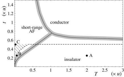
FIG. 1.: Crossover diagram of the half-filled 1D Hubbard model with Coulomb repulsion $U=2u$ and hopping $t$.

First, let us present the strong-coupling expansion itself. Consider a Hamiltonian ${\cal H}={\cal H}^{0}+{\cal H}^{1}$, where the unperturbed part ${\cal H}^{0}$ is diagonal in a certain variable $i$ (say a site variable), and let us denote collectively by ${\sigma}$ (say a spin variable) all the other variables of the problem. This Hamiltonian involves fermions, and is supposed to be normal ordered in terms of the annihilation and creation operators $c_{i{\sigma}}^{({\dagger})}$. ${\cal H}^{0}$ may be written as a sum over $i$ of on-site Hamiltonians involving only the operators $c_{i{\sigma}}^{({\dagger})}$ at site $i$: ${\cal H}^{0}=\sum_{i}h_{i}(c_{i{\sigma}}^{{\dagger}},c_{i{\sigma}})\>.$ For a strong-coupling expansion of the HM, ${\cal H}^{0}$ is the atomic limit, namely $h_{i}(c_{i{\sigma}}^{{\dagger}},c_{i{\sigma}})=Uc_{i{\uparrow}}^{{\dagger}}c_{i{\downarrow}}^{{\dagger}}c_{i{\downarrow}}c_{i{\uparrow}}\>$ (we will often use $u=U/2$ for convenience). We suppose that the perturbation ${\cal H}^{1}$ is a one-body operator of the form ${\cal H}^{1}=\sum_{\sigma}\sum_{ij}V_{ij}c_{i{\sigma}}^{{\dagger}}c_{j{\sigma}}\>$. For the HM, ${\cal H}^{1}$ is the kinetic term. Introducing the Grassmann field ${\gamma}_{i{\sigma}}(\tau),{\gamma}_{i{\sigma}}^{\star}(\tau)$, the partition function at some temperature $T=1/{\beta}$ may be written in the Feynman path-integral formalism:

$$Z = \int[d{\gamma}^{\star}d{\gamma}]\exp-\int_{0}^{{\beta}}d\tau\Bigg{\{}\sum_{i{\sigma}}{\gamma}_{i{\sigma}}^{\star}(\tau)\left({\partial\over\partial\tau}-\mu\right){\gamma}_{i{\sigma}}(\tau)$$ (2)

$$+\sum_{i}h_{i}({\gamma}_{i{\sigma}}^{\star}(\tau),{\gamma}_{i{\sigma}}(\tau))+\sum_{ij{\sigma}}V_{ij}{\gamma}_{i{\sigma}}^{\star}(\tau){\gamma}_{j{\sigma}}(\tau)\Bigg{\}}\>.$$

We use the letters ($a,b,...$) to denote sets such as $(i,{\sigma},\tau)$, for instance :

$$\int_{0}^{{\beta}}d\tau\sum_{ij{\sigma}}V_{ij}{\gamma}_{i{\sigma}}^{\star}(\tau){\gamma}_{j{\sigma}}(\tau)=\sum_{ab}V_{ab}{\gamma}_{a}^{\star}{\gamma}_{b}\>.$$ (3)

A first difficulty arises: There is no Wick theorem because ${\cal H}^{0}$ is quartic instead of quadratic. We solve this problem by means of a Grassmannian Hubbard-Stratonovich transformation, [22] which consists in expressing the perturbation part of the action in Eq. (2) as a Gaussian integral over an auxiliary Grassmann field $\psi_{i{\sigma}}(\tau),\psi_{i{\sigma}}^{\star}(\tau)$. Then, the integral over the original variables can be performed and $Z$ can be rewritten in the form:

$$Z=\int[d\psi^{\star}d\psi]\exp-\left\{S_{0}[\psi^{\star},\psi]+\sum_{R=1}^{\infty}S_{\rm int}^{R}[\psi^{\star},\psi]\right\}\>.$$ (4)

The action has a free part

$$S_{0}[\psi^{\star},\psi]=-\sum_{ab}\psi^{\star}_{a}\left(V^{-1}\right)_{ab}\psi_{b}\>,$$ (5)

and an infinite number of interaction terms

$$S_{\rm int}^{R}[\psi^{\star},\psi]={-1\over(R!)^{2}}\sum_{\{a_{l},b_{l}\}}{}^{\prime}\psi_{a_{1}}^{\star}..\psi_{a_{R}}^{\star}\psi_{b_{R}}..\psi_{b_{1}}G^{R\rm c}_{\scriptstyle a_{1}..a_{R}\atop\scriptstyle b_{1}..b_{R}},$$ (6)

where the $G^{R\rm c}_{\scriptstyle a_{1}..a_{R}\atop\scriptstyle b_{1}..b_{R}}={\left\langle{\gamma}_{a_{1}}..{\gamma}_{a_{R}}{\gamma}_{b_{R}}^{\star}..{\gamma}_{b_{1}}^{\star}\right\rangle}_{0,{\rm c}}$ are the connected correlation functions of the unperturbed system. The primed summation reminds us that the fields in each term share the same value of the site index. We may now use Wick’s theorem and usual perturbation theory for the $\psi$’s, the free propagator being $V$, and the vertices being the $G^{R\rm c}$’s. The number of auxiliary field propagators determines the order in $V$ ($|V_{ij}|=t$ for the HM) of a given diagram. Finally, the relation between the Green function ${\cal G}_{ab}=-{\left\langle{\gamma}_{a}{\gamma}_{b}^{\star}\right\rangle}$ of the original fermions and that of the auxiliary field ${\cal V}_{ab}=-{\left\langle\psi_{a}\psi_{b}^{\star}\right\rangle}$, is (in matrix form) ${\cal G}=-V^{-1}+V^{-1}{\cal V}V^{-1}\>.$ If ${\Gamma}$ denotes the self-energy of the $\psi$’s, one has ${\cal G}=\left({\Gamma}^{-1}-V\right)^{-1}\>.$

The above method was applied to the HM

$${\cal H}=2u\sum_{i}c_{i{\uparrow}}^{{\dagger}}c_{i{\downarrow}}^{{\dagger}}c_{i{\downarrow}}c_{i{\uparrow}}-t\sum_{\left\langle i,j\right\rangle{\sigma}}(c_{i{\sigma}}^{{\dagger}}c_{j{\sigma}}+{\rm H.c.})$$ (7)

at half-filling up to order $t^{3}$. The result for ${\cal G}$ is a rational function of ${i{\omega}_{n}}$:

$${1\over{\cal G}({\bf k},{i{\omega}_{n}})}=2tc({\bf k})+\Bigg{\{}{{i{\omega}_{n}}\over({i{\omega}_{n}})^{2}-u^{2}}+{6dt^{2}u^{2}{i{\omega}_{n}}\over\left(({i{\omega}_{n}})^{2}-u^{2}\right)^{3}}$$ (8)

$$+6t^{3}c({\bf k})\left({{{\beta}u\over 2}\tanh{\left({{\beta}u\over 2}\right)}\over\left(({i{\omega}_{n}})^{2}-u^{2}\right)^{2}}+{u^{2}\left(2({i{\omega}_{n}})^{2}-u^{2}\right)\over\left(({i{\omega}_{n}})^{2}-u^{2}\right)^{4}}\right)\Bigg{\}}^{-1},$$ (9)

where $d$ is the dimension of the hypercubic lattice, and $c({\bf k})=\sum_{m=1}^{d}\cos(k_{m})$. Here we face a second difficulty, namely that ${\cal G}({\bf k},{i{\omega}_{n}})$ has pairs of complex conjugate poles. This violates the Kramers-Krönig relations and leads to negative spectral weight. Note that even in weak-coupling theory, truncation of the series for ${\cal G}$ leads to high-order poles giving negative spectral weight. Since we only know ${\cal G}$ up to order $t^{3}$, any function having the same Taylor expansion as ${\cal G}$ to this order is a priori as good an approximation. A physically acceptable solution should be causal and have a positive spectral weight, that is, be a sum of simple real poles with positive residues. We call such a function Lehmann representable (LR).

In order to obtain a LR approximation, we need the following theorem, reported in Ref. [23]: A rational function is LR if and only if it can be written as a finite Jacobi continued fraction

$${\cal G}_{J}({i{\omega}_{n}})={a_{0}\over{i{\omega}_{n}}+b_{1}-}\>{a_{1}\over{i{\omega}_{n}}+b_{2}-}\>...\>{a_{L-1}\over{i{\omega}_{n}}+b_{L}}\>,$$ (10)

with $b_{l}$ real and $a_{l}>0$ (thereafter conditions CO).

According to this theorem, the exact Green function of any finite system is a Jacobi continued fraction, whose coefficients, functions of the hopping $t$, verify conditions CO. If we expand the exact ${\cal G}_{J}$ in powers of $t$ to some finite order, which is what a strong-coupling expansion does, we destroy its continued fraction structure. If instead we replace $a_{l}(t)$ and $b_{l}(t)$ in ${\cal G}_{J}$ by their expansion to some finite order, the result should be LR since we expect conditions CO to hold for the truncated coefficients (at least for $t/u$ small).

Therefore, to obtain a LR approximation, we seek frequency-independent $a_{l}(t)$ and $b_{l}(t)$, such that ${\cal G}_{J}$ and $\cal G$ have the same expansion up to order $t^{3}$. Equating the series in $t$ for $\cal G$ and for ${\cal G}_{J}$ at all frequencies determines uniquely the leading terms in the $t$ expansion of $a_{l}(t)$ and $b_{l}(t)$. As soon as some $a_{l}(t)$ is found to be zero up to the required precision necessary to obtain the $t^{3}$ term of ${\cal G}_{J}$, all $a_{p}(t)$ and $b_{p}(t)$, $p>l$ become unecessary.

The above procedure generalizes what is done in weak-coupling theory. There, Wick’s theorem allows a resummation of one-particle reducible diagrams, which gives Dyson’s equation. If the self-energy is LR, (i.e., has an underlying continued fraction structure), the Green function inherits this property due to the form of the weak-coupling free propagator.

We were able to deduce from Eq. (8) the following continued fraction

$${\cal G}_{J}({i{\omega}_{n}}) = {1\over{i{\omega}_{n}}+2tc({\bf k})-}\>{u^{2}\over{i{\omega}_{n}}-{3{\beta}t^{3}}\tanh{\left({{\beta}u\over 2}\right)}c({\bf k})/u-}$$ (12)

$${6dt^{2}\over{i{\omega}_{n}}-2tc({\bf k})/d-}\>{u^{2}\over{i{\omega}_{n}}+tc({\bf k})/d}\>,$$

which verifies the conditions CO, and has exactly the same Taylor expansion as $\cal G$ up to order $t^{3}$ included. This means that all the moments[24] of ${\cal G}_{J}$ are the same as those of the exact solution except for terms of order $t^{4}$. Furthermore, any LR rational function sharing this property reduces to a continued fraction whose coefficients differ from those of Eq. (12) only by terms smaller than the precision achieved here [25].

Expansion to order $t^{3}$ for the half-filled HM suffices to exhibit both the Mott transition and the effect of AF correlations on the spectral weight $A({\bf k},{\omega})=\lim_{\>\eta\rightarrow 0^{+}}-2\>{\rm Im}\>{\cal G}({\bf k},{\omega}+i\eta)$. There is no rigorous definition of the Mott transition in terms of one-particle properties, but one can use, as a heuristic criterion, the appearance of spectral weight at zero frequency. In the density of states $N({\omega})=\int_{-\pi}^{\pi}A({\bf k},{\omega})d^{d}{\bf k}/(2\pi)^{d}$, as $t$ increases from zero, the two symmetric Hubbard bands located at $u$ and $-u$ in the atomic limit widen, and eventually mix for $t$ beyond some critical value. The latter may be obtained by demanding that a pole of $\cal G$ crosses the Fermi level for some ${\bf k}$. For $T\rightarrow\infty$, the critical value of $t$ is $t_{\rm c}=u{\sqrt{1+\sqrt{1+12d^{2}}}/(2d\sqrt{3}})$ [26]. This gives $U_{\rm c}\simeq 3.2t$ for $d=1$, to be compared with $U_{\rm c}\simeq 3.5t$ found in the Hubbard-III[4] approximation. At finite $T$, we cannot calculate $t_{\rm c}$ analytically, but Fig. 1 sketches a numerical evaluation (for $d=1$) in the ($T,t$) plane of the line where the gap vanishes. The value of $t_{\rm c}$ grows upon lowering $T$, and there is no Mott transition at zero temperature, in agreement with the exact result of Ref. [5].

The effects of AF correlations show up at low T, as illustrated in Fig. 2 by the plot of $A(k,\omega)$ for point B of Fig. 1 ($\bf k$ becomes $k$ because we discuss the 1D case for definiteness). $A(k,{\omega})$ has four delta peaks (a finite width $\eta$ is added for clarity) given by dispersion relations ${\omega}_{i}(k)$, ($i$=1 to 4 as in Fig. 2). The spectral weight is an even function of $k$, and particle-hole symmetry ensures that $A(k+\pi,-{\omega})=A(k,{\omega})$. While at small $t$ and high $T$ (point A), $\omega_{2}(k)$ was minimum for $k=0$, when $T$ is lowered down to point B, the minimum of $\omega_{2}(k)$ moves continuously from $k=0$ towards $k=\pi/2$ (Fig. 2), and peak 2 loses weight for values of $k$ much smaller than $\pi/2$. These changes reflect the AF short-range order that gradually builds up when $T$ becomes smaller than the AF superexchange $J=2t^{2}/u$ of the equivalent $t-J$ model. The approximate cell doubling in direct space translates into a nearly $\pi$-periodic dispersion for peak 2, although the $2\pi$-periodicity of its weight and of ${\omega}_{1}(k)$ reminds us that the state remains paramagnetic. This is why we chose to define the AF crossover line of Fig. 1 as the points where $k=0$ ceases to be the minimum of ${\omega}_{2}(k)$. In this regime, the width of band 2 is of order $J=2t^{2}/u$ whatever the value of $t$, supporting the above interpretation.

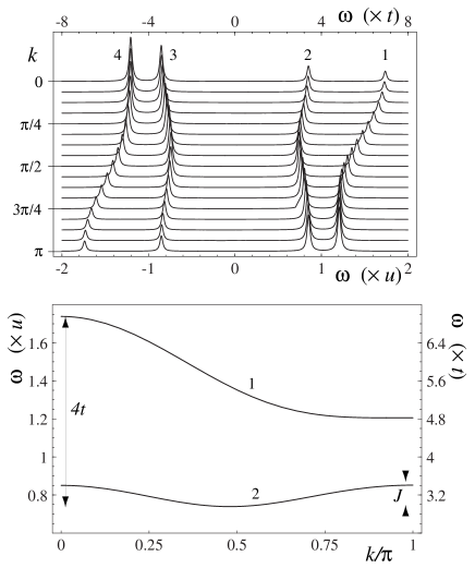
FIG. 2.: (above) Spectral function $A(k,{\omega})$ for point B ($t=0.25u,\>T=0.06u$ or $U=8t,\>T=0.24t$). $\eta$ (see text) was set to $0.02$. (below) Dispersion relation of the peaks.

If we decrease T further from point B, we enter a regime that is beyond the domain of validity of our approach. Indeed, in contradiction with the results of Refs. [12, 9, 3], the spectral function becomes similar to that of free particles, following a $-2t\cos k$ dispersion, except for a gap at the Fermi energy for $k\simeq\pi/2$. We expect our expansion to be valid if the $b_{l}(t)$’s in Eq. (12) are small compared to ${\omega}$, whose lowest-order value is $u$. This leads us to the conditions $t/u\lesssim 0.5$ and $3(t/u)^{3}\lesssim T/u$, fulfilled by the points under the dashed line in Fig. 1. However, these conditions may be too stringent because the $t\rightarrow\infty$ limit also happens to be correctly given by our solution Eq. (12). Furthermore, a free particle dispersion relation, with a gap opened at the Fermi level, is what is expected at large $t$ and small $T$ for an itinerant antiferromagnet. Fig. 3 (point C) illustrates this behaviour. The parameters have the same value as in the Monte-Carlo (MC) calculations of Ref. [6] ($U=4t$, ${\beta}=20/t$). The general distribution of the spectral weight, and the dispersion relation of the peaks [6] are well accounted for by our solution. We believe that peak 1 contributes to the large uncertainty (due mainly to the Maximum Entropy Method itself) on the maxima of $A(k,{\omega})$ reported in Fig. 2 of Ref. [6] for $k$ near $0$ and $\pi$. For other values of $k$, peak 1 could not be resolved in Ref. [6] because of its small weight and because of the magnitude of the time slice, unlikely to detect high-energy features. Thus, our results for point C appear correct. Our method definitely fails in the shaded area of Fig. 1, where spin-charge separation occurs, but outside this region our solution is reliable under the dashed line, and uncontrolled (but not necessarily bad) above it.

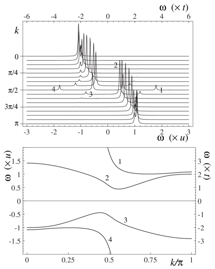
FIG. 3.: (above) Spectral function $A(k,{\omega})$ for point C ($t=0.5u,\>T=0.025u$ or $U=4t,\>T=0.05t,\>{\beta}=20/t$) with $\eta=0.02$. (below) Dispersion relation of the peaks.

The cuprate chain material $\rm SrCuO_{2}$ studied in Ref. [3] happens to fall in the shaded regime. Nevertheless, our results allow us to predict that features dispersing on a scale $J$, like peak 3 in Fig. 2, should appear at $\pi/2\leq k\leq\pi$ upon raising T. Hints of this finite T effect have already been seen in the “question-mark” features in Fig. 1 of Ref. [3].

In summary, we presented a general method for constructing strong-coupling expansions and applied it to the half-filled Hubbard model. We showed how the Mott transition and AF correlations manifest themselves in the single-particle properties. Finally, we gained further insight into ongoing ARPES experiments on the propagation of one hole in an AF correlated Mott insulator. Doping and two-particle correlations are accessible within the same approach.

We thank C. Bourbonnais for numerous enlightening discussions. We are also grateful to H. Touchette, L. Chen and S. Moukouri for sharing their numerical results. This work was partially supported by NSERC (Canada), by FCAR (Québec), by a scholarship from MESR (France) to S.P. and (for A.-M.S.T.) by the Canadian Institute for Advanced Research.

REFERENCES

- [1] Also at the Laboratoire de Physique des Solides, Université Paris-Sud, 91405, Orsay, France.
- [2] B. O. Wells et al, Phys. Rev. Lett. 74, 964 (1995).
- [3] C. Kim et al, Phys. Rev. Lett. 77, 4054 (1996).
- [4] J. Hubbard, Proc. R. Soc. (London) Ser. A 276, 238 (1963), A 277, 237 (1964), A 281, 401 (1964), A 285, 542 (1965).
- [5] E. H. Lieb, F. Y. Wu, Phys. Rev. Lett. 20, 1445 (1968).
- [6] R. Preuss et al, Phys. Rev. Lett. 73, 732 (1994) and Ref.[14] therein.
- [7] R. Preuss, W. Hanke, W. von der Linden, Phys. Rev. Lett. 75, 1344 (1995).
- [8] N. Bulut, D. J. Scalapino, S. R. White, Phys. Rev. B 50, 7215 (1994).
- [9] J. Favand et al, Phys. Rev. B 55, R4859 (1997).
- [10] V. J. Emery, in Highly Conducting One- Dimensional Solids, 247, by J. T. Devreese et al, Plenum (1979).
- [11] J. Voit, Rep. Prog. Phys. 57, 977 (1994).
- [12] J. Voit, cond-mat/9711064 (1997).
- [13] J. Sólyom, Adv. Phys. 28, 201 (1979).
- [14] C. Bourbonnais, L. G. Caron, Int. J. Mod. Phys. B 5, 1033 (1991).
- [15] H. Frahm, V. E. Korepin, Phys. Rev. B 42, 10553 (1990); Phys. Rev. B 43, 5653 (1991).
- [16] W. Metzner, D. Vollhardt, Phys. Rev. Lett. 62, 324 (1989). M. J. Rozenberg, X. Y. Zhang, G. Kotliar, Phys. Rev. Lett. 69, 1236 (1992). A. Georges, W. Krauth, Phys. Rev. Lett. 69, 1240 (1992).
- [17] A. Georges, W. Krauth, Phys. Rev. B 48, 7167 (1993).
- [18] Th. Pruschke, D. L. Cox, M. Jarell, Phys. Rev. B 47, 3553 (1993).
- [19] A. Georges et al, Rev. Mod. Phys. 68, 13 (1996).
- [20] M. Bartkowiak, K. A. Chao, Phys. Rev. B 46, 9228 (1992).
- [21] W. Metzner, Phys. Rev. B 43, 8549 (1991).
- [22] C. Bourbonnais, PhD thesis, Université de Sherbrooke, (1985). D. Boies, C. Bourbonnais, A.-M. S. Tremblay, Phys. Rev. Lett. 74, 968 (1995). S.K. Sarker, J. Phys. C: Solid State Phys. 21, L667 (1988) ( the latter reference was pointed out to us by R. Frésard).
- [23] J. Gilewicz, Approximants de Padé, Lecture Notes in Mathematics 667, Springer-Verlag (1978).
- [24] We call the moments of the spectral function.
- [25] difference in for , for , for all other coefficients.
- [26] This simple criterion yields (with ) in infinite dimension. This critical value of interaction strength is too large because when our criterion corresponds to subbands that meet with an exponentially small density of states, therefore not yet truly closing the gap.