Alternating Kinetics of Annihilating Random Walks Near a Free Interface

Abstract

The kinetics of annihilating random walks in one dimension, with the half-line $x>0$ initially filled, is investigated. The survival probability of the $n^{\rm th}$ particle from the interface exhibits power-law decay, $S_{n}(t)\sim t^{-\alpha_{n}}$, with $\alpha_{n}\approx 0.225$ for $n=1$ and all odd values of $n$; for all $n$ even, a faster decay with $\alpha_{n}\approx 0.865$ is observed. From consideration of the eventual survival probability in a finite cluster of particles, the rigorous bound $\alpha_{1}\leq 1/4$ is derived, while a heuristic argument gives $\alpha_{1}\approx 3\sqrt{3}/8=0.2067\ldots$. Numerically, this latter value appears to be a lower bound for $\alpha_{1}$. The average position of the first particle moves to the right approximately as $1.7\,t^{1/2}$, with a relatively sharp and asymmetric probability distribution.

PACS numbers: 02.50.Ga, 05.70.Ln, 05.40.+j

Annihilating random walks (ARWs) represent a simple but ubiquitous reaction process in which particles diffuse and annihilate whenever they meet[1]. In addition to providing general insights about non-equilibrium phenomena, ARWs underlie a variety of basic kinetic processes ranging from the voter model[2] and the kinetic Ising-Glauber model[3], to reaction-diffusion systems[4] and wetting phenomena[5]. In one dimension, powerful exact solution methods have been developed to understand many kinetic and spatial properties of ARWs[6, 7, 8, 9, 10, 11].

While much is known about ARWs under homogeneous conditions, the role of spatial heterogeneity in such non-equilibrium systems is relatively unexplored. Our particular interest is to understand the influence of a free interface on the asymptotic behavior of ARWs. For equilibrium systems at criticality, the presence of such a free interface gives rise to well understood surface critical behavior which is characterized by associated surface critical exponents[12, 13]. For reactive systems, in contrast, while there has been some progress in understanding the role of heterogeneity in the intrinsic properties of the reactants[14, 15, 16, 17, 18], the role of heterogeneity in the form of a free interface is still unexplored.

In this paper, we investigate basic properties of a one-dimensional semi-infinite system of ARWs. We consider a linear chain in which one particle initially occupies each lattice site $n$ for $n>0$, while the system is empty for $n\leq 0$. Far from the interface, the behavior should coincide with that of the homogeneous system. However, the interfacial region is a less reactive environment because one side of the system is initially empty. One might thus anticipate that particles near the interface should exhibit slower kinetics and different spatial properties than bulk particles. This expectation is only partly correct; in fact, every other particle near the interface exhibits faster kinetics compared to bulk particles. Our work further indicates that there are only two apparently independent “surface” exponents which characterize the asymptotic particle survival probabilities. This surface behavior eventually governs the entire system, although it penetrates slowly into the bulk by diffusion.

To quantify the phenomena that are governed by the existence of the interface in the semi-infinite ARW system, our work is organized around the following basic questions:

• What is the probability that the first particle survives until time $t$, $S_{1}(t)$? More generally, what is the survival probability for the $n^{\rm th}$ particle from the interface, $S_{n}(t)$?

• What is the probability that particles $i$ and $j$ react as a function of $|i-j|$ (with $i=1$ or 2 and $j$ arbitrary)?

• What is the spatial density distribution near the interface?

To answer the first question, let us introduce the exponents $\alpha_{n}$ to characterize the probability that the $n^{\rm th}$ particle survives until time $t$, $S_{n}(t)\sim t^{-\alpha_{n}}$. We first argue that there are only two independent exponents – one for $n$ odd and a second for $n$ even. To support this assertion, it is instructive to examine finite particle systems. For 3 particles, the first and third particles have a finite probability to survive indefinitely, while the second certainly dies, with a survival probability which decays as $t^{-3/2}$[10, 19, 20]. Similar asymptotic behavior can be anticipated for all finite systems with an odd number of particles. In such cases, the asymptotically dominant contribution to $S_{n}(t)$ for $n$ even will come from 3-particle configurations where an even particle is between two odd particles, with all other particles already annihilated. Conversely, particles with odd labels have a finite probability to survive indefinitely. Thus for the finite-particle system $\alpha_{n}=0$ for $n$ odd and $\alpha_{n}=3/2$ for $n$ even. On this basis, we anticipate that just two exponents also characterize the individual particle survival probabilities in the semi-infinite system.

To test these predictions, we performed numerical simulations using two complementary methods. The first (naive) approach is to simulate a suitably-sized system with the initial condition that the right half-line is completely occupied while the left half-line is empty. Reflecting boundary conditions are employed at the edges of the system. The system size is chosen such that the effect of the boundaries is negligible over the time scale of the simulation. In the second approach, particles are created at the right boundary at a rate equal to the exact time-dependent density of the homogeneous system, $c(t)\simeq(4\pi t)^{-1/2}$[6, 10], to mimic the effect of a semi-infinite system. This is a more efficient approach, as relatively long-time simulations can be run on a small systems without being influenced by boundary effects. For the survival probability of the first particle our simulations give $S_{1}(t)\sim t^{-\alpha_{1}}$, with $\alpha_{1}=0.225\pm 0.005$. On the other hand, for the second particle, $S_{2}(t)\sim t^{-\alpha_{2}}$ with $\alpha_{2}=0.865\pm 0.015$. As anticipated, the survival probability of the first particle ($n=1$) decays more slowly than $t^{-1/2}$, the particle survival probability in the bulk. However, the second particle is much less likely to survive than a bulk particle. This arises because the second particle always has a unique potential left reaction partner, as well as a right reaction partner.

FIG. 1.: Simulation results for $S_{1}(t)$ ($\circ$) and $S_{2}(t)$ ($\Delta$). The quoted exponents are based on the best-fit straight lines to the data given in the figure.

To determine whether the survival probabilities $S_{n}(t)$ are characterized by only two exponents, we perform a scaling analysis. Particles far from the interface initially exhibit bulk behavior, where $S_{n}(t)\sim t^{-1/2}$ for all $n$. After a time $t_{n}\sim n^{2}$, the $n^{\rm th}$ particle “senses” the interface, and crossover from bulk to surface kinetics should occur. Based on the observed asymptotic behavior of $S_{1}(t)$ and $S_{2}(t)$, together with the above crossover picture, we expect that $S_{n}(t)$ should exhibit the two distinct scaling forms for odd and even $n$ respectively,

$$S_{2n-1}(t)\simeq t^{-1/2}{\cal O}(z),\quad S_{2n}(t)\simeq t^{-1/2}{\cal E}(z),$$ (1)

for $t\rightarrow\infty$ and $n\rightarrow\infty$, with $z=nt^{-1/2}$ finite. Large values of $z$ corresponds to particles sufficiently deep in the bulk that they are not yet influenced by the heterogeneous initial condition. Thus the large argument behavior of the scaling functions is determined by the survival probability of the homogeneous system. Since $S(t)=c(t)\simeq(4\pi t)^{-1/2}$[6, 10], this gives ${\cal O}(\infty)={\cal E}(\infty)=1/\sqrt{4\pi}$. Conversely, for $z\ll 1$

$${\cal O}(z)\sim z^{\mu_{1}},\quad{\cal E}(z)\sim z^{\mu_{2}},$$ (2)

with $\mu_{1}=2\alpha_{1}-1$ and $\mu_{2}=2\alpha_{2}-1$ to match with the long time behavior of $S_{1}(t)$ and $S_{2}(t)$. As Figure 2 shows, $S_{n}(t)$ follows this general description.

FIG. 2.: Simulation results for the time dependence of the survival probability of the $n^{\rm th}$ particle, $S_{n}(t)$, for $1\leq n\leq 100$. Shown are the scaling functions ${\cal O}(z)$ (upper curve) and ${\cal E}(z)$ (lower) versus $z=nt^{-1/2}$ at $t=16$ ($\circ$), 256 ($\Box$), and 4096 ($\Delta$). For large $z$, both scaling functions approach the limiting value $(4\pi)^{-1/2}\approx 0.2821$.

We can provide a relatively tight rigorous upper bound for the exponent $\alpha_{1}$. We will also present a heuristic argument, based on an uncontrolled approximation, which turns out to give a relatively stringent lower bound for $\alpha_{1}$. For both situations, our approach is based on first finding the ultimate survival probability of the first particle in a finite-particle system on an infinite lattice and then using scaling to infer time dependence, from which bounds on $\alpha_{1}$ can be inferred. Let the particles be initially distributed on $N$ adjacent lattice sites, with $N$ odd. Ultimately, a unique particle survives which could be the first, the third, the fifth, etc., in the initial sequence. Let ${\cal S}_{1}(N)$ be the probability that the first particle is this unique survivor. For $N\to\infty$, we shall show that this probability scales as

$${\cal S}_{1}(N)\sim{1\over N^{2\beta_{1}}}.$$ (3)

On the other hand, for $t<N^{2}$, the finiteness of the system is immaterial and the survival probability of the first particle should coincide with $S_{1}(t)$ in the semi-infinite system. When $t$ becomes of the order of $N$, the number of particles remaining will be of order unity and $S_{1}(t)$ should “stick” at the value ${\cal S}_{1}(N)$. Thus substituting $t^{1/2}$ for $N$ in Eq. (3) and equating to $S_{1}(t)$ gives $\beta_{1}=\alpha_{1}$.

First consider an upper bound for $\alpha_{1}$. A naive approximation is to suppose that every collision between nearest-neighbors has the same probability to occur. For the initial $N$ particles there are $N-1$ collision possible and the probability that the first particle survives after the first collision is $(N-2)/(N-1)$. This leaves $N-2$ particles and $N-3$ possible collisions, and the probability that the first particle survives after this second collision is $(N-4)/(N-3)$. The ultimate survival probability of the first particle in this “democratic” approximation is

$${\cal S}_{1}^{D}(N) = {(N-2)(N-4)\ldots 3\times 1\over(N-1)(N-3)\ldots 4\times 2}$$ (4)

$$\sim \sqrt{2\over{\pi N}}\quad N\to\infty.$$ (5)

However ${\cal S}_{1}(N)\geq{\cal S}_{1}^{D}(N)$, because the first particle has the possibility to “escape” on its empty side, and therefore collisions involving this particle are relatively less likely. Thus we conclude[21]

$$\alpha_{1}\leq 1/4.$$ (6)

While we are unable to obtain a rigorous lower bound for $\alpha_{1}$, we have a heuristic approach that gives ${\cal S}_{1}(N)\sim N^{-\gamma}$, with $\gamma=3\sqrt{3}/4\pi$. This approach is based on first recasting the annihilation problem into an equivalent aggregation process[10]. In aggregation, point-like $k$-mers perform random walks with a mass-independent diffusion coefficient. When two polymers of masses $i$ and $j$ happen to occupy the same site, they irreversibly aggregate into a heavier but still point-like polymer of mass $i+j$, as represented by the reaction scheme

$$A_{i}+A_{j}\rightarrow A_{i+j}.$$ (7)

To make the connection with annihilation, we categorize polymers according to whether their mass is odd, $A_{o}=\{A_{1},A_{3},\ldots\}$, or even, $A_{e}=\{A_{2},A_{4},\ldots\}$, respectively. These two classes of polymers react according to

$$A_{e}+A_{e} \rightarrow A_{e},$$ (8)

$$A_{o}+A_{e} \rightarrow A_{o},$$ (9)

$$A_{o}+A_{o} \rightarrow A_{e}.$$ (10)

In particular, the parity of odd-mass polymers is not influenced by even-mass polymers. Thus by considering only odd-mass polymers, aggregation is completely equivalent to ARW[10].

If one associates the initial particles in ARW with monomers in aggregation, then the first particle survives in the ARW process if the mass of the leftmost polymer in the corresponding aggregation process remains odd throughout the evolution. With this equivalence, we now postulate, in the spirit of a Kirkwood approximation, that ${\cal S}_{1}(N)$ obeys the recursion relation

$${\cal S}_{1}(N+2)\approx{\cal S}_{1}(N)F(N+2)\approx\prod_{\stackrel{{\scriptstyle k=1}}{{k~{}{\rm odd}}}}^{N+2}F(k).$$ (11)

Here $F(k)$ is the probability that the first collision between three random walks, which are initially at $x_{0}=1$, $y_{0}=k-1$, and $z_{0}=k$, occurs between the particles at $k-1$ and $k$. While this approximation is uncontrolled, it turns out to give a relatively stringent upper bound for the true behavior of ${\cal S}_{1}(N)$ (see Fig. (3)).

To compute $F(k)$, we map the problem of three random walks, initially at $x_{0}$, $y_{0}$, and $z_{0}$ in one dimension, onto a single random walk in three dimensions[19, 20]. A collision between particles 1 and 2, and between 2 and 3 imposes the boundary conditions that the probability distribution vanishes when $x=y$ and $y=z$, respectively. This implies that the three-dimensional walk is confined to the wedge-shaped region defined by $x\leq y$ and $y\leq z$. Using image techniques, the probability distribution in the continuum limit can be written down, from which the desired eventual collision probability follows after some tedious calculation.

For simplicity, we give an alternative derivation which exploits the isomorphism between the eventual collision probability and electrostatics[22]. The three-dimensional region $x\leq y$ and $y\leq z$ can be projected into two dimensions, with the allowed region now a wedge of opening angle $\Omega=\pi/3$[19, 20]. Any initial state of three random walks maps to a point in this two-dimensional domain. To determine the co-ordinates of this initial point, we need to define a two-dimensional co-ordinate system which is perpendicular to the axis $\hat{e}_{1}=(1,1,1)/\sqrt{3}$ generated by the intersection of the planes $x=y$ and $y=z$. A convenient basis is $\hat{e}_{2}=(0,-1,1)/\sqrt{2}$ and $\hat{e}_{3}=(-2,1,1)/\sqrt{6}$. The initial condition $\vec{r}_{0}=(x_{0},y_{0},z_{0})$ has components $d_{2}=\vec{r}_{0}\cdot\hat{e}_{2}=(z_{0}-y_{0})/\sqrt{2}$ and $d_{3}=\vec{r}_{0}\cdot\hat{e}_{3}=(-2x_{0}+y_{0}+z_{0})/\sqrt{6}$ in the $\hat{e}_{2}$ and $e_{3}$ basis. Within the two-dimensional wedge, with the horizontal axis defined as the locus where $y=z$, an arbitrary initial condition corresponds to a horizontal displacement of $(z_{0}+y_{0}-2x_{0})/\sqrt{6}$ and a vertical displacement of $(z_{0}-y_{0})/\sqrt{2}$. Thus the initial point is inclined at an angle

$$\theta=\tan^{-1}{d_{2}\over d_{3}}=\tan^{-1}\left[\sqrt{3}\left({{z_{0}-y_{0}}\over{z_{0}+y_{0}-2x_{0}}}\right)\right]$$ (12)

with respect to the horizontal.

We want to compute the probability that the random walk eventually hits the horizontal axis, corresponding to particles 2 and 3 colliding. From the isomorphism with electrostatics, this probability equals the integral of the electric field over the horizontal axis, which is generated by the unit charge at the initial position of the random walk[22]. To simplify computation of this integral, perform the conformal transformation $w=z^{3}$ to open the wedge onto the upper half plane, so that the initial point is now inclined at an angle $3\theta$ with respect to the positive real axis. In real co-ordinates, for an initial point at $(x_{0},y_{0})$ with a grounded plane at $y=0$, the electric field at $(x,0)$ equals

$${y_{0}\over\pi}{1\over{(x-x_{0})^{2}+y_{0}^{2}}}.$$ (13)

The integral of this field over any interval on the $x$-axis gives the probability that a random walk which starts at ($x_{0},y_{0}$) eventually hits this interval. This gives ${\phi\over\pi}$, where $\phi$ is the angular size of the interval as seen from the location of the charge. In our case the appropriate interval $x=(0,\infty)$ has angular size $\phi=\pi-3\theta$, so that

$$F(k) = 1-{3\theta\over\pi}$$ (14)

$$= 1-{3\over\pi}\tan^{-1}{\sqrt{3}\over 2k-3}$$ (15)

$$\to 1-{3\sqrt{3}\over 2\pi k},\qquad k\to\infty,$$ (16)

where the second line is obtained by the substitution of the initial condition $x_{0}=1$, $y_{0}=k-1$, and $z_{0}=k$, as specified by the definition of $F(k)$. Note that this result is easily generalizable to the case where the three particles have distinct diffusivities.

FIG. 3.: Simulation results for the probability that the first particle ultimately survives from among an initial group of $N$ adjacent particles (with $N$ odd) on an infinite chain. The lower curve represents the rigorous bound given in Eq. (4), and the upper curve represents the heuristic bound from Eqs. (8) and (11).

Using Eq. (11), we obtain

$${\cal S}_{1}(N)\approx\prod_{\stackrel{{\scriptstyle k=1}}{{k~{}{\rm odd}}}}^{N}\left(1-{3\sqrt{3}\over{2\pi k}}\right)\sim N^{-3\sqrt{3}/4\pi}.$$ (17)

Thus we arrive at the following approximate expression for $\alpha_{1}$

$$\alpha_{1}={3\sqrt{3}\over 8\pi}\simeq 0.2067\ldots$$ (18)

Let us now consider the exponent $\alpha_{2}$. We write the survival probability of the second particle as $S_{2}(t)=P(t)S_{R}(t)$, where $P(t)\sim t^{-1/2}$ is the probability that the particle has not been annihilated by its single left neighbor and $S_{R}(t)$ is the probability that the particle has not been annihilated by any particle to its right. This latter probability decays as $t^{-1/4}$, since in the bulk the survival probability $S(t)=S_{L}(t)S_{R}(t)=S_{R}(t)^{2}$ varies as $t^{-1/2}$. This approximation immediately leads to $\alpha_{2}=3/4$ which can be expected to be the lower bound. Unfortunately, we have been unable to construct a non-trivial upper bound for $\alpha_{2}$. A trivial upper bound, however, is provided by the survival probability of the central particle in a 3-particle system. Consequently, we have the bounds

$${3\over 4}<\alpha_{2}<{3\over 2}.$$ (19)

We now turn to a related and useful microscopic characterization of the reaction process, namely, the probability that a particle is eventually annihilated by its n^th nearest-neighbor, $P(n)$[23]. For homogeneous reaction processes, $P(n)$ typically decays as a power law in $n$, $P(n)\sim n^{-\psi}$, and the exponent $\psi$ is related to the time dependence of the survival probability. For homogeneous ARWs, for example, the particle survival probability $S(t)$ decaying as $t^{-\alpha}$ (with $\alpha=1/2$) implies that the probability that a particle is annihilated at time $t$ is $-{dS(t)\over{dt}}\sim t^{-\alpha-1}$. The annihilation probabilities for given $t$ and $n$ can now be related by

$$-{dS(t)\over{dt}}\,dt=P(n)\,dn.$$ (20)

For diffusive transport, $n$ scales as $t^{1/2}$ and Eq. (20), together with the defining relations for $\alpha$ and $\psi$, then gives $\psi=1+2\alpha$.

We now apply the same line of reasoning for the semi-infinite system. Let us define the probability that the first particle is annihilated by the $n^{\rm th}$ particle as $P_{1}(n)\equiv n^{-\psi_{1}}$; our previous estimate for $\alpha_{1}$ gives $\psi_{1}=1+2\alpha_{1}\approx 1.45$. Similarly for the second particle, $P_{2}(n)\equiv n^{-\psi_{2}}$, with $\psi_{2}=1+2\alpha_{2}\approx 2.73$. As shown in Fig. 4, these expectations are consistent with our data. One additional interesting feature is that the second particle annihilates with the first particle with probability $\approx 0.5704$, while it annihilates with any other particle with probability $\approx 0.4296$.

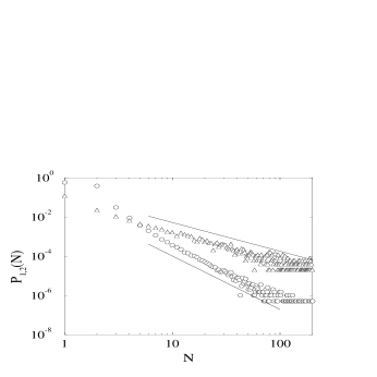
FIG. 4.: Simulation results for the annihilation probabilities $P_{1}(n)$ ($\circ$) and $P_{2}(n)$ ($\Delta$). For reference, the straight lines have slopes $-1.45$ and $-2.73$.

Finally, we study the spatial distribution of the leftmost particle. This refers to the extreme particle that currently exists and is not necessarily the initial particle that was leftmost. To provide some perspective on the behavior one might anticipate, first consider this question for two simpler systems with the same semi-infinite concentration profile, $c(x,t=0)=\Theta(x)$. For freely diffusing particles, the long time spatial distribution in the continuum limit is the error function, $c(x,t)={1\over 2}[1+{\rm erf}(x/\sqrt{4t})]$. From this, the concentration at $x=0$ remains fixed at the value 1/2, while the typical position of the leftmost particle is $x_{-}\approx-\sqrt{t\ln t}$. Thus freely diffusing particles substantially penetrate the negative half-line. For coalescing random walks, where particles react by $A+A\to A$, the leftmost particle simply undergoes free diffusion. Thus the concentration at $x=0$ vanishes as $t^{-1/2}$, while the typical position of the leftmost particle remains at the origin.

For ARWs, the concentration profile can be readily computed for arbitrary initial conditions from the direct correspondence to the Glauber solution of the kinetic Ising model[6]. This calculation gives

$$c(n,t) = {\rm e}^{-2t}\left[\sum_{m=0}^{\infty}(-1)^{n}I_{n+m}(t)\sum_{m=1}^{\infty}I_{n-m}(t)\right.$$ (22)

$$\qquad\qquad\left.+\sum_{m=0}^{\infty}I_{n+m}^{2}(t)\right].$$

This profile exhibits an overall $t^{-1/2}$ decay of the density and a non-trivial spatial dependence. In the long-time limit, the above expression can be reduced to the scaling form

$$c(n,t)=t^{-1/2}{\cal C}(z),$$ (23)

with $z=nt^{-1/2}$ and where the scaling function ${\cal C}(z)$ can be expressed in terms of single and double integrals of the error functions. While the computation of the density profile requires the knowledge of the two-point correlation function of the equivalent kinetic Ising model, the spatial distribution of the leftmost particle would require the knowledge of all the $n$-point correlation functions. Although it is in principle possible to obtain such functions [7], this is a considerable analytical task and we merely use simulations to provide numerical data for the spatial distribution of the leftmost particle, $P_{\rm left}(x,t)$ (Fig. 5). This distribution obeys the expected scaling behavior and is asymmetric in character, with the negative-$z$ tail decaying as $e^{-z^{2}}$ while the positive-$z$ tail decays as $e^{-z}$ with $z=xt^{-1/2}$. From this data, we find, for example, that the average position of the leftmost particle varies as $x_{\rm left}(t)\approx 1.7\,t^{1/2}$.

FIG. 5.: Simulation data for the probability distribution of the location of the leftmost particle. Shown is the scaled distribution $t^{1/2}P_{\rm left}(x,t)$ versus scaled co-ordinate $x/t^{1/2}$ for $t=16$ ($\circ$), 256 ($\Box$), and 4096 ($\Delta$).

In summary, we studied basic properties of a semi-infinite population of annihilating random walks near a free interface. Since particles near the interface have fewer potential reaction partners than bulk particles, these interface particles should be more long-lived than those in the bulk. This naive expectation turns out to be only partially correct. For the $n^{\rm th}$ particle from the interface (with $n=1$ corresponding to the particle at the interface), the survival probability $S_{n}(t)$ decays as $t^{-\alpha_{n}}$, with $\alpha_{n}\approx 0.225$ for all odd values of $n$, but $\alpha_{n}\approx 0.865$ for all even values of $n$. These exponents can be viewed as characterizing the surface critical behavior of ARWs in one dimension.

This alternating behavior stems from the fact that an odd particle can eventually become the leftmost particle in the system and hence be long-lived. Conversely, an even particle will always have potential reaction partners on both sides and therefore has a relatively shorter lifetime. For the odd particles, the bounds $3\sqrt{3}/8\pi\leq\alpha_{1}\leq 1/4$ were derived, with the lower bound non-rigorous but numerically accurate, by considering the eventual survival probability in a finite group of $N$ particles, with $N$ odd.

The relative longevity of the interface particle is also reflected in the fact that the mean position of its reaction partner drifts slowly to the right as $1.7\,t^{1/2}$. The functional form of the probability distribution of $x_{\rm left}$ could be obtained, in principle, from the $n$-point correlation functions of the equivalent kinetic Ising model; this appears to be a formidable and unenlightening task. The numerical data for $P_{\rm left}(x,t)$ clearly exhibits scaling and shows that the position of the leftmost particle is described by a single length scale which varies as $\sqrt{t}$.

We thank E. Ben-Naim, B. Derrida, and F. Leyvraz for helpful discussions. This research was supported in part by the Swiss National Foundation, the ARO (grant DAAH04-96-1-0114), and the NSF (grant DMR-9632059).

REFERENCES

- [1] See e.g., the collection of articles in Nonequilibrium Statistical Mechanics in One Dimension, edited by V. Privman (Cambridge University Press, New York, 1997).
- [2] T. M. Liggett, Interacting Particle Systems (Springer, New York, 1985).
- [3] See e.g. Ref. [1], reviews by Z. Racz, p. 73; N. Ito, p. 93; S. J. Cornell, p. 111; A. J. Bray, p. 143.
- [4] See e.g. Ref. [1], reviews by S. Redner, p. 3; D. ben-Avraham, p. 29; V. Privman, p. 167.
- [5] D. A. Huse and M. E. Fisher, Phys. Rev. B 29, 239 (1984); M. E. Fisher, J. Stat. Phys. 34, 667 (1984).
- [6] R. J. Glauber, J. Math Phys. 4, 294 (1963).
- [7] D. Bedeaux, K. E. Schuler and I. Oppenheim, J. Stat. Phys. 2, 1 (1970).
- [8] B. U. Felderhof, Rep. Math. Phys. 1, 215 (1970); 2, 151 (1971).
- [9] B. Derrida and R. Zeitak, Phys. Rev. E 54, 2513 (1996).
- [10] J. L. Spouge, Phys. Rev. Lett. 60, 871 (1988); B. R. Thomson, J. Phys. A 22, 879 (1989).
- [11] P. L. Krapivsky and E. Ben-Naim, Phys. Rev. E 56, 3788 (1997).
- [12] H. W. Diehl, in Phase Transitions and Critical Phenomena, vol. 10, edited by C. Domb and J. Lebowitz (Academic Press, London, 1983).
- [13] A. LeClair and A. W. W. Ludwig, hep-th/9708135 and references therein.
- [14] C. R. Doering, Physica A 188, 386 (1992).
- [15] B. Derrida, A. J. Bray, and C. Godrèche, J. Phys. A 27, L357 (1994).
- [16] P. L. Krapivsky, E. Ben-Naim, and S. Redner, Phys. Rev. E 50, 2474 (1994); C. Monthus, Phys. Rev. E 54, 4844 (1996).
- [17] B. Derrida, V. Hakim, and V. Pasquier, Phys. Rev. Lett. 75, 751 (1995).
- [18] E. Ben-Naim, L. Frachebourg, and P. L. Krapivsky, Phys. Rev. E 53, 3078 (1996).
- [19] M. E. Fisher and M. P. Gelfand, J. Stat. Phys. 53, 175 (1988).
- [20] D. ben-Avraham, J. Chem. Phys. 88, 941 (1988).
- [21] The exponent was previously considered in a somewhat different context (P. L. Krapivsky and S. Redner, J. Phys. A 29, 5347 (1996)), but erroneously reported the value .
- [22] See e.g., P. G. Doyle and J. L. Snell, Random walks and electric networks, (Mathematical Association of America, Washington, D.C., 1984); F. Spitzer, Principles of Random Walk (Springer-Verlag, New York, 1964).
- [23] The eventual annihilation probability was apparently first introduced in E. Ben-Naim, S. Redner, and P. L. Krapivsky, J. Phys. A 29, L561 (1996).