Testing a new Monte Carlo Algorithm for Protein Folding

Abstract

We demonstrate that the recently proposed pruned-enriched Rosenbluth method PERM (P. Grassberger, Phys. Rev. E, in press (1997) ) leads to extremely efficient algorithms for the folding of simple model proteins. We test it on several models for lattice heteropolymers, and compare to published Monte Carlo studies of the properties of particular sequences. In all cases our method is faster than the previous ones, and in several cases we find new minimal energy states. In addition to producing more reliable candidates for ground states, our method gives detailed information about the thermal spectrum and, thus, allows to analyze static aspects of the folding behavior of arbitrary sequences.

Introduction

Protein folding [1, 2, 3, 4] is one of the most interesting and challenging problems in polymer physics and mathematical biology. It is concerned with the problem of how a heteropolymer of a given sequence of amino acids folds into precisely that geometrical shape in which it performs its biological function as a molecular machine [5, 6]. Currently, it is much simpler to find coding DNA — and, thus, also amino acid — sequences than to elucidate the 3-$d$ structures of given proteins. Therefore, solving the protein folding problem would be a major break-through in understanding the biochemistry of the cell, and, furthermore, in designing artificial proteins.

In this contribution we are concerned with the direct approach: given a sequence of amino acids, a molecular potential, and no other information, find the ground state and the equilibrium state at physiological temperatures. Note that we are not concerned with the kinetics of folding, but only in the final outcome. Also, we will not address the problems of how to find good molecular potentials [7, 8, 9], and what is the proper level of detail in describing proteins [8]. Instead, we will use simple coarse-grained models which have been proposed in the literature and have become standards in testing the efficiency of folding algorithms.

A plethora of methods have been proposed to solve this problem, ranging from simple Metropolis Monte Carlo simulations at some nonzero temperature [10] over multi-canonical simulation approaches [11] to stochastic optimization schemes based, e.g., on simulated annealing [12], and genetic algorithms [13, 14]. Alternative methods use heuristic principles [15], information from databases of known protein structures, [16], sometimes in combination with known physico-chemical properties of small peptides.

The algorithms we apply here are variants of the pruned-enriched Rosenbluth method (PERM) [17]. This is a chain growth approach based on the Rosenbluth-Rosenbluth (RR) [18] method. Preliminary results have been published before [19]. Here we will provide more details on the algorithm and on the analyses that can be performed, and we will present more detailed results on ground state and spectral properties, and on the folding behavior of the sequences analyzed.

The Models

The models we study in this contribution are heteropolymers that live on 2- and 3-dimensional regular lattices. They are self-avoiding chains with attractive or repulsive interactions between neighboring non-bonded monomers.

The majority of authors considered only two kinds of monomers. Although also different interpretations are possible for such a binary choice, e.g. in terms of positive and negative electric charges [20], the most important model of this class is the HP model [21, 22]. There, the two monomer types are assumed to be hydrophobic (H) and polar (P), with energies $\epsilon_{HH}=-1,\;\epsilon_{HP}=\epsilon_{PP}=0$ for interaction between not covalently bound neighbors. Since this parameter set leads to highly degenerate ground states, alternative parameters were proposed, e.g. $\boldmath{\epsilon}=(-3,-1,-3)$ [23] and $\boldmath{\epsilon}=(-1,0,-1)$ [24]. Note, however, that in these latter parameter sets, since they are symmetric upon exchange of H and P, the intuitive distinction between hydrophilic and polar monomers gets lost.

An interesting extension to the HP model can be obtained by allowing the interactions to be anisotropic. This is done by introducing amphipatic (A) monomers that have hydrophobic as well as polar sides [25]. Such a generalization is possible for all lattice types, but we confine ourselves to two dimensions (2d) here. It can be shown that in this HAP model for a wide range of interaction parameters the inverse folding problem — i.e. the determination of a sequence that has a particular conformation as ground state — can be solved by construction [25]. While 3-dimensional chiral amphipatic monomers can be considered as well as non-chiral (the sides are allowed to rotate in the latter), in 2d only non-chiral monomers are possible.

In the other extremal case of models, all monomers of a sequence are considered to be different, and interaction energies are drawn randomly from a continuous distribution [26, 27]. These models correspond, effectively, to assuming an infinite number of monomer types.

The Sequences

For the above models various sequences were analyzed in the literature, and in [19] we took these analyses as a test for our algorithm. Here we will take a closer look at the properties of some of the sequences that were considered there.

TABLE I.: Newly found lowest energy states for binary sequences with interactions $\epsilon=(\epsilon_{HH},\epsilon_{HP},\epsilon_{PP})$. Configurations are encoded as sequences of r(ight),l(eft), u(p), d(own), f(orward), and b(ackward).

$N$	$d$	$\epsilon$	sequence	old $E_{\rm min}$	Ref.
			configuration	$E$
100	2	$(-1,0,0)$	$P_{6}HPH_{2}P_{5}H_{3}PH_{5}PH_{2}P_{2}(P_{2}H_{2})_{2}PH_{5}PH_{10}PH_{2}PH_{7}P_{11}H_{7}P_{2}HPH_{3}P_{6}HPH_{2}$	$-44$	[28]
			$r_{6}ur_{2}u_{3}rd_{5}luldl_{2}drd_{2}ru_{2}r_{3}(rulu)_{2}urdrd_{2}ru_{3}lur_{3}dld_{2}rur_{5}d_{3}l_{5}uldl_{2}d_{3}ru_{2}r_{3}d_{3}l_{2}urul$	$-47$
			$rdldldrd_{2}r_{2}d_{3}l_{2}drdldr_{2}dl_{2}dl_{2}(urul)_{2}urur_{2}ul_{2}u_{2}l_{2}drd_{2}lul_{2}uru_{2}r_{2}u_{4}rul_{3}drd_{3}l_{2}d_{2}-$
			$ldlu_{2}ru_{2}lu_{3}rd_{2}rdr$	$-47$
			$u_{3}r_{3}ur_{5}dl_{4}drd_{2}r_{2}ulur_{4}dr_{2}dld_{2}lu_{2}luld_{2}rdl_{2}ul_{3}dr_{2}dr_{2}drurdr_{3}d_{2}luld_{2}lu_{2}l_{2}drd_{2}lulu_{3}l_{2}ul_{2}u_{3}ru$	$-47$
			$rdr_{3}dldl_{3}drdrur_{2}ur_{2}ulur_{2}urd_{2}(ldrd)_{2}l_{2}u_{2}ldl_{2}dr_{2}dr_{3}dl_{2}dlulul_{2}ul_{2}d_{3}ldr_{3}u_{2}rdrdldl-$
			$dr_{2}urur_{4}u_{3}rul$	$-47$
			$rd_{3}rdldl_{2}uld_{3}ld_{2}rur_{3}dl_{2}dr_{6}ul_{3}u_{2}l_{3}ur_{3}ur_{2}dld_{2}rur_{2}ulu_{2}l_{2}u_{3}lu_{3}r_{2}d_{5}r_{2}d_{2}rdru_{2}lu_{2}r_{2}u_{2}ldl_{2}dl$	$-47$
			$r_{3}u_{3}ru_{2}ru_{3}l_{2}ur_{2}ul_{2}urul_{4}dr_{2}dldrdld_{2}rur_{2}dld_{2}luld_{2}rdl_{3}uru_{2}ldld_{3}l_{3}ururu_{2}rur_{2}ulu-$
			$ldldl_{2}u_{3}ld_{4}r$	$-47$
100	2	$(-1,0,0)$	$P_{3}H_{2}P_{2}H_{4}P_{2}H_{3}(PH_{2})_{3}H_{2}P_{8}H_{6}P_{2}H_{6}P_{9}HPH_{2}PH_{11}P_{2}H_{3}PH_{2}PHP_{2}HPH_{3}P_{6}H_{3}$	$-46$	[28]
			$ru_{2}ldlu_{2}ld_{2}lu_{2}lurulur_{2}d_{2}ru_{4}r_{2}dld_{4}ru_{3}rdrdld_{6}rdru_{3}rul_{2}u_{2}rdr_{2}ululu_{2}(rd)_{3}rur_{2}dldld_{4}lulu_{2}ru$	$-49$
			$u_{3}rdru_{2}rd_{2}ru_{2}r_{2}u_{2}ldluldlu_{5}ld_{6}l_{2}d_{2}lu_{3}r_{2}u_{6}l_{2}d_{3}ldr_{2}dl_{2}dldlu_{2}ru_{2}ldl_{2}drdl_{2}d_{2}rurdrd_{3}ru_{3}ru$	$-49$
			$ul_{2}drdl_{2}u_{3}ld_{4}ldrdl_{2}u_{2}l_{2}d_{3}l_{2}uru_{3}r_{2}u_{3}rd_{3}ru_{4}rul_{5}dldr_{2}d_{2}luldldrdldlu_{3}lul_{2}ulur_{2}dr_{2}u_{3}rd_{4}l$	$-49$
60	2	$(-1,0,0)$	$P_{2}H_{3}PH_{8}P_{3}H_{10}PHP_{3}H_{12}P_{4}H_{6}PH_{2}PHP$	$-34$	[13]
			$r_{5}d_{2}lul_{3}dld_{2}(ru)_{2}rd_{2}ldldrdr_{2}uluru_{2}rd_{2}rdldr_{2}u_{3}lu_{3}rd_{2}rur$	$-36$
80	3	$(-1,0,-1)$	${PH_{2}P_{3}(H_{3}P_{2}H_{3}P_{3}H_{2}P_{3})_{3}H_{4}P_{4}(H_{3}P_{2}H_{3}P_{3}H_{2}P_{3})H_{2}}$	$-94$	[24, 29]
			$lbruflbl_{2}br_{2}drur_{2}dldl_{3}ulfrdr_{3}urfldl_{3}ulurur_{3}drblul_{3}br_{3}bl_{3}dldrdr_{3}urul_{2}dlu$	$-98$

2d HP model

Two-dimensional HP chains were used in several papers as test cases for folding algorithms. We shall discuss the following ones:

(a) Several chains of length 20 to 64 were studied in [13] by means of a genetic algorithm. These authors quote supposedly exact ground state energies, and lowest energies obtained by simulations. While these coincide for the shorter chains ($N\leq 50$), the authors were unable to fold the longer chains with $N=60$ and $64$.

(b) Two chains with $N=100$ were studied in [28]. The authors claimed that their native configurations were compact, fitting exactly into a $10\times 10$ square, and had energies $-44$ and $-46$, see Table I for the sequences and Fig. 1 and 2 for the respective proposed ground state structures. These conformations were found by a specially designed MC algorithm which should be particularly efficient for compact configurations.

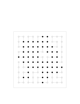
FIG. 1.: Putative compact native structure of sequence 1 from Table I ($E=-45$) according to [28]; (filled circle) H monomers, (open circle) P monomers.

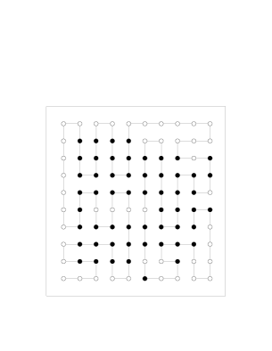
FIG. 2.: Putative compact native structure of sequence 2 from Table I ($E=-46$) according to [28].

2d HAP model

To analyze the performance of PERM on the HAP model we used $\boldmath{\epsilon}=(-4,-1,2)$ as energy parameters, for which set the inverse folding problem is solvable [25]. We choose a 3-helix structure with $N=42$, see Fig. 3, which is the ground state of the sequence $pA(HAAH)_{3}PA_{3}H_{10}A_{3}P(HAAH)_{3}Ap$, where $A$ denotes an amphipatic intra-chain group with one hydrophobic and one polar side, while $p$ denotes an amphipatic end group with one hydrophobic and two polar sides.

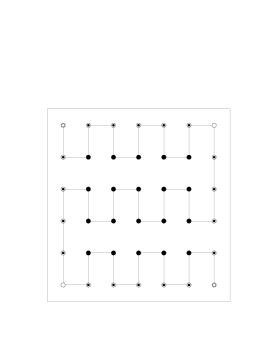
FIG. 3.: Ground state structure of the HAP sequence; (filled circle) H monomers, (structured circle) A monomers, (open circle) P monomers.

3d HP model

Ten sequences of length $N=48$ were given in [30]. Each of these sequences was designed by minimizing the energy of a particular target conformation in sequence space under the constraint of constant composition [31]. The authors tried to find the lowest energy states with two different methods, one being an heuristic stochastic approach [15], the other based on exact enumeration of low energy states [32]. With the first method they failed in all but one case to reach the lowest energy. With the second method in all but one cases they obtained conformations with energies that were even lower than the putative ground states the sequences were designed for, while for one case the ground state energy was confirmed. Precise CPU times were not quoted.

3d modified HP model

A most interesting case is a 2-species 80-mer with interactions $(-1,0,-1)$ studied first in [24]. These particular interactions were chosen instead of the HP choice $(-1,0,0)$ because it was hoped that this would lead to compact configurations. Indeed, the sequence was specially designed to form a “four helix bundle” which fits perfectly into a $4\times 4\times 5$ box, see Fig. 4. Its energy in this putative native state is $-94$. Although the authors of [24] used highly optimized codes, they were not able to recover this state by MC. Instead, they reached only $E=-91$. Supposedly, a different state with $E=-94$ was found in [28], but figure 10 of this paper, which is claimed to show this configuration, has a much higher value of $E$. Configurations with $E=-94$ but slightly different from that in [24] and with $E=-95$ were found in [29] by means of an algorithm similar to that in [28]. For each of these low energy states the author needed about one week of CPU time on a Pentium.

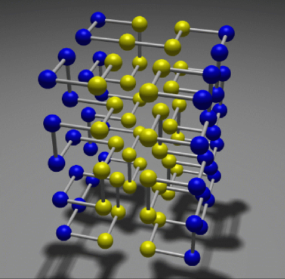
FIG. 4.: Putative native state of the “four helix bundle” sequence, see Table I, as proposed by O’Toole et al.. It has $E=-94$, fits into a rectangular box, and consists of three homogeneous layers. Structurally, it can be interpreted as four helix bundles.

3d $\infty$ monomer types

Sequences with $N=27$ and with continuous interactions were studied in [27]. Interaction strengths were sampled from Gaussians with fixed non-zero mean and fixed variance. These $N(N-1)/2$ numbers were first attributed randomly to the monomer pairs, then they were randomly permuted, using a Metropolis accept/reject strategy with a suitable cost function, to obtain good folders. Such “breeding” strategies to obtain good folders were also developed and employed by other authors for various models [31, 33, 34], and seem necessary to eliminate sequences which fold too slowly and/or unreliably. It is believed that also during biological evolution optimization processes took place with similar effects, so that actual proteins are better folders than random amino sequences.

The Algorithm

The algorithms we apply here are variants of the pruned-enriched Rosenbluth method (PERM) [17], a chain growth algorithm based on the Rosenbluth-Rosenbluth (RR) [18] method. There, monomers are placed sequentially at vacant sites either with uniform probability, or with some non-uniform probability distribution. In either case it leads to weighted samples where each configuration carries a weight $W$. For long chains or low temperatures, the spread in weights can become very wide which then leads to serious problems [35]. But since the weights accumulate as the chains grow, one can interfere during the growth process by ‘pruning’ configurations with low weights and replacing them by copies of high-weight configurations. This is in principle similar to population based methods in polymer simulations [36, 37] and in quantum Monte Carlo (MC) [38], but the implementation is different. Pruning is done stochastically: if the weight of a configuration has decreased below a threshold $W^{<}$, it is eliminated with probability 1/2, while it is kept and its weight is doubled in the other half of cases. Copying (‘enrichment’ [39]) is done independently of this. If $W$ increases above another threshold $W^{>}$, the configuration is replaced by $n$ copies, each with weight $W/n$. Technically, this is done by putting onto a stack all information needed about configurations which still have to be copied. This is most easily implemented by recursive function calls. Thereby one avoids the need for keeping large populations of configurations [36, 37, 38]. PERM has proven extremely efficient for studies of lattice homopolymers near the $\theta$ point [17]. It has also been successfully applied to phase equilibria [40], to the ordering transition in semi-stiff polymers [41], and to spiraling transitions of polymers with interactions depending on relative orientation of monomers [42]. We refer to these papers for more detailed descriptions of the basic algorithm.

The main freedom when applying PERM consists in the a priori choice of the sites where to place the next monomer, in the thresholds $W^{<}$ and $W^{>}$ for pruning and copying, and in the number of copies made each time. All these features do not affect the formal correctness of the algorithm, but they can greatly influence its efficiency. They may depend arbitrarily on chain lengths and on local configurations, and they can be changed freely at any time during the simulation. Thus the algorithm can ‘learn’ during the simulation.

In order to apply PERM to heteropolymers at very low temperatures, the strategies proposed in [17] are modified as follows.

(1) For homopolymers near the theta-point it had been found that the best choice for the placement of monomers was not according to their Boltzmann weights, but uniformly on all allowed sites [17, 40]. This might be surprising since the Boltzmann factor has then to be included into the weight of the configuration, which might lead to large fluctuations. Obviously, this effect is counterbalanced by the fact that larger Boltzmann factors correspond to higher densities and thus to smaller Rosenbluth factors [35].

For a heteropolymer this has to be modified, as there is no longer a unique relationship between density and Boltzmann factor. In a strategy of ‘anticipated importance sampling’ we should preferentially place monomers on sites with mostly attractive neighbors. Assume that we have two kinds of monomers, and we want to place a type-$A$ monomer. If an allowed site has $m_{B}$ neighbors of type $B$ ($B=H,P$), we select this site with a probability $\propto 1+a_{AH}m_{H}+a_{AP}m_{P}$. Here, $a_{AB}$ are constants with $a_{AB}>0$ for $\epsilon_{AB}<0$ and vice versa.

(2) Most naturally, $W^{>}$ and $W^{<}$ are chosen proportional to the estimated partition sum $Z_{n}$ [17]. This becomes inefficient at very low $T$ since $Z_{n}$ will be underestimated as long as no low-energy state is found. When this finally happens, $W^{>}$ is too small. Thus too many copies are made which are all correlated but cost much CPU time.

This problem can be avoided by increasing $W^{>}$ and $W^{<}$ during particularly successful ‘tours’ (a tour is the set of configurations derived by copying from a single start [17]). But then also the average number of long chains is decreased in comparison with short ones. To reduce this effect and to create a bias towards a sample which is flat in chain length, we multiply by some power of $M_{n}/M_{1}$, where $M_{n}$ is the number of generated chains of length $n$. With ${\cal N}(n)$ denoting the number of chains generated during the current tour we used therefore

$$W^{<}=C\;Z_{n}\;[(1+{\cal N}(n)/M)(M_{n}+M)/(M_{1}+M)]^{2},$$

and $W^{>}=rW^{<}$. Here, $C$ is a constant of order unity, $r\approx 10$, and $M$ is a constant of order $10^{4}-10^{5}$.

(3) Creating only one new copy at each enrichment event (as done in [17]), cannot prevent the weights from exploding at very low $T$. Thus we have to make several copies if the weight is large and surpasses $W^{>}$ substantially. A good choice for the number of new copies created when $W>W^{>}$ is int$[\sqrt{W/W^{>}}]$.

(4) Two special tricks were employed for ‘compact’ configurations of the 2-$d$ HP model filling a square. First of all, since we know in this case where the boundary should be, we added a bias for polar monomers to actually be on that boundary, by adding an additional energy of -1 per boundary site. Note that this bias has to be corrected in the weights, thus the final distributions are unaffected by it and unbiased. Secondly, in two dimensions we can immediately delete chains which cut the free domain into two disjoint parts, since they never can grow to full length. In the present simulations, we checked for this by looking ahead one time step. In spite of the additional work this was very efficient, since it reduced considerably the time spent on dead-end configurations.

(5) In some cases we did not start to grow the chain from one end but from a point in the middle. We grew first one half, and then the other. Results were averaged over all possible starting points. The idea behind this is that real proteins have folding nuclei [43], and it should be most efficient to start from such a nucleus. In some cases this trick was very successful and speeded up the ground state search substantially, in others not. We take this observation as an indication that in various sequences the end groups already provide effective nucleation sites. This is e.g. the case for the 80-mer with modified HP interactions of [24]. We also tried to grow the chain on both sides simultaneously. However it turned out that this is not effective computationally [44].

(6) In the case of the HAP model it turned out that, while the ground state configuration of the chain geometry could be reached easily, the ground state configurations of the side groups (i.e., of the H/P bond attributions of amphiphilic monomers [25]) could note be reached effectively using PERM alone. Therefore, after building the chain conformation to its full length we let the side groups of the amphipatic monomers rotate thermally using a Metropolis algorithm. This approach utilizes the short relaxation time of side group fluctuations within the subphase of a fixed chain conformation and leads to the desired ground states [45].

(7) For an effective sampling of low-lying states the choice of simulation temperature $T$ appears to be of importance. If it is too large, low-lying states will have a low statistical weight and will not be sampled reliably. On the other hand, if $T$ is too low, the algorithm becomes too greedy: configurations which look good at first sight but lead to dead ends are sampled too often, while low energy configurations, whose qualities become apparent only at late stages of the chain assembly, are sampled rarely. Of course they then get huge weights (since the algorithm is correct after all), but statistical fluctuations become huge as well. This is in complete analogy to the slow relaxation hampering more traditional (Metropolis type) simulations at low $T$ – note, however, that “relaxation” in the proper sense does not exist in the present algorithm.

In the cases we considered it turned out to be most effective to choose a temperature that is below the collapse transition temperature (note, however, that this transition is smeared out, see the results below) but somewhat above the temperature corresponding to the structural transition which leads to the native state. This observation corresponds qualitatively to the considerations of [46], although a quantitative comparison appears not to be possible.

(8) For 2-dimensional HP chains, we performed also some runs where we restricted the search for native configurations further, by disallowing non-bonded HP neighbor pairs. The idea behind this was that such a pair costs energy, and is thus less likely to appear in a native state. But this is only a weak heuristic argument. Forbidding such pairs certainly gives wrong thermal averages, and it might prevent the native state to be found, if it happens to contain such a pair. But in two cases this restriction did work, and gave states with lower energies than those we could reach without this trick.

Results

Let us now discuss our results. All CPU times quote below refer to SPARC Ultra machines with 167 MHz.

2d HP model

(a) For all chains of [13] we easily reached the ground state, except for the longest chain ($N=64$). For this chain the ground state is very regular, with all polar monomers on the outside, and with no non-bonded HP neighbors. Its energy is -42 (see fig.5). The authors of [13] were unable to recover by simulations this state and any other state with $E<-37$. Although we could not reach $E=-42$ either without special tricks, we obtained at least $E=-40$ after ca. 4h CPU time. Forbidding non-bonded HP neighbor pairs, we found the native state easily, but this cannot be really counted as a success since we knew in advance that such pairs do not appear in the native state. The difficulty posed by this sequence for PERM is obvious from fig.5: there is no folding center in this chain. No matter where one starts the assembly, one first has to construct a large part of the boundary before the interior behind this boundary is filled up. This intermediate state has a very low Boltzmann weight and acts thus as a bottleneck for PERM.

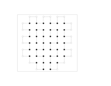
FIG. 5.: One of the ground states of the $N=64$ sequence of [13]. The other ground states differ in the configurations of the chain ends filling the interior of the structure, but have the same boundary and overall shape.

Note that the configuration of Fig.5 cannot be obtained by popular local moves including, e.g., bond exchange or crankshaft, or by reptation. But it can be reached if pivot moves are included. This illustrates that folding properties can depend strongly on the chosen kinetics.

In contrast to the sequence with $N=64$, we had no problem with the shorter sequences of [13]. In particular, for the $N=60$ sequence we found a configuration with $E=-36$ (see Table I), although the authors had quoted $E=-34$ as supposedly exact ground state energy.

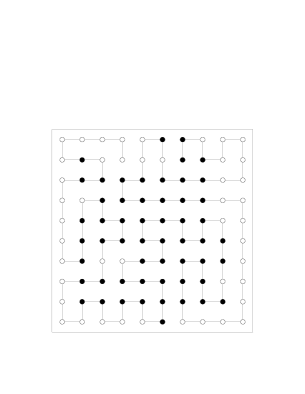
FIG. 6.: One of the compact structures of sequence 1 with energy ($E=-46$) lower than the “native” state proposed by Ramakrishnan et al..

(b) For the two HP chains of [28] with $N=100$, see Table I, we found several compact states (within ca. 40 hours of CPU time) that had energies lower than those of the compact putative ground states proposed in [28]. Figures 6 and 7 show representative compact structures with $E=-46$ for sequence 1 and $E=-47$ for sequence 2. Moreover, we found (again within 1-2 days of CPU time) several non-compact configurations with energies even lower: $E=-47$ and $E=-48$ for sequence 1 and 2, respectively. Forbidding non-bonded HP pairs, we obtained even $E=-49$ for sequence 2. Figures 8 and 9 show representative non-compact structures with these energies; a non-exhaustive collection of these is listed in

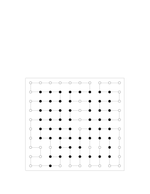
FIG. 7.: One of the compact structures of sequence 2 with lower energy ($E=-47$).

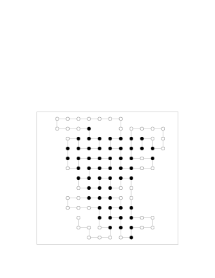
FIG. 8.: One of the (non-compact) lowest energy sequences for sequence 1 ($E=-47$).

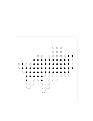
FIG. 9.: One of the (non-compact) lowest energy sequences for sequence 2 ($E=-49$).

Table I. These results reflect the well-known property that HP sequences (and those of other models) usually have ground states that are not maximally compact, see, e.g. [30], although there is a persistent prejudice to the contrary [24, 28, 47].

2d HAP model

The ground state of the HAP triple helix was found within several minutes of CPU time using the PERM-Metropolis hybrid algorithm. It was not found to be degenerate.

In order to obtain information about the folding transition, energy and contact matrix (see below) histograms were determined at $T=1.25,2$, and 4. Free energy differences, necessary for combining the histograms [48], were determined using Bennet’s acceptance ratio method [49].

FIG. 10.: Number of native contacts, total number of contacts, and energy $E$ $vs$ temperature $T$ for the HAP sequence of Fig. 3.

In Fig. 10 the thermal behavior of the mean number of contacts, number of native contacts, and of the mean energy is shown. While the structural transition to the ground state phase is best monitored by the number of native contacts and takes place around $T=1$, the compactification of the polymer chain is most clearly seen in the mean number of all contacts and in the radius of gyration (not shown here). It takes place already at much higher temperatures and is smeared out over a wide temperature range. Note that the number of all contacts follows closely the behavior of the energy.

These two transitions are seen more clearly when the fluctuations of the above order parameters are considered, see Fig. 11. Energy and contact number fluctuations exhibit a broad maximum around $T=3.5$, while the structural transition is indicated by a narrow peak of the fluctuations of the number of native contacts and of the specific heat near $T=1.0$. Note that specific heat and energy fluctuations emphasize the two transitions differently due to the factor $T^{2}$ by which they differ.

FIG. 11.: Fluctuations of the number of native contacts, total number of contacts, and energy $E$ $vs$ temperature $T$ for the HAP sequence of Fig. 3; Since energy fluctuations and specific heat emphasize the polymer collapse and structural transition differently, we have included the specific heat, too.

3d HP model

With PERM we succeeded to reach ground states of the ten sequences of length $N=48$ given in [30] in all cases, in CPU times between a few seconds and 5 hours, see Table II. In these simulations we used a rather simple version of PERM, where we started assembly always from the same end of the chain. We found that the sequences most difficult to fold were also those which had resisted previous Monte Carlo attempts [30]. In those cases where a ground state was hit more than once, we verified also that the ground states were highly degenerate. In no case there were gaps between ground and first excited states, see Fig. 12. Therefore, none of these sequences is a good folder, though they were designed specifically for this purpose.

3d modified HP model

For the two-species 80-mer with interactions $(-1,0,-1)$, even without much tuning our algorithm gave $E=-94$ after a few hours, but it did not stop there. After a number of rather disordered configurations with successively lower energies, the final candidate for the native state has $E=-98$. It again has a highly symmetric shape, although it does not fit into a $4\times 4\times 5$ box, see Fig. 13. It has twofold degeneracy (the central $2\times 2\times 2$ box in the front of Fig. 13 can be flipped), and both configurations were actually found in the simulations. Optimal parameters for the ground state search in this model are $\beta=1/kT\approx 2.0$, $a_{PP}=a_{HH}\approx 2$,

TABLE II.: PERM performance for the binary sequences from [30].

sequence	$-E_{\rm min}$a	$-E_{\rm MC}$b	$n_{\rm success}$c	CPU time
nr.				(min)
1	32	31	101	6.9
2	34	32	16	40.5
3	34	31	5	100.2
4	33	30	5	284.0
5	32	30	19	74.7
6	32	30	24	59.2
7	32	31	16	144.7
8	31	31	11	26.6
9	34	31	1	1420.0
10	33	33	16	18.3

FIG. 12.: Energy spectrum of the ten sequences given in [30]. More precisely, to emphasize the low-energy part of the spectrum, we show the histograms obtained from the spectra by multiplying with $e^{E/T},\;T=0.334$. Note that there are no energy gaps in any of these spectra.

and $a_{HP}\approx-0.13$. With these, average times for finding $E=-94$ and $E=-98$ in new tours are ca. 20 min and 80 hours, respectively.

A surprising result is that the monomers are arranged in four homogeneous layers in Fig. 13, while they had formed only three layers in the putative ground state of Fig. 4. Since the interaction should favor the segregation of different type monomers, one might have guessed that a configuration with a smaller number of layers should be favored. We see that this is outweighed by the fact that both monomer types can form large double layers in the new configuration. Again, our new ground state is not ‘compact’ in the sense of minimizing the surface, and hence it also disagrees with the wide spread prejudice that native states are compact.

In terms of secondary structure, the new ground state is fundamentally different from the putative ground state

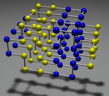
FIG. 13.: Conformation of the “four helix bundle” sequence with $E=-98$. We propose that this is the actual ground state. Its shape is highly symmetric although it does not fit into a rectangular box. It is not degenerate except for a flipping of the central front $2\times 2\times 2$ box.

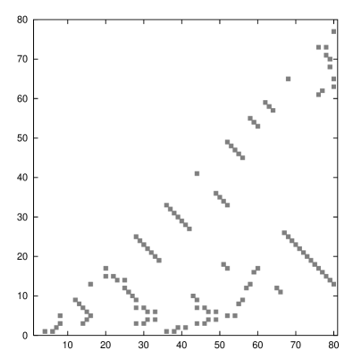
FIG. 14.: Contact matrix of the structure in Fig. 13; a black point at $(i,j)$ indicates that there is a contact between monomer $i$ and monomer $j$; grey points indicate contacts in only one of the two native states, corresponding to the twofold degeneracy of the central $2\times 2\times 2$ box. Note that the lines orthogonal to the main diagonal correspond to anti-parallel $\beta$ sheet secondary structure elements, see e.g. [50].

FIG. 15.: For comparison, the contact matrix of the putative ground state of Ref. [28] in Fig. 4; note that point triples close to the diagonal parallel as well as orthogonal to it are signatures of 3d helical secondary structure elements, see e.g. [50]; the other points denote tertiary contacts between helices.

FIG. 16.: Histograms of (top) thermal weight, (middle) radius of gyration, $R^{2}_{G}$, and (bottom) end-to-end distance, $R^{2}_{ee}$, $vs$ energy $E$ for the 80-mer “four helix bundle” at $T=0.75$.

FIG. 17.: (top) Average end-to-end distance, $R^{2}_{ee}$, and radius of gyration, $R_{G}^{2}$, (middle) specific heat per monomer, $C_{v}$, and average energy per monomer, $<E>$, $vs$ temperature $T$ for the 80-mer “four helix bundle”.

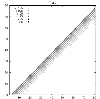
FIG. 18.: Thermally averaged contact matrix for the 80-mer “four helix bundle” in the random coil phase ($T=2.0$). Different shades of grey denote different probabilities for the contact to exist.

of Ref. [28]. While the new structure (Fig. 13) is dominated by $\beta$ sheets, which can most clearly be seen in the contact matrix (see Fig. 14), the structure in Fig. 4 is dominated by helices, see also the corresponding contact matrix in Fig. 15.

FIG. 19.: Thermally averaged contact matrix for the 80-mer “four helix bundle” in the collapsed but unstructured phase ($T=0.85$).

In order to analyze the folding transition of this sequence we again constructed histograms of the distribution of energy, end to end distance, and radius of gyration, by combining the results obtained at various temperatures between $T=0.45$ and 3. Figure 16 shows these distributions, reweighted so that it corresponds to $T=0.75$. The thermal behavior of these order parameters as functions of $T$ is obtained by Laplace transform, and is shown in Fig. 17. The behavior of energy, end-to-end distance and radius of gyration follow closely each other and exhibit clearly only the smeared out collapse of the chain from a random coil to some unstructured compact phase. In contrast, the specific heat exhibits more structure: the shoulder around $T=1$ corresponds again to the coil-globule collapse, but there are additional transitions seen around $T=0.62$ and $T=0.45$. The last one is the transition to the $\beta$-sheet dominated native phase. However, the transition at $T=0.62$ is from a unstructured globule to an intermediate phase that is helix-dominated but exhibits strong tertiary fluctuations. These structural transitions are illustrated in Figs 18 to 22 where the thermally averaged contact matrices are shown for the respective phases.

The intermediate, helix-dominated phase is particularly interesting. To it apply some of the usual characteristics of a molten globule state [51]: i) compactness, ii) large secondary structure content (although not necessarily native), and iii) strong fluctuations. This qualifies it as a candidate for a molten globule state, a phase that is absent in the folding transition of the HAP sequence [52].

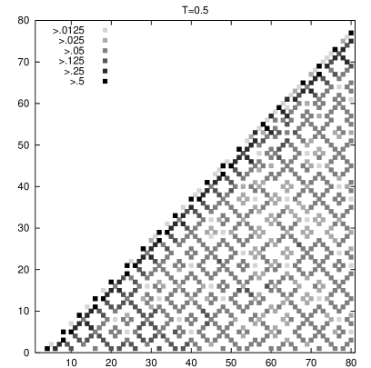
FIG. 20.: Thermally averaged contact matrix for the 80-mer “four helix bundle” in the intermediate helix-dominated phase ($T=0.5$).

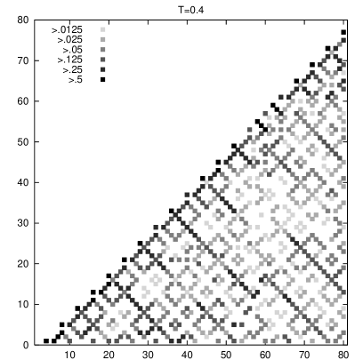
FIG. 21.: Thermally averaged contact matrix for the 80-mer “four helix bundle” at the transition from the intermediate helix-dominated phase to the $\beta$-sheet dominated phase ($T=0.4$).

3d $\infty$ monomer types

For all sequences with $N=27$ from [27] we could reach the supposed ground state energies within $<1$ hour. In no case we found energies lower than those quoted in [27], and we verified also the energies of low-lying excited states given in [27]. Notice that these sequences were designed to be good folders by the authors of [27].

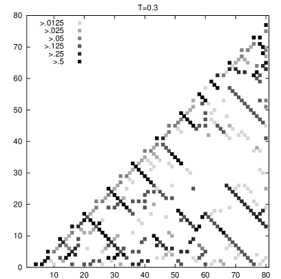
FIG. 22.: Thermally averaged contact matrix for the 80-mer “four helix bundle” in the $\beta$-sheet dominated phase ($T=0.3$).

This time the design had obviously been successful, which is mainly due to the fact that the number of different monomer types is large. All sequences showed some gaps between the ground state and the bulk of low-lying states, although these gaps are not very pronounced in some cases.

More conspicuous than these gaps was another feature: all low lying excited states were very similar to the ground state, as measured by the fraction of contacts which existed also in the native configuration. Stated differently, if the gaps were not immediately obvious, this was because they were filled by configurations which were very similar to the ground state and can therefore easily transform into the native state and back. Such states therefore cannot prevent a sequence from being a good folder. For none of the sequences of [27] we found truely misfolded low-lying states with small overlap with the ground state.

Figure 23 illustrates this feature for one particular sequence. There we show the overlap $Q$, defined as the fraction by non-bonded nearest-neighbor ground state contacts which exist also in the excited state, against the excitation energy. For this and for each of the following figures, the 500 lowest-lying states were determined. We see no low energy state with a small value of $Q$. To demonstrate that this is due to design, and is not a property of random sequences with the same potential distribution, we show in Fig. 24 the analogous distribution for a random sequence.

FIG. 23.: Overlap with ground state, $Q$, $vs$ energy $E$ of the lowest energy conformations for sequence no. 70 of Ref. [27].

FIG. 24.: Overlap with ground state, $Q$, $vs$ energy $E$ of the lowest energy conformations for a single random sequence.

To demonstrate that this difference is not merely due to a statistical fluctuation, we show in Fig. 25 the distributions for ten sequences from [27] collected in a single plot. Since the ground state energies differ considerably for different sequences, we used normalized excitation energies $(E-E_{0})/E_{0}$ on the x-axis. Analogous results for ten random sequences are shown in Fig. 26. While there is no obvious correlation between $Q$ and excitation energies for the random case, all low energy states with small $Q$ have been eliminated in the designed sequences (note the different ranges of $Q$ in Figs. 25 and 26).

This elimination of truely misfolded low energy states without elimination of native-like low energy states might be an unphysical property of the design procedure used in [27], but we do not believe that this is the case. Rather,

FIG. 25.: Overlap with ground state, $Q$, $vs$ energy $E$ of the lowest energy conformations for sequences no. 61 to 70 of Ref. [27]; for better visibility, the same symbol is used for all sequences.

FIG. 26.: Overlap with ground state, $Q$, $vs$ energy of the lowest energy conformations for ten random sequences; for better visibility, the same symbol is used for all sequences.

it should be a general feature of any design procedure, including the one due to biological evolution. It contradicts the claim of [26] that it is only the gap between native and first excited state which determines foldicity. On the other hand, our results are consistent with the “funnel” scenario for the protein folding process [53], where the folding pathway consists of states successively lower in energy and closer to the native state.

We note that for random sequences there are also excited states that have unit overlap with the native state, a feature not present in the folding sequences. These are cases where the native state has open loops and/or dangling ends, so that more compact conformations have all contacts of the native state, but have – in addition – energetically unfavorable contacts resulting in a higher total energy.

Summary and Outlook

We showed that the pruned-enriched Rosenbluth method (PERM) can be very effectively applied to protein structure prediction in simple lattice models. It is suited for calculating statistical properties and is very successful in finding native states. In all cases it did better than any previous MC method, and in several cases it found lower energy states than those which had previously been conjectured to be native.

We verified that ground states of the HP model are highly degenerate and have no gap, leading to bad folders. For sequences that are good folders we have established a funnel structure in state space: low-lying excited states of well-folding sequences have strong similarities to the ground state, while this is not true for non-folders with otherwise similar properties.

Especially, we have presented a new candidate for the native configuration of a “four helix bundle” sequence which had been studied before by several authors. The ground state structure of the “four helix bundle” sequence, being actually $beta$-sheet dominated, differs strongly from the helix-dominated intermediate phase. This sequence, therefore, should not be a good folder.

Although we have considered only lattice models in this paper, we should stress that this is not an inherent limitation of PERM. Straightforward extensions to off-lattice systems are possible and are efficient for homopolymers at relatively high temperatures [17]. Preliminary attempts to study off-lattice heteropolymers at low $T$ have not yet been particularly successful, but the inherent flexibility of PERM suggests several modifications which have not yet been investigated in detail. One of them are hybrid PERM-Metropolis approaches similar to that used for the HAP model in the present paper. Its success also suggests that similar hybrid approaches should be useful for models with more complicated monomers. Another improvement of PERM which could be particularly useful for off-lattice simulations might consist in more sophisticated algorithms for positioning the monomers when assembling the chain. Work along these lines is in progress, and we hope to report on it soon.

- [1] L. M. Gierasch and J. King (eds.), Protein Folding, Deciphering the Second Half of the Genetic Code (AAAS, New York, 1990)
- [2] T.E. Creighton (ed.), Protein Folding (Freeman, New York, 1992)
- [3] K. M. Merz Jr. and S. M. LeGrand (eds.), The Protein Folding Problem and Tertiary Structure Prediction (Birkhäuser, Boston, 1994)
- [4] H. Bohr and S. Brunak(eds.), Protein Folds: A Distance Based Approach (CRC Press, Boca-Raton/FL. 1996).
- [5] K. E. Drexler, Engines of Creation, (Anchor Books, 1986); available also on the web at the URL http://www.asiapac.com/EnginesOfCreation/.
- [6] M. Groß, Expeditionen in den Nanokosmos, (Birkhäuser, Basel, 1995).
- [7] G. M. Crippen and V. N. Maiorov, in [3], p.231-277.
- [8] A. Kolinski and J. Skolnick, Lattice Models of Protein Folding, Dynamics and Thermodynamics, (Chapman & Hall, New York, 1996).
- [9] L. A. Mirny and E. I. Shakhnovich, J. Mol. Biol. 264 1164 (1996).
- [10] A. Sali, E. I. Shakhnovich and M. Karplus J. Mol. Biol. 235 1614 (1994).
- [11] U. H. E. Hansmann and Y. Okamoto, J. Comp. Chem. 14, 1333 (1993); Physica A 212, 415 (1994); Phys. Rev. E 54, 5863 (1996).
- [12] S. R. Wilson and W. Cui, in [3], p.43-70.
- [13] R. Unger and J. Moult, J. Mol. Biol. 231, 75 (1993)
- [14] S. M. LeGrand and K. M. Merz jr., in [3], p.109-124.
- [15] K. A. Dill, K. M. Fiebig and H. S. Chan, Proc. Natl. Acad. Sci USA 90, 1942 (1993).
- [16] F. Eisenhaber, B. Persson and P. Argos, Crit. Rev. Biochem. Mol. Biol. 30, 1 (1995).
- [17] P. Grassberger, Phys. Rev. E, in press (1997)
- [18] M.N. Rosenbluth and A.W. Rosenbluth, J. Chem. Phys. 23, 256 (1955)
- [19] H. Frauenkron, U. Bastolla, E. Gerstner, P. Grassberger and W. Nadler, submitted (1997).
- [20] Y. Kantor and M. Kardar, Europhys. Lett. 28, 169 (1994)
- [21] K.A. Dill, Biochemistry 24, 1501 (1985)
- [22] K.F. Lau and K.A. Dill, Macromolecules 22, 3986 (1989); J. Chem. Phys. 95, 3775 (1991); H.S. Chan, and K.A. Dill, J. Chem. Phys. 95, 3775 (1991)
- [23] N.D. Socci and J.N. Onuchic, J. Chem. Phys. 101, 1519 (1994)
- [24] E. O’Toole and A. Panagiotopoulos, J. Chem. Phys. 97, 8644 (1992)
- [25] T. Krausche and W. Nadler, to be published (1997).
- [26] A. Sali, E. I. Shakhnovich and M. Karplus, Nature 369 248 (1994).
- [27] D.K. Klimov and D. Thirumalai, PROTEINS: Structure, Function and Genetics 26, 411 (1996); sequences are available from http://www.glue.umd.edu/klimov.
- [28] R. Ramakrishnan, B. Ramachandran and J.F. Pekney, J. Chem. Phys. 106, 2418 (1997)
- [29] J.M. Deutsch, J. Chem. Phys. 106, 8849 (1997).
- [30] K. Yue et al., Proc. Natl. Acad. Sci. USA 92, 325 (1995)
- [31] E. I. Shakhnovich and A. M. Gutin, Proc. Natl. Acad. Sci USA 90, 7195 (1993); E. I. Shakhnovich, Phys. Rev. Lett. 72, 3907 (1994).
- [32] K. Yue and K. A. Dill, Proc. Natl. Acad. Sci USA 92, 146 (1995).
- [33] M. Ebeling and W. Nadler, Proc. Natl. Acad. Sci. USA 92, 8798 (1995); Biopolymers 41, 165 (1997).
- [34] J.M. Deutsch and T. Kurosky, Phys. Rev. Lett. 76, 323 (1996).
- [35] J. Batoulis and K. Kremer, J. Phys. A 21, 127 (1988)
- [36] T. Garel and H. Orland, J. Phys. A 23, L621 (1990)
- [37] B. Velikson, T. Garel, J.-C. Niel, H. Orland and J.C. Smith, J. Comput. Chem. 13, 1216 (1992)
- [38] C.J. Umrigar, M.P. Nightingale, and K.J. Runge, J. Chem. Phys. 99, 2865 (1993)
- [39] F.T. Wall and J.J. Erpenbeck, J. Chem. Phys. 30, 634, 637 (1959)
- [40] H. Frauenkron and P. Grassberger, preprint cond-mat/9707101 (1997)
- [41] U. Bastolla and P.Grassberger, preprint cond-mat/9705178 (1997)
- [42] G. T. Barkema, U. Bastolla, and P. Grassberger, preprint cond-mat/9707312 (1997)
- [43] R. R. Matheson and H. A. Scheraga, Macromolecules 11, 819 (1978).
- [44] At first sight, one might believe that allowing the chain to grow at both ends should decrease the attrition rate and hence be advantageous. For homopolymers one can see easily that this is not true. Attrition is actually decreased, since chains which have one end blocked can still grow at the other end. But such chains have small Rosenbluth factors and thus extremely low in average. Therefore, they just cost efforts without efficiently contributing to statistical averages. For heteropolymers this argument no longer holds, however, and it is not clear why growing the chain at both ends is not efficient either.
- [45] Note, however, that there exists an alternative approach: for a fixed chain geometry a computationally effective ( instead of ) complete enumeration of all side group conformations is possible; E. Gerstner, P. Grassberger and W. Nadler, to be published.
- [46] A. V. Finkelstein, A. M. Gutin and A. Y. Badretdinov PROTEINS: Structure, Function and Genetics 23, 151 (1995).
- [47] E. I. Shakhnovich and A. M. Gutin, J. Chem. Phys. 93 5967 (1990); A. M. Gutin and E. I. Shakhnovich, J. Chem. Phys. 98 8174 (1993).
- [48] A.M. Ferrenberg and R.H. Swendsen, Phys. Rev. Lett. 61, 2635 (1988); 63, 1195 (1989)
- [49] C. H. Bennet, J. Comp. Phys. 22, 245 (1976).
- [50] H. S. Chan and K. A. Dill, Macromolecules 22 4559 (1989); J. Chem. Phys. 92, 3118 (1990).
- [51] H. Christensen and R. H.Pain, Europ. Biophys. J. 19, 221 (1991).
- [52] In [29], indications for the -sheet phase were found, too, and on this basis an analogy to the competition of structures in the prion problem [see, e.g., J. Nguyen et al., Biochemistry 34, 4186 (1995)] was drawn. However, our results showing that the helical phase is strongly structurally disordered demonstrate that this analogy cannot be perfect. In a model for prions, both competing phases should be much more well defined.
- [53] P. G. Wolynes, J. N. Onuchic, and D. Thirumalai, Science 267, 1619 1995).