Traveling through potential energy landscapes of disordered materials: the activation-relaxation technique

Abstract

A detailed description of the activation-relaxation technique (ART) is presented. This method defines events in the configurational energy landscape of disordered materials such as a-Si, glasses and polymers, in a two-step process: first, a configuration is activated from a local minimum to a nearby saddle-point; next, the configuration is relaxed to a new minimum; this allows for jumps over energy barriers much higher than what can be reached with standard techniques. Such events can serve as basic steps in equilibrium and kinetic Monte Carlo schemes.

]

I Introduction

Microscropic structural phenomena often proceed on time scales remarkably long compared to those of the atomistic oscillations. This is the case, for example, for glassy materials where microscopic dynamics takes place over time scales orders of magnitude larger than that associated with the natural atomistic time scale, set by the phonon frequency of typically $10^{13}Hz$. Such a discrepancy is best understood from the configurational energy landscape: the system finds itself in a deep minimum surrounded by energy barriers which are many times larger than its temperature. Only rare fluctuations of thermal energies will allow the system to jump over a barrier and move to a new minimum. Typically, the rate for such jumps decreases exponentially with increasing barrier height, and may reach macroscopic values — of the order of seconds or more, rendering the study of these phenomena rather difficult.

These long time scales are especially prohibitive for numerical studies. Traditional methods for the study of structural relaxation are of two kinds: molecular dynamics (MD) and Monte-Carlo (MC). MD is based on the direct integration of the equations of motion. In order to ensure the stability of the solution, the integration step cannot be larger than a fraction of a typical phonon vibration, i.e., somewhere between 1 and 10 fs. Depending on the number of atoms, the interaction potential, and the speed of the computer, the total number of steps can reach $10^{4}$ to $10^{7}$, which translates into a time-scale on the order of nanoseconds; this is still far from the experimental time-scale for structural relaxation of glassy materials. Because of the nature of MD, improvements beyond the linear level are particularly difficult to achieve. Recently, a promising scheme involving a mixture of transition-state theory and MD has achieved a significant speed-up in the simulation of a model system [3]; it is however too early to say how successful this scheme will be for generic problems.

The inherent limitation to the degree of structural relaxation achieved with MD does not apply a priori to MC schemes. Here, the speed of structural relaxation is mostly determined by the nature of the attempted moves. Until now, most algorithms have used moves defined in real space, involving the displacement of either one or a limited number of atoms. Single-atom moves are rather efficient in liquids [4]; however, they are not as successful in reproducing the collective nature of structural relaxation associated with the slow dynamics of glassy and amorphous materials. Algorithms with more complex moves exist: the bond-switching algorithm of Wooten, Winer and Weaire,[5] for instance, succeeds in producing some of the best continuous random network models of amorphous semiconductors. Such algorithms are however problem-specific, and their dynamics generally unphysical.

In lattice models like the Ising model, it is often possible to move from microscopic events — single spin-flips in the traditional Metropolis and heat-bath Monte-Carlo simulations – to collective events determining the behavior over longer times — flips of clusters of spins. Doing so can lead to a substantial improvement in the speed of algorithms, especially near the critical temperature where the correlation length and thus the cluster size diverges. The cluster algorithm of Swendsen and Wang [6] for example, can increase the computational performance of the simulation by many orders of magnitude compared to single-spin flip algorithms.

In this paper, we give a detailed description of a recently proposed method which introduces a similar change of paradigm for continuum-based models: from the microscopic single-atom displacements to collective moves which form the basis of the activated processes in glassy and amorphous materials. This method, the activation-relaxation technique (ART), has already been applied with success to amorphous semiconductors and metallic glasses[7, 8, 9]. With a similar algorithm, Doye and Wales have studied the potential energy surface of small Lennard-Jones clusters[10].

An event in ART is defined as a move from a local energy minimum $\vec{M}^{(0)}\equiv(\vec{x}^{(0)}_{1},\dots,\vec{x}_{N}^{(0)})$ to another nearby minimum $\vec{M}^{(1)}\equiv(\vec{x}_{1}^{(1)},\dots,\vec{x}_{N}^{(1)})$ following a two-step process mimicking a physical activated processes:

  i)

the activation during which a configuration is pushed from a local minimum to a nearby saddle-point;

  ii)

the relaxation which brings the configuration from this saddle-point to a new local minimum.

By defining the moves in the $3N$-dimensional space controlling the dynamics of relaxation – the configurational energy landscape – ART removes any constraint on the type of real space moves allowed. This is particularly important in disordered and complex materials where events can involve very complex local or collective rearrangements that are hard to foresee.

This paper is organized as follows: we first present the activation–relaxation technique. The following section discusses the implementation of the algorithm. We finally show examples of events in amorphous silicon (a-Si) and silica glas (g-SiO₂).

II The activation–relaxation technique

In many materials and systems, the dynamics can be accurately described as a sequence of metastables states separated by energy barriers high compared to $k_{B}T$, the typical energy scale at the atomic level. Such metastable configurations will remain essentially unchanged on a time long compared with the natural time-scale set by lattice vibrations, and can be well identified by the atomic positions at zero K, i.e., by the local minimum of the configurational energy landscape. Knowledge of the distribution and properties of these local minima is sufficient for determining the thermodynamical properties of the system. To understand the dynamical properties of these materials, however, a knowledge of the rates controlling the jumps from one minimum to another is also necessary.

To a first approximation, the dynamics in these materials is determined by the activation energy, i.e. the energy needed to bring a configuration from the local minimum to a nearby saddle-point. Because of the exponential nature governing the energy fluctuations, any event following another trajectory, with by definition an energy higher than that at the saddle-point, will be much less probable and can be safely neglected. [11] For the simplest characterization of the non-equilibrium properties or dynamics of a disorder material away from the glass transition it is therefore sufficient to map the continuous configurational energy landscape onto a network formed by minima connected via trajectories going through first-order saddle-points.[12] The current ART method provides a local prescription for exploring this simplified space through hops from a local minimum to another (events).

By defining the events directly in the configurational energy landscape, which, as we have seen, fully determines the dynamical and equilibrium properties of a material, ART becomes much less sensitive to the details of the real space configuration. Doing so, it refrains from defining a priori the type of atomic rearrangements leading to structural relaxation. In effect, it is the system itself which determines the appropriate atomic processes, in much closer agreement with real processes. Such a change in paradigm, from real to configurational space, is particularly necessary for the study of glassy materials where an unambiguous description of real-space configurations in terms of neighbor lists, coordination defects, etc./ is generally impossible to give. ART is a priori blind to the details of real space configurations; all ART needs is a local and continuous description of an energy-landscape; discontinuous energy landscapes, as, for instance, in discrete spin models, cannot be differentiated and thus forces are not defined. Any continuous interaction potential however, from Lennard-Jones to LDA, can in principle be used with ART.

As mentioned in the introduction, the activation-relaxation technique consists of two parts: a path from a local energy minimum to a nearby saddle-point — the activation; and a trajectory from this point to a new minimum — the relaxation.

The relaxation to an energy minimum poses no particular challenge: it is a well-defined and well-behaved operation for which a number of efficient algorithms are available (see, for example, Ref. [13]).

The activation from a minimum to a saddle-point requires more care: to our knowledge, no theoretical framework exists that allows for finding the complete set of saddle-points around a local minimum. A number of works have been devoted to the study of finding the transition states in clusters and low-dimensional systems. Many of the techniques, however, start with the knowledge of both minimum states and try to find the path connecting the two.[14] It is a very different problem to try to find a saddle-point with the knowledge of only one minimum. Most methods can be traced back to two techniques, the distinguished coordinate [15, 16] and the eigenvector-following[10, 17, 18] algorithms. Although these methods are generic, neither addresses the question of the generation of a complete set of saddle-points around a given minimum.

In steepest-descent — or zero-temperature Langevin dynamics where the velocity is proportional to the force — all trajectories, including those starting at a saddle-point, lead to a local energy minimum. A naive approach to find the trajectory from a minimum to a nearby saddle-point would therefore be to retrace this path using a time-reversed zero-temperature Langevin dynamics, or steepest-ascent algorithm. This fails, however, since using steepest-ascent simply corresponds to inverting the sign of the total energy, in effect exchanging local minima with local maxima. Moreover, the minimum-energy trajectory leading from a local minimum to a saddle-point is an unstable trajectory for steepest-ascent; any perturbation sends the path away from the reversed steepest-descent trajectory.

Within Newtonian mechanics a trajectory from a saddle-point to a minimum is also time-reversible: starting at a minimum with properly chosen velocities, one would be able to move up to any saddle-point. In contrast to time-reversed Langevin dynamics, the trajectory cannot reach divergent parts of the configurational energy landscape since the total energy is conserved. As with time-reversed zero-temperature Langevin dynamics, though, even a very tiny deviation can bring the system far away from the saddle-point. Sampling a very large number of initial random displacements and then targeting the least divergent trajectories, Dykman et al. could successfully find the saddle-points of a chaotic two-dimensional system.[19] If this approach can work for a simple energy function in low dimensions, such a hit-and-miss algorithm becomes hopeless in a large 3N-dimensional space with a computationally expensive force to evaluate.

At the saddle-point, all eigenvalues of the Hessian but one are positive. The energy landscape resembles a valley going down along the eigen directions corresponding to the negative eigenvalue. Leaving the saddle-point by steepest-descent we follow the floor of the valley to eventually arrive at a nearby minimum. This suggests immediately a local algorithm which should be more stable than the steepest-ascent: to define a trajectory to a saddle-point, the configuration is moved in such a way as to minimize the force along all directions but the one corresponding to the lowest eigenvalue. This eigenvalue is identified with the local bottom of the valley, and the configuration is moved against the force along this direction. A small displacement away from the bottom of the valley would be corrected for by the $(3N-1)$-dimensional minimization, making the trajectory stable. Intuitively, this line and the path of steepest-descent should run mostly parallel; they are not identical though, and sometimes diverge.

In most circumstances, this algorithm will converge to a saddle-point. Because we consider here the maximization along a single eigendirection, this algorithm will not lead to second- or higher-order saddle-points. This is in essence what was proposed by Cerjan and Miller for the location of transition states in low-dimensional energy surfaces[17], and what was used for an extensive study of a 13-atom LJ cluster by Doye and Wales[10].

Because of its $N^{3}$ requirements, this algorithm becomes rapidly too computer intensive for realistic bulk systems, often demanding many hundreds of atoms with a costly energy function. We must therefore find another algorithm which does not require evaluation of the full Hessian matrix at each step.

The current implementation of ART follows a modified force vector $\vec{G}$, obtained by inverting the component of the force parallel to the displacement from the current position to the local minimum $\vec{r}=\vec{X}-\vec{M}^{(0)}$ while minimizing all other $3N-1$ directions:

$$\vec{G}=\vec{F}-(1+\alpha)(\vec{F}\cdot\hat{r})\hat{r}$$ (1)

where $\hat{r}$ is the normalized vector parallel to $\vec{r}$, $\vec{F}$ is the total force on the configuration as calculated using an interaction potential, and $\alpha$ is a control parameter. This equation is applied iteratively until the force parallel to the displacement from the minimum $\vec{F}\cdot\hat{r}$ changes sign from negative to positive. Generally, the force perpendicular to the displacement decreases rapidly after a few iterations, bringing the configuration close to the steepest-ascent trajectory. For a steepest-ascent path perfectly parallel to $\vec{r}$, the modified force of Eq. (1) strictly sticks to the floor of the valley up to the saddle-point; for steepest-ascent trajectories perpendicular to $\vec{r}$, the algorithm fails. From experience, such trajectories are rare and the algorithm generally converges to a saddle-point.

Since moves are defined in the configurational energy landscape, vectors in Eq. (1) have $3N$ components both for the force and the position;[20] the displacement of the configuration from a local minimum to a nearby saddle-point may therefore involve any number of atoms — from one to all $N$ atoms.

In disordered networks, it is unlikely that the lowest eigenvalue of the Hessian matrix is degenerate. There are therefore always only two valleys stemming out of the local minimum, corresponding to the positive and negative direction of the lowest eigenvector. Thus, following valleys from the minimum either along the lowest eigenvector or the modified force leads to only two saddle-points, whereas a system typically has many, even thousands of saddle-points. Even worse, these two directions correspond, in bulk materials, to long-wavelength distorsions and do not lead to interesting events. Finding a way to avoid these directions can be a difficult task.

One approach, taken by Doye and Wales for the study of a 13-atom Lennard-Jones cluster, is to select in turn each of the eigendirections of the Hessian at the minimum and follow it to a nearby saddle-point.[10] Since there are only 78 such directions, only a fraction of the many ($\approx 10^{3}$, see Ref. [21]) saddle-points can be reached this way from the minimum; local information around the minimum is insufficient to locate all valleys leading to saddle-points. Moreover, the repeated calculation of the Hessian is an expensive operation for large systems.

We propose a few approaches that do not require $O(N^{3})$ operations and work for a wide spectrum of circumstances; these are discussed in section III.

Once a valley has been found, the situation becomes more straightforward, and we can use either of the algorithms described above to follow the valley to the saddle-point.

III The implementation

The implementation of the method poses no particular conceptual or computational problems. The whole code, except for the force and total energy calculation, contains a few hundred lines at most. Its core consists of three parts: the escape from the harmonic basin, the convergence to the saddle-point, and the relaxation to a minimum.

A Escaping the harmonic basin

The part of the algorithm that is most sensitive to details of the system studied is the escape from the harmonic basin; different approaches might have to be tried to find the most effective one. In general, open but stiff materials like amorphous semiconductors have a very small harmonic basin from which it is easy to escape. More compact materials — metallic glasses — or floppier ones — silica glasses — pose more problems. To ensure a proper sampling of events, any method for escaping the harmonic basin that leaves out a significant fraction of the saddle-points should be avoided.

The simplest way of escaping a harmonic basin is to make a random displacement away from the minimum, involving a single randomly chosen atom, a cluster, or all atoms. In our experience, for small systems they all lead to the same type of events; for larger systems, a global random displacement tends to induce many spatially separated events which become difficult to disentangle. We therefore prefer a local displacement for systems of more than a few hundred atoms.

A random direction generally has a sizable overlap with the softest elastic modes, and tends to fall back to these easily. We get better results by taking the escape direction for the initial displacement along the force induced by a small random displacement; this procedure is essentially equivalent to applying the Hessian matrix to a random vector, resulting in a first–order suppression of the softest elastic modes.

For small systems, where the Hessian can be obtained and diagonalized in a relatively short time, the softest modes can be removed directly from a random initial direction, or the initial displacement can be chosen along a linear combination of the stiffest eigendirections. This approach is rather computationally involved and cannot be reasonably carried out for systems with more than 100 or 200 atoms.

Once the initial direction is fixed, it is then followed until the passage of some threshold, indicating that the harmonic region has been left. This threshold has to be large enough to ensure that the trajectory does not fold back onto the softest direction while remaining insde the basin of attraction. We use a combination of two conditions for determining the point where the configuration has left the harmonic region surrounding the initial minimum: when the force component parallel to the displacement either stops increasing or when the ratio of this component to the perpendicular component is smaller then a given fraction, we consider the harmonic region left and the ART procedure as such begins.

In the algorithm used in Refs. [7], [8] and [9], no clear distinction was made between leaving the harmonic region and convergence to the saddle-point; instead, an additional repulsive harmonic potential was introduced, which is added around the minimum with a strength $A_{rep}$ and a range $r_{c}$:

$$E_{rep}=A_{rep}(|\vec{r}|-r_{c})^{2}.$$ (2)

Although relatively efficient, this approach modifies the local energy landscape and introduces an artificial length scale $r_{c}$ in the problem. To reduce the impact of this additional length scale, one can re-initialize $r_{c}$ and $A_{rep}$ at random before each event.

Currently we prefer to take as initial direction the force after a random displacement, and follow that direction until we leave the harmonic region, and then follow $\vec{G}$ as defined in Eq. (1) until the saddle-point is reached.

B Convergence to a saddle-point

Convergence to the saddle-point cannot be achieved using standard minimization techniques because the modified force $\vec{G}$ as defined in Eq. (1) is not curl-free, i.e., it cannot be obtained from the gradient of a scalar. We therefore have to follow closely the direction of $\vec{G}$ until we reach the saddle-point, indicated by a change of sign in the component of the force parallel to $\vec{r}$. Many simple algorithms can readily be adapted for this purpose. Making small displacements in the direction of $\vec{G}$ is the most obvious choice for reaching a saddle-point. Such a crude method, however, is rather unstable and can easily enter into oscillations or severe slowing down.

The conjugate-gradient (CG) algorithm provides an easy solution to this restriction by ensuring that the new displacement will be in a direction conjugate to the previous ones.[13] The line minimization along a direction $\hat{h}$ required in the CG implementations of numerical packages, however, are based on the existence of a total energy - which cannot be defined. We replace it by a root-finding algorithm of $\vec{G}\cdot\hat{h}$. In general, only a couple of force evaluations are necessary to reach that point.

The Levenberg-Marquardt (LM) algorithm [13] proposes a mixture of steepest-descent and a full-fledged second-order Hessian minimization technique. Away from the harmonic regime, the steepest-descent controls the optimization; as steps get smaller and the space becomes more convoluted, the information contained in the Hessian matrix starts being used.

If applied directly, the LM algorithm is rather computer intensive and does not suit our need. However, it is possible to simplify the algorithm while retaining much of its advantages. We keep here the steepest-descent part untouched but use a local Hessian, which contains only the $3\times 3$ blocks along the diagonal of the full Hessian, where both derivatives of the energy are belonging to the same atom. [22] Although this is a rather crude approximation to the real Hessian, it suffices to reach with a reasonable efficiency the saddle-point and the minimum on the other side.

At each step, the force and the local Hessian are evaluated. The displacement is then calculated using a parameter $\lambda$ which is varied depending on the success of the step:

$$\Delta\vec{X}=\cdot({\cal H}^{-1})\vec{F}$$ (3)

with

$${\cal H}=H+\lambda I$$ (4)

where $I$ is the identity matrix, and $H$ is the local Hessian. For large $\lambda$, the right-hand term dominates, and the algorithm reduces to a steepest-descent with step-size $\lambda^{-1}$ times the force. When the step is too large, $\lambda$ is increased, otherwise it is decreased.

Both LM and CG require a similar number of steps. A negative point of LM is that in order to be computationally efficient, a local Hessian should be calculated analytically, which is not easy if the force is taken from already written subroutines or packages. Therefore, we tend to prefer CG.

C Relaxation to a minimum

Although any method could be used for the relaxation ot the minimum, we prefer to use the same algorithm as for the convergence to the saddle-point. In general, it is not necessary to have a very precise convergence, just a few significant digits (of the order of 0.01 Å) suffice. Because of its stability, the convergence to a minimum is often faster than that to a saddle-point.

Depending on the material or system, it takes roughly between 100 to 500 force evaluations to converge to a saddle-point, and from 50 to 300 steps to reach an acceptable minimum. For a 500-atom unit cell and a relaxation of roughly one ART step per atom, this means between 100 000 and 1 000 000 force evaluations.

IV Example: events in amorphous silicon and silica glass

To illustrate the real-space working of the algorithm, we present events created in a-Si and g-SiO₂.

A 1000-atom cell of a-Si was obtained following the prescription given in Ref. [7]: starting from a randomly packed cubic cell, ART is applied successively until

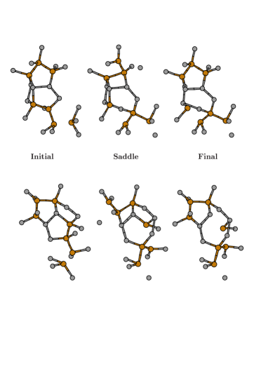
FIG. 1.: An event in the simulation of amorphous silicon. From left to right, the initial, saddle-point, and final configurations are shown. The top and bottom rows correspond to different viewing angles of the same event. Dark atoms change their bonding environment during the event; light atoms are nearest-neighbours of the dark atoms. Activation energy: 5.74 eV, energy difference from initial to final configuration: 2.30 eV.

the configuration reaches a stable energy. To obtain a low-energy configuration, we use the standard Metropolis algorithm where a new configuration is accepted with probability 1 if the energy is lower than that in the original configuration, otherwise with probability $\exp(-\Delta E/k_{B}T)$. The temperature as such is fictitious and we find that $k_{B}T=0.25$ gives satisfactory results. As in Ref. [7], we use a modified Stillinger-Weber[23] interaction potential with a three-body force twice the original value to remove the liquid-like features of the amorphous phase associated with the original SW.

One event obtained in the relaxed structure is shown in Figure 1 from two difference angles. In the bottom representation, we can see how the configuration passes from three five-membered rings (initial) to one five- and one eight-membered ring (final). In the process, four bonds are broken and four are created, preserving the total coordination, and the displacement incurred by the atoms is 2.3 Å. This event has an activation energy of 5.74 eV and the final configuration is 2.30 eV higher than the initial one.

For silica glass, we use a 576-atom configuration relaxed from the melt using molecular dynamics [24]. The initial relaxation was done using the full Vashishta et al. potential[25] while ART was applied using a screened version of the same potential.[26] Figure 2 shows an event in this structure. Because of its more open nature, events

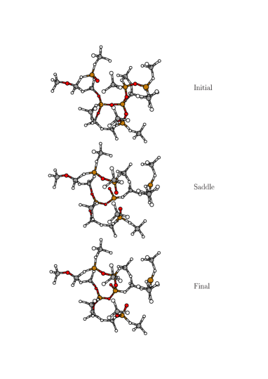
FIG. 2.: An event in the simulation of silica glass. From top to bottom, the initial, saddle-point, and final configurations are shown. Large circles represent Si, small ones O atoms. Dark atoms either change their bonding environment or move by more than 0.75 Å during the event; light atoms are near-neighbours of the dark atoms. Activation energy: 10.84 eV, energy difference from initial to final configuration: 4.25 eV.

in silica tend to involve more atoms than in amorphous silicon. Total atomic displacement between initial and final configurations is 6.8 Å with three broken and two created bonds and many tens of atoms involved at a lower degree during the activation and relaxation phases. The activation energy is considerable, at 10.84 eV, with the new configuration 4.25 eV higher in energy than the initial one.

The characterization of events both in a-Si and g-SiO₂ is difficult: although each event normally involves less than 10 to 12 bonds being broken or created, many more atoms can move significantly, rendering visualization complicated. We are currently working on a systematic study of events in both materials.

V Conclusion

By defining events directly in the configurational energy landscape, the activation-relaxation technique provides a generic approach to study relaxation in complex systems such as glassy and amorphous materials, polymers, and clusters. Real space moves are determined by the system itself and represent the most likely physical trajectories followed during relaxation. ART is much less sensitive to the slowing down caused by increasing activation energy barriers than standard MC and MD approaches.

Already ART has produced results which could not be achieved via other techniques: it has produced well-relaxed samples of a-Si,[7] a-GaAs,[8, 9] Ni₈₀P₂₀, [7] and minimum-energy configurations of clusters of Lennard-Jones particles.[10] The examples of events presented here demonstrate that ART can easily reach regions of the energy landscape which are difficult to sample using more standard techniques. This paper provides the necessary description of the algorithm to allow for a rapid application of ART to a wide range of problems.

VI Acknowledgements

We acknowledge useful and interesting discussions about ART with J. P. K. Doye, M. I. Dykman, S. W. de Leeuw, and V. Smelyanski, and partial support by the Stichting FOM (Fundamenteel Onderzoek der Materie) under the MPR program.

REFERENCES

- [1] Permanent address: Department of Physics and Astronomy, Ohio University, Athens, OH, 45701 USA; e-mail: mousseau@helios.phy.ohiou.edu.
- [2] E-mail: barkema@hlrz.kfa-juelich.de.
- [3] A. F. Voter, Phys. Rev. Lett. 78, 3908 (1997).
- [4] See, for example, references in Simulation of liquids and solids, G. Ciccotti, D. Frenkel and I.R. McDonald, Eds., North-Holland (1987).
- [5] F. Wooten, K. Winer and D. Weaire, Phys. Rev. Lett. 54, 1392 (1985).
- [6] R.H. Swendsen and J.-S. Wang, Phys. Rev. Lett. 58, 86 (1987).
- [7] G. T. Barkema and N. Mousseau, Phys. Rev. Lett 77, 4358 (1996).
- [8] N. Mousseau and L. J. Lewis, Phys. Rev. Lett 78, 1484 (1997).
- [9] N. Mousseau and L. J. Lewis, Phys. Rev. B, 15 Oct. 1997 (tentative date).
- [10] J.P.K. Doye and D.J. Wales, Z. Phys. D 40, 194 (1997).
- [11] As was shown recently (J.P.K. Doye and D.J. Wales, preprint), a complete description of the dynamics requires, besides the energetic aspects, a careful consideration of the entropic effects. In principle, entropic effects can be incorporated in ART. A calculation of vibrational thermodynamical properties is however computer-intensive and at the moment cannot feasibly be integrated into the ART scheme.
- [12] The saddle-points considered here are first-order, i.e. only one eigenvalue of the Hessian matrix —the second-derivative of the configurational energy— is negative and all others positive. In other words, the saddle-point is a configurational energy maximum along one direction, that of the trajectory, and a minimum in all remaining directions. This restriction stems from the observation that, except for very non-generic networks, if in any direction perpendicular to the trajectory the force were non-zero or the eigenvalue of the Hessian negative, a trajectory with a lower activation energy would be found by moving in either direction.
- [13] W.H. Press et al., Numerical Recipes, Cambridge University Press, Cambridge, 1988.
- [14] See, for example, R. S. Berry, H. L. Davis and T. L. Beck, Chem. Phys. Lett. 147, 13 (1988); V. Ivanova and E. A. Carter, J. Chem. Phys. 98, 6377 (1993).
- [15] M. J. Rothman and L. L. Lohr Jr., Chem. Phys. Lett. 70, 405 (1980).
- [16] S. F. Chekmarev, Chem. Phys. Lett. 227, 354 (1994).
- [17] C. J. Cerjan and W. H. Miller, J. Chem. Phys. 75, 2800 (1981).
- [18] J. Simons, P. Jorgensen, H. Taylor and J. Ozment, J. Phys. Chem. 87, 2745 (1983).
- [19] M. I. Dykman, P. V. E. McClintock, V. N. Smelyanski, N. D. Stein and N. G. Stocks, Phys. Rev. Lett. 68, 2718 (1992).
- [20] Besides the atomic coordinates, it is also possible to include additional degrees of freedom in the vector on which ART is applied. For some very dense materials, e.g., metallic glasses, relaxation may be improved significantly by allowing the volume to vary also.
- [21] D. J. Wales and J. P. K. Doye, J. Chem. Phys 106, 5296 (1997).
- [22] P. Steinhardt, R. Alben, and D. Weaire, J. Non-cryst. Sol. 15, 199 (1974).
- [23] F. H. Stillinger and T. A. Weber, Phys. Rev. B 31, 5262 (1985).
- [24] J. V. L. Beckers, unpublished.
- [25] P. Vashishta, R. K. Kalia, J. P . Rino and I. Ebbsjö, Phys. Rev. B 41, 12 197 (1990).
- [26] A. Nakano, L. Bi, R. K. Kalia and P. Vashishta, Phys. Rev. B 49, 9441 (1994).