Finite size effects as the explanation of “freezing” in vortex liquids

Abstract

We investigate the effect of thermal fluctuations on the (mean-field) Abrikosov phase. The lower critical dimension of the superconducting phase is three, indicating the absence of the Abrikosov phase for dimensions $d\leq 3$. Within the $d=3$ vortex liquid, the phase correlation length $\ell_{\parallel}$ along the magnetic field direction grows exponentially rapidly as the temperature is lowered. For a finite bulk system, there is a 3D-2D crossover effect when $\ell_{\parallel}$ becomes comparable to the sample thickness. Such a crossover effect takes place over a very narrow temperature interval and mimics the “first order transition” seen in experiments on clean ${\rm YBa_{2}Cu_{3}O_{7-\delta}}$ (YBCO) and ${\rm Bi_{2}Sr_{2}CaCu_{2}O_{8}}$ (BSCCO) crystals. We calculate the jumps in the entropy, magnetization and specific heat due to the crossover and find reasonably good agreement with experiments on both YBCO and BSCCO.

I Introduction

Abrikosov’s mean-field treatment of conventional Type II superconductors in a magnetic field is very accurate [1] because of their extremely narrow critical regime. In this approximation, the superconducting triangular vortex crystal melts into a resistive vortex liquid via a continuous phase transition. However because of the strong thermal fluctuations about the mean-field solution in high $T_{c}$ superconductors (HTSC) such as YBCO and BSCCO, the nature of the transformation between the superconducting and the normal phase (the vortex liquid), and even the very existence of the mixed phase itself has became an issue of great interest and complexity.

Evidence for a first order melting phase transition from vortex crystal to vortex liquid has been found in recent magnetization measurements on clean crystals of YBCO [2, 3] and BSCCO[4]. The magnetization jump $\Delta M$ associated with the melting is found to be about $3\times 10^{-5}$T at $4$T for YBCO and $4\times 10^{-5}$T at $5\times 10^{-3}$T for BSCCO. By measuring the position of the phase boundary in the $H$-$T$ plane, and assuming a first order phase transition, one can obtain the entropy jump per vortex per CuO layer $\Delta S$ via the Clausius-Clapeyron equation:

$$\frac{\Delta S}{\Delta M}=-\frac{s\Phi_{0}}{B}\frac{dH_{m}(T)}{dT}~{},$$ (1)

where $B$, $s$ and $H_{m}(T)$ are magnetic induction along the $c$-axis, layer spacing and melting line respectively and $\Phi_{0}$ is the flux quantum. For YBCO, $\Delta S$ is calculated to be $0.6k_{B}$/layer/vortex at $4$T[3]. For BSCCO, $\Delta S$ is calculated to be much higher: about $2k_{B}$/layer/vortex at $1\times 10^{-4}$T, and rapidly growing as the temperature approaches $T_{c}$[4]. Recently, both the magnetization jump and the latent heat have been measured on the same YBCO crystal. While Schilling et al. [5] confirmed that the jumps in entropy/vortex/layer and magnetization satisfied the Clausius-Clapeyron equation, Junod et al. [6] found less satisfactory agreement, possibly due to sample inhomogeneities. Both sets of authors report a disappearance of the entropy jump in small fields, which again probably indicates that the experimental data is being affected by sample artifacts.

Recently reported numerical simulations also favor a first order melting transition. Monte Carlo simulations using variants of the 3D XY model give a jump in the entropy[7, 8, 9]. Sasik and Stroud’s 3D Monte Carlo simulation within the lowest Landau level (LLL) approximation[10] (when corrected for an erroneous definition of $\Delta S$) and that of Hu and MacDonald[11] yield estimates of $\Delta S\approx 0.6k_{B}$/layer/vortex, in good agreement with YBCO experiments. However, the results from these simulations in the LLL scheme should be treated with caution: they were performed using quasi-periodic boundary conditions, which imposes an effective (spurious) pinning potential on the vortex motion[12]. A good example of the problem of using the quasi-periodic boundary condition is the case of two-dimensional (2D) (thin film) simulations within the LLL approximation: authors who use quasi-periodic boundary conditions see first order vortex melting [13, 14, 15, 16, 17], whereas simulations in which the 2D vortices move on the surface of a sphere [18, 12], which involves no spurious pinning potential, see no phase transition at all! There is also no experimental evidence that thin film superconductors undergo a first order melting phase transition. A detailed discussion of this topic has been given in Ref. [12].

On the theoretical front, it has been thought for a long time that the Abrikosov lattice will melt into a vortex liquid, and that the phase transition will be first order[19]. However, there is as yet no detailed melting theory. Over the years, many theoretical investigations based on the melting scenario have relied upon the Lindemann criterion: when the spatial fluctuations of a vortex due to thermal excitations become some fraction $c_{L}$ of the vortex lattice spacing, the lattice melts. The Lindemann number $c_{L}$ is usually in the range 0.2–0.4[20]. It has also been suggested that the mechanism behind the apparent first order phase transition is the decoupling of the vortex-lines to pancakes[21]. However, this does not explain the disappearance at the transition of the crystalline order seen in neutron scattering experiments [22].

On the other hand, it is well known that the mean-field Abrikosov solution is unstable against long wavelength thermal excitation of the shear modes of the vortex lattice in both the physical dimensions $d=2$ and $3$ [23, 24]. By calculating the off-diagonal long range order (ODLRO) in the low temperature regime, it has been shown that the lower critical dimension $d_{LC}$ of the mixed phase is three for extreme Type II superconductors ($\kappa>>1$) in an external magnetic field[25]. (The lower critical dimension of an ordered phase is the spatial dimension at and below which a system can no longer sustain the long range order associated with that phase at non-zero temperature). It was suggested therefore that thermal fluctuations will modify the mean-field phase diagram as follows: for $d=2$, the normal vortex liquid is the only thermodynamic phase. For $d=3$, there are only the Meissner and the normal vortex liquid phases. This theoretical scenario for $d=3$ is seemingly at odds with the overwhelming experimental and numerical evidence for a first order melting transition as outlined above, and hence has attracted little attention.

Recently, however, one of us [26] has proposed that the apparent first order melting transition of a vortex crystal to a liquid may be a signature of a finite size effect rather than a genuine thermodynamic phase transition. This idea is based on an extension of Refs. [24] and [25]. In this picture for $d=3$, there exits only one true thermodynamic phase, the vortex liquid phase, characterized by two length scales $\ell_{\parallel}$ and $\ell_{\perp}$; $\ell_{\parallel}$ measures the phase correlation length along the magnetic field direction, and $\ell_{\perp}$ is the range of the (short-range) crystalline order. Both $\ell_{\parallel}$ and $\ell_{\perp}$ are growing exponentially rapidly as the temperature is lowered, but they only become infinite at zero temperature. There is no phase transition to an ordered phase at any finite temperature. This scenario is that of zero temperature scaling[18, 25, 26]. For a finite system, the rapid growth of $\ell_{\parallel}$ and $\ell_{\perp}$ as the temperature is lowered has profound consequences. For a bulk sample with a slab geometry and the field along the $c$-axis, the vortex liquid phase becomes phase correlated along the field direction upon cooling when $\ell_{\parallel}$ reaches the sample thickness $L_{z}$. Then one has phase correlation right across the sample. The behavior of the system then crosses sharply over from that of a 3D vortex liquid to that of a 2D vortex liquid [27]. Such a crossover effect can explain the sudden drop in the $c$-axis resistivity [26]. We will show later that this crossover can quantitatively explain the apparent jumps in the entropy and magnetization of the system observed in experiments. In this simple scenario there is no melting phase transition and a vortex crystal phase does not occur.

The rapid growth of the $c$-axis phase correlation may have already been seen in flux transformer experiments on clean YBCO crystals[28]. Right at the point where the apparent first order melting transition occurs, the voltage difference between various points on the top and bottom of the sample are as if the flux lines moved as rigid rods, indicating phase coherence across the sample thickness. (We acknowledge that a growing $c$-axis conductivity can also produce the same behavior without any substantial degree of phase coherence being present). Recent numerical simulations in frustrated Villain[9], XY [8] and LLL [29] models have reported rapidly growing phase coherence along the $c$-axis upon cooling. With a conventional first order phase transition picture, it is difficult to explain the presence of such a growing length scale at the transition. In addition, the jumps in the magnetization and entropy in Refs. [3] and [30] are actually rounded as functions of magnetic field and temperature. The width of the transition has been calculated within the crossover approach[26], and is in good agreement with data. If there were a genuine first order transition this rounding has to be explained on the basis of a sample artifact etc.

In this paper, we shall follow the zero temperature scaling idea and focus on the growing length scale and the role of finite size effects. The outline of this paper is as follows: we start by describing the LLL approximation based on the the work of Eilenberger [31] and use it to study anharmonic fluctuations in the Abrikosov phase. We then reproduce in Section III the result that $d_{LC}$ of the mixed phase is three [23, 24, 25, 26] within the framework of the loop expansion and estimate the growth rate of $\ell_{\parallel}$ and $\ell_{\perp}$ as a function of temperature in three dimensions. We find the 3D-2D crossover line by setting $\ell_{\parallel}\approx L_{z}$, and compare it to the experimental melting line with the Ginzburg number as the fitting parameter. Both YBCO and BSCCO are examined. In Section IV, we argue that the three dimensional form of the free energy crosses over sharply to the two dimensional thin-film form, mimicking the sharp changes in the thermodynamic potential associated with a first order phase transition. We will calculate the jumps in the first derivative of the free energy to find the entropy jump/layer/vortex, $\Delta S_{cr}$ and the magnetization $\Delta M_{cr}$ and compare them with experiment (where the jumps are usually interpretated as being due to a first order phase transition). We will also demonstrate that $\Delta S_{cr}$ and $\Delta M_{cr}$ satisfy the Clausius-Clapeyron equation. With sets of parameters appropriate for YBCO and BSCCO, we will show that our results are in reasonably good agreement with experiments. The effect of weak random disorder, which is always present even in clean crystals, is investigated in Section V. Finally, we will conclude with a summary and discussion in Section VI. Most of the details of the (necessarily) complicated calculations are to be found in Appendices A–D.

II The Model

We start from the Ginzburg-Landau model with a complex superconducting order parameter $\Psi$ for a system with spatial dimension $d$ and in an external magnetic field ${\bf H}_{0}$ along the $(d-2)$ longitudinal directions. It is assumed that the system has an effective anisotropy ${\bf m}=(m_{\perp},m_{\perp},{\bf m}_{\parallel})$. The free energy functional is

$${\cal F}=\int d^{d}r\bigg{[} \alpha|\Psi|^{2}+\sum_{i=1}^{d}\frac{|(-i\hbar\nabla-2eA_{i})\Psi|^{2}}{2m_{i}}$$ (3)

$$+\frac{1}{2}\beta|\Psi|^{4}+\frac{|{\bf B}-\mu_{0}{\bf H}_{0}|^{2}}{2\mu_{0}}\bigg{]},$$

where $\alpha\propto(T-T_{c})$ and $\beta$ is taken to be a constant. The magnetic induction ${\bf B}=\nabla\times{\bf A}$ is assumed to be uniform inside the bulk of the system and parallel to ${\bf H}_{0}$. This approximation is valid for an extreme Type II (GL parameter $\kappa>>1$) superconductor where the fluctuations in the vector potential ${\bf A}$ are negligible compared to those of the order parameter. Choosing a Landau gauge ${\bf A}=B(-y,0,0)$ and restricting the fluctuations of the order parameter to the LLL subspace, the free energy functional is reduced to:

$${\cal F}_{LLL}=\int d^{d}r\left[\alpha_{H}|\Psi|^{2}+\frac{1}{2}\beta_{\kappa}|\Psi|^{4}+\frac{\hbar^{2}}{2m_{\parallel}}\bigg{|}\frac{\partial\Psi}{\partial{\bf z}}\bigg{|}^{2}\right],$$ (4)

where $\beta_{\kappa}=\beta(1-1/2\kappa^{2})$ and $\alpha_{H}=\alpha+e\hbar\mu_{0}H_{0}/m_{\parallel}$. $\alpha_{H}=0$ defines the mean-field $H_{c2}$ line below which the Abrikosov mean-field solution can be written as[31]

$$\Psi_{0} = \alpha_{0}\varphi({\bf r}|0),$$ (5)

$$\varphi({\bf r}|0) = \left(2\eta\right)^{1/4}\exp\left(-\frac{y^{2}}{2\ell^{2}}\right)\vartheta_{3}\left(\frac{\pi(x+iy)}{\ell_{0}}\bigg{|}\zeta+i\eta\right).$$ (6)

$\Psi_{0}$ has zeros which form a triangular lattice with the fundamental unit cell spanned by the vectors ${\bf r}_{\rm I}=(1,0)\ell_{0}$ and ${\bf r}_{\rm II}=(\zeta=1/2,\eta=\sqrt{3}/2)\ell_{0}$. $\vartheta_{3}$ is a Jacobian theta function and $\ell=\sqrt{\hbar/2eB}$ is the magnetic length. The spacing of the vortices $\ell_{0}$ is given by the flux quantization condition $\eta\ell_{0}^{2}=2\pi\ell^{2}$. For a system with volume $V=L_{x}L_{y}L_{z}^{(d-2)}$, the number of vortices is $N_{\phi}=L_{x}L_{y}/(2\pi\ell^{2})$. $\Psi_{0}$ minimizes the free energy ${\cal F}_{LLL}$ at the value ${F}_{MF}=-|\alpha_{H}|^{2}V/2\beta_{\kappa}\beta_{A}$, with $\alpha_{0}=\sqrt{|\alpha_{H}|/\beta_{\kappa}\beta_{A}}$, and $\beta_{A}=1.1596\dots$ is the Abrikosov number for the triangular lattice. Following Eilenberger [31, 23], we construct an orthonormal basis set for the $N_{\phi}$-fold degenerate ground states of the operator $(-i\hbar{\bf\nabla}-2e{\bf A})^{2}$, {$\Psi_{{\bf p}}=e^{i{\bf q}.{\bf z}}\varphi({\bf r}|{\bf r}_{k})$}, of which $\Psi_{0}$ is a member. Each basis is labelled by a vector ${\bf p}=({\bf k},{\bf q})$ where ${\bf q}$ is the $(d-2)$ dimensional longitudinal vector and ${\bf k}$ is a two dimensional vector confined to the first Brillouin zone (BZ) associated with the ideal triangular lattice. The basis states can be generated using the relation: $\varphi({\bf r}|{\bf r}_{k})=e^{ik_{x}x}\varphi({\bf r}+{\bf r}_{k}|0)$ for ${\bf r}_{k}=(x_{k}+iy_{k})\equiv\ell^{2}(k_{y}-ik_{x})$. The normalization of $\varphi({\bf r}|{\bf r}_{k})$ is taken to be $\overline{|\varphi({\bf r}|{\bf r}_{k})|^{2}}=1$, where the overline denotes a spatial average over the unit cell. In each of the $(d-2)$ longitudinal dimensions, the allowed values of $q$ are integral multiples of $2\pi/L_{z}$ and there are $N_{z}=L_{z}/s$ of them, where $N_{z}$ is the number of layers. The number of allowed ${\bf r}_{k}$ is just $N_{\phi}$. Therefore, the total number of degrees of freedom in a set of {$\Psi_{\bf p}$} is $N_{\phi}N_{z}^{(d-2)}$. To simplify notation, we will drop the bold type on the vectors ${\bf p}$, ${\bf k}$ and ${\bf q}$ henceforth.

Next we set up the standard formalism for perturbation expansion around the condensed mode[32]. Since the functional in Eq. (3) is not translationally invariant, the thermal average of $\Psi$ is spatially inhomogeneous and it is convenient to define a spatially averaged quantity $\tilde{\alpha}$ by $\tilde{\alpha}^{2}=\overline{|<\Psi>|^{2}}$. At mean-field level, $\tilde{\alpha}=\alpha_{0}$. Writing the fluctuating order parameter around $\Psi_{0}$ as

   

$$\Psi = \tilde{\alpha}\varphi({\bf r}|0)+\delta\Psi$$ (7)

$$\delta\Psi = \frac{1}{\sqrt{V}}\sum_{p}\left(\frac{I^{*}(0,0|k,-k)}{|I(0,0|k,-k)|}\right)^{1/2}c_{p}\exp(iq.z)\varphi({\bf r}|{\bf r}_{k}),$$ (8)

$$I(k_{1},k_{2}|k_{3},k_{4}) = \frac{1}{\beta_{A}A}\int_{\rm cell}d^{2}r\varphi^{*}({\bf r}|{\bf r}_{k_{1}})\varphi^{*}({\bf r}|{\bf r}_{k_{2}})\varphi({\bf r}|{\bf r}_{k_{3}})\varphi({\bf r}|{\bf r}_{k_{4}}).$$ (9)

  

Implicit in the definition Eq. (9) is the conservation of momentum $\delta_{k_{1}+k_{2},k_{3}+k_{4}}$, and the transverse integration is over the primitive unit cell of area $A$. $I(k_{1},k_{2}|k_{3},k_{4})$ can be conveniently expressed in terms of lattice sums (see Appendix D). Substituting Eq. (8) into Eq. (4), we find that the free energy to quadratic order in $c_{p}$ is given by

$${\cal F}_{2} = {\cal F}_{MF}+\frac{1}{2}\sum_{p}\left(\begin{array}[]{cc}c_{p}&c_{-p}^{*}\end{array}\right)\left(\begin{array}[]{cc}\Omega_{p}&\Lambda_{p}\\ \Lambda_{p}&\Omega_{p}\\ \end{array}\right)\left(\begin{array}[]{c}c_{p}^{*}\\ c_{-p}\\ \end{array}\right)$$ (15)

where

$$\Omega_{p} = \left(-|\alpha_{H}|+2\beta_{\kappa}\tilde{\alpha}^{2}I(0,k|0,k)+\frac{\hbar^{2}q^{2}}{2m_{\parallel}}\right),$$ (16)

$$\Lambda_{p} = \beta_{\kappa}\tilde{\alpha}^{2}|I(0,0|k,-k)|.$$ (17)

Eq. (15) can be diagonalized as

$${\cal F}_{2}={\cal F}_{MF}+\frac{1}{2}\sum_{p}\left(E_{+}|b_{p}|^{2}+E_{-}|a_{p}|^{2}\right)$$ (18)

with the eigenvalues $E_{\pm}$ and their corresponding normalised eigenvectors ${\bf e}_{\pm}$:

$$E_{\pm} = \Omega_{p}\pm\Lambda_{p}=|\alpha_{H}|\left[\frac{\tilde{\alpha}^{2}}{\alpha_{0}^{2}}(\epsilon_{\pm}+1)-1+\xi_{\parallel}^{2}q^{2}\right],$$ (19)

$${\bf e}_{+} = \frac{1}{\sqrt{2}}\left(\begin{array}[]{c}1\\ 1\\ \end{array}\right),~{}~{}~{}~{}~{}~{}~{}{\bf e}_{-}=\frac{1}{\sqrt{2}}\left(\begin{array}[]{c}1\\ -1\\ \end{array}\right),$$ (24)

where $\epsilon_{\pm}=2I(0,k|0,k)\pm|I(0,0|k,-k)|-1$, and $\xi_{\parallel}=(\hbar^{2}/2m_{\parallel}|\alpha_{H}|)^{1/2}$ is the mean-field correlation length in each of the $(d-2)$ dimensions. The form of Eq. (24) implies that the variable $c_{p}$ can be written as $c_{p}=(ia_{p}+b_{p})/\sqrt{2}$ provided $a_{-p}=a_{p}^{*}$ and $b_{-p}=b_{p}^{*}$ where the complex variables $a_{p}$ and $b_{p}$ measure the amount of soft or hard mode generated by the thermal fluctuations. The number of degree of freedom for each mode is $N_{\phi}N_{z}^{(d-2)}$. The soft mode and hard mode propagators are obtained to lowest order from Eq. (18) and are given respectively by

$$G_{a}(p) = <a_{p}a_{p}^{*}>=\frac{k_{B}T}{|\alpha_{H}|(\epsilon_{-}+\xi_{\parallel}^{2}q^{2})},$$ (25)

$$G_{b}(p) = <b_{p}b_{p}^{*}>=\frac{k_{B}T}{|\alpha_{H}|(\epsilon_{+}+\xi_{\parallel}^{2}q^{2})}.$$ (26)

The soft and hard modes are so-called because of the asymptotic behavior for small $k$: $\epsilon_{-}(k)\sim k^{4}$ and $\epsilon_{+}(k)\sim 2$ (see Appendix D). The consequences of this $k$-dependence of $\epsilon_{-}(k)$ for the lower critical dimension $d_{LC}$ of the system will be discussed in more detail later.

We shall introduce a fictitious source field $J$ into the LLL functional in Eq. (4) such that

$${\cal F^{\prime}}={\cal F}_{LLL}-\int d^{d}r\left(J\varphi({\bf r}|0)\Psi^{*}+c.c\right).$$ (27)

Below $T_{c}$, $J$ singles out $\Psi_{0}\propto\varphi({\bf r}|0)$ as the condensed mode. All results will finally be evaluated at $J=0$. We rewrite $\delta\Psi$ in terms of $a_{p}$ and $b_{p}$ as:

$$\delta\Psi = \frac{b_{0}}{\sqrt{2V}}\varphi({\bf r}|0)+\frac{1}{\sqrt{V}}\sum_{p\neq 0}(ia_{p}+b_{p})Q_{k}e^{iq.z}\varphi({\bf r}|{\bf r}_{k}),$$ (28)

where

$$Q_{k} = \left(\frac{I^{*}(0,0|k,-k)}{2|I(0,0|k,-k)|}\right)^{1/2}.$$ (29)

The term ($b_{0}$ is real) which renormalizes the amplitude of the condensed mode $\varphi({\bf r}|0)$ has been separated out for reasons which will be clear when calculating the equation of state in Section III. The sum $p\neq 0$ implies that except ($q,k$)=($0,0$), $q$ takes on all momenta in the $(d-2)$ longitudinal space, and $k$ takes on all the permitted values in the whole of the first BZ. Expanding Eq. (27) using Eq. (28), we obtain the free energy functional

   

$${\cal F^{\prime}} = V\beta_{\kappa}\beta_{A}(-\alpha_{0}^{2}\tilde{\alpha}^{2}+\tilde{\alpha}^{4}/2)-2JV(\tilde{\alpha}+b_{0}/\sqrt{2V})$$ (36)

$$+\beta_{\kappa}\beta_{A}\left[\sqrt{2V}b_{0}(-\tilde{\alpha}\alpha_{0}^{2}+\tilde{\alpha}^{3})+\frac{1}{2}b_{0}^{2}(-\alpha_{0}^{2}+3\tilde{\alpha}^{2})+\frac{\tilde{\alpha}b_{0}^{3}}{\sqrt{2V}}+\frac{b_{0}^{4}}{8V}\right]$$

$$+\frac{1}{2}\sum_{p\neq 0}|\alpha_{H}|\left\{|a_{p}|^{2}\left[\frac{\tilde{\alpha}^{2}}{\alpha_{0}^{2}}(\epsilon_{-}(k)+1)-1+\xi_{\parallel}^{2}q^{2}\right]+|b_{p}|^{2}\left[\frac{\tilde{\alpha}^{2}}{\alpha_{0}^{2}}(\epsilon_{+}(k)+1)-1+\xi_{\parallel}^{2}q^{2}\right]\right\}$$

$$+\frac{\beta_{\kappa}\beta_{A}}{2V}\left(\frac{1}{2}b_{0}^{2}+\sqrt{2V}b_{0}\tilde{\alpha}\right)\sum_{p\neq 0}\left[\left(\epsilon_{-}(k)+1\right)|a_{p}|^{2}+\left(\epsilon_{+}(k)+1\right)|b_{p}|^{2}\right]$$

$$+\frac{2}{V}\beta_{\kappa}\beta_{A}(\tilde{\alpha}\sqrt{2V}+b_{0})\sum_{p_{i}\neq 0}\Big{[}F(0,p_{1}|p_{2},p_{3})(b_{p_{1}}^{*}b_{p_{2}}b_{p_{3}}+2a_{p_{1}}^{*}b_{p_{2}}a_{p_{3}}-b_{p_{1}}^{*}a_{p_{2}}a_{p_{3}})\Big{]},$$

$$+\frac{\beta_{\kappa}\beta_{A}}{2V}\sum_{p_{i}\neq 0}\Big{[}F(p_{1},p_{2}|p_{3},p_{4})\left(a_{p_{1}}^{*}a_{p_{2}}^{*}a_{p_{3}}a_{p_{4}}+b_{p_{1}}^{*}b_{p_{2}}^{*}b_{p_{3}}b_{p_{4}}+4a_{p_{1}}^{*}b_{p_{2}}^{*}a_{p_{3}}b_{p_{4}}\right)$$

$$~{}~{}~{}~{}~{}~{}~{}~{}~{}~{}~{}~{}~{}~{}~{}~{}~{}-2F(p_{1},-p_{2}|p_{3},-p_{4})b_{p_{1}}^{*}b_{p_{2}}a_{p_{3}}a_{p_{4}}^{*}\Big{]}$$

where

$$F(p_{1},p_{2}|p_{3},p_{4})=\delta_{q_{1}+q_{2},q_{3}+q_{4}}Re[Q_{k_{1}}^{*}Q_{k2}^{*}Q_{k_{3}}Q_{k_{4}}I(k_{1},k_{2}|k_{3},k_{4})].$$ (37)

  

In Eq. (36), the sum of $p_{i}$ is over the whole cell subject to the constraints on $a_{p}$ and $b_{p}$. For the practical purpose of perturbation calculation that follows, it is most convenient to impose the constraints explicitly and sum $p_{i}$ over half over the $d$-dimensional BZ (i.e. $k$ is restricted to half of the two-dimensional BZ and $q$ takes on all allowed momenta).

The low-temperature free energy functional Eq. (36) can be characterised by an effective temperature ${\tilde{T}}=\beta_{\kappa}k_{B}T/(2\ell^{2}\xi_{\parallel}^{d-2}|\alpha_{H}|^{2})$, which is related to another popular variable $\alpha_{T}$ via ${\tilde{T}}=4\pi/|\alpha_{T}|^{3/2}$ for $d=3$. For $d=2$, we define ${\tilde{T}}_{2D}=\beta_{\kappa}k_{B}T/2\ell^{2}L_{z}|\alpha_{H}|^{2}=\pi/|\alpha_{2T}|^{2}$. The low and high temperature limits are represented by ${\tilde{T}}\rightarrow 0$ or $\alpha_{T}(\alpha_{2T})\rightarrow-\infty$, and by ${\tilde{T}}\rightarrow\infty$ or $\alpha_{T}(\alpha_{2T}\rightarrow\infty)$ respectively. Also useful in the following discussion is the definition of $\alpha_{T}=-(2/Gi)^{1/3}(ht)^{-2/3}(1-h-t)$, where $t=T/T_{c}$ and $h=B/B_{c2}(0)$. $Gi$ is the Ginzburg number defined in Ref. [20]. $T_{c}$ and $B_{c2}(0)$ are the zero field transition temperature and the linear extrapolation of $H_{c2}(T)$ to zero temperature respectively.

III The Equation of State

One of the chief aims of this paper is to carry out a loop expansion around the mean-field Abrikosov solution—beyond the Gaussian approximation previously studied[31, 23]—in fact to two loop order. This loop expansion is well known in the O(n) model[33, 32]. We stress that it is a systematic perturbative approach involving no ad hoc Ansatz (such as was employed in Ref.[34]). We shall first calculate the equation of state by finding what value of $\tilde{\alpha}$ makes $<b_{0}>=0$. Within the Gaussian approximation, this just corresponds to putting to zero the coefficient of $b_{0}$ in the functional Eq. (36) (see diagram ${\cal L}_{1}$ of Fig. 1). This reproduces the mean-field results $\tilde{\alpha}=\alpha_{0}$.

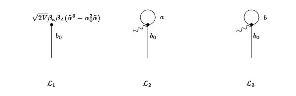
FIG. 1.: Diagrams for determining the equation of state via setting $<b_{0}>={\cal L}_{1}+{\cal L}_{2}+{\cal L}_{3}=0$ up to ${\cal O}(\beta_{\kappa}^{1/2})$. The mean-field value of $\tilde{\alpha}$ is given by ${\cal L}_{1}=0$.

To one loop order, the equation of state involves the tadpole diagrams shown in Fig. 1. Explicit expressions for each diagram are given in Appendix B. The soft and hard mode propagators $G_{a}(p)$ and $G_{b}(p)$ are labelled by $a$ and $b$ respectively. The wavy line in the Feynman diagrams denotes the order parameter $\Psi_{0}$. The thermal averaged value of the amplitude of the order parameter $\tilde{\alpha}=(\overline{|<\Psi>|^{2}})^{1/2}$ will be calculated, where the thermal and spatial averages are denoted by angular bracket and an overline respectively. To one loop order the value of $\tilde{\alpha}$ is

   

$$\tilde{\alpha}^{2} = \alpha_{0}^{2}\left\{1-\frac{\beta_{\kappa}\beta_{A}k_{B}T}{\gamma|\alpha_{H}|(2\pi)^{d}}\int_{BZ}d^{2}k^{\prime}\int d^{d-2}q^{\prime}\left[\frac{\epsilon_{+}(k^{\prime})+1}{\epsilon_{+}(k^{\prime})/\xi_{\parallel}^{2}+q^{\prime 2}}+\frac{\epsilon_{-}(k^{\prime})+1}{\epsilon_{-}(k^{\prime})/\xi_{\parallel}^{2}+q^{\prime 2}}\right]\right\}.$$ (38)

  

where $\gamma=\hbar^{2}/m_{\parallel}$. For $3<d<4$, all integrations are finite without cutoffs. At $d=3$, the integration involving the soft mode (diagram ${\cal L}_{2}$) is infra-red divergent. Let us concentrate on the singular piece of Eq. (38) as $d\rightarrow 3$. Integrating over $q^{\prime}$ first gives:

$$\int_{BZ}d^{2}k^{\prime}\int d^{d-2}q^{\prime}\frac{1}{\epsilon_{-}(k^{\prime})/\xi_{\parallel}^{2}+q^{\prime 2}}$$ (39)

$$\sim \int_{BZ}d^{2}k^{\prime}[\epsilon_{-}(k^{\prime})]^{\frac{d-4}{2}}\Gamma\left(\frac{d-2}{2}\right)\Gamma\left(\frac{4-d}{2}\right)$$ (40)

$$\sim \int^{\Lambda}_{0}k^{\prime 2d-7}dk^{\prime}.$$ (41)

In the last step, a circular BZ of radius $\Lambda$ is assumed. The integral becomes logarithmically divergent at $d=3$ indicating that $d_{LC}=3$. Therefore the Abrikosov phase is unstable against long-wavelength fluctuations in the thermodynamic limit. Such a conclusion has also been reached using a similar analysis within the harmonic approximation [23, 24]. The identification of $\epsilon_{-}(k)\approx c_{66}\ell^{4}k^{4}/2\alpha_{0}^{2}|\alpha_{H}|$ for small $k$ points to the nature of the soft mode which is responsible for the destruction of ODLRO at $d=3$: it is a long-wavelength elastic shear wave. The hard mode, on the other hand, is associated with the compressional mode of the lattice[24]. The low energy excitations about the ground state, i.e. the soft mode, can be described by an effective Hamiltonian [24]:

$${\cal F}_{eff} = {\cal F}_{MF}+\frac{1}{2}\sum_{q,k\in{\rm HC}}\left(c_{66}\ell^{4}k^{4}+\rho_{s}q^{2}\right)\frac{|a_{p}|^{2}}{\alpha_{0}^{2}},$$ (42)

where $\rm HC$ denotes half of the two-dimensional first BZ. $c_{66}$ and $\rho_{s}$ are the elastic shear modulus and superfluid density respectively. The variable $a_{p}$ is just the Fourier component of the phase change $\theta$ of the fluctuating order parameter

$$\theta=\frac{1}{\alpha_{0}\sqrt{2V}}\sum_{p}a_{p}e^{i(k.r+q.{z})}.$$ (43)

(Note that the constraint $a_{p}^{*}=a_{-p}$ in Eq. (43) guarantees that $\theta$ is real.) The soft mode displacements ${\bf u}$ of the vortex lines can be expressed in terms of the derivatives of $\theta$: $u_{x}=-\ell^{2}\partial\theta/\partial y$ and $u_{y}=\ell^{2}\partial\theta/\partial x$ [24]. Since $\nabla.{\bf u}=0$, the flux line motions associated with the soft mode are shear waves[24]. On introducing the dimensionless transverse and longitudinal lengths ${\bf R}=(x/\ell,y/\ell)$ and ${\bf Z}={\bf z}/\xi_{\parallel}$ respectively, Eq. (42) becomes in these dimensionless variables

$$~{}\frac{{\cal F}_{eff}}{k_{B}T}=\frac{{\cal F}_{MF}}{k_{B}T}$$ (44)

$$+\frac{1}{2{\tilde{T}}}\int d^{2}{\bf R}\int d^{d-2}{\bf Z}\left[\tilde{\rho}_{s}\left(\frac{\partial\theta}{\partial{\bf Z}}\right)^{2}+\tilde{c}_{66}\left(\nabla^{2}_{\perp}\theta\right)^{2}\right],$$ (45)

where $\tilde{c}_{66}=\beta_{\kappa}c_{66}/2|\alpha_{H}|^{2}$ and $\tilde{\rho}_{s}=m_{\parallel}\beta_{\kappa}\rho_{s}/\hbar^{2}|\alpha_{H}|$ are the dimensionless shear modulus and superfluid density respectively. At the LLL mean-field level, $\tilde{c}_{66}=0.0885\ldots$ and $\tilde{\rho}_{s}=1/\beta_{A}=0.8624\ldots$ respectively[26].

The length scales $\ell_{\parallel}$ and $\ell_{\perp}$ over which the ODLRO decays can be extracted from the singular piece in Eq. (38). As mentioned before, we expect that $\ell_{\perp}$ is also a measure of the range of the crystalline order in the transverse plane. It will be determined by setting $\tilde{\alpha}=0$ on the left hand side of Eq. (38) and integrating $q\in(0,\infty)$ and then $k\in\sqrt{2}(\ell_{\perp}^{-1},\ell^{-1})$. We obtain

$$\ell_{\perp}\approx\ell\exp({\cal A}|\alpha_{T}|^{3/2}/2),$$ (46)

with ${\cal A}=2\sqrt{\tilde{c}_{66}\tilde{\rho}_{s}}=0.553\ldots$ Similarly, one can extract $\ell_{\parallel}$ by first integrating over $k\in\sqrt{2}(0,\ell^{-1})$ and then $q$ from $2\pi(\ell_{\parallel}^{-1},\xi_{\parallel}^{-1})$. This yields

$$\ell_{\parallel}\approx\xi_{\parallel}\exp\left({\cal A}|\alpha_{T}|^{3/2}\right).$$ (47)

As the temperature drops, $\ell_{\perp}$ and $\ell_{\parallel}$ grow rapidly but only diverge in the zero temperature limit ($\alpha_{T}\rightarrow-\infty$) where true ODLRO order exists. The functional forms for $\ell_{\perp}$ and $\ell_{\parallel}$ have been suggested by one of us[26] using a simple renormalization group argument based on the effective Hamiltonian Eq. (45). However, the number ${\cal A}$ is estimated here for the first time[29]. We acknowledge that our estimate of ${\cal A}$ can only be regarded as an order of magnitude estimate. For example, setting $(\tilde{\alpha}/\alpha_{0})^{2}$ equal to a constant$<$1 rather than zero produces a different value of ${\cal A}$. However, we find that the value of ${\cal A}$ quoted here gives an excellent prediction for the position of the “melting” line in YBCO (see below). Our calculation of the “jumps” in the entropy, magnetization etc. is independent of our estimate of ${\cal A}$, as we express their magnitudes in terms of the measured value of $\alpha_{T}^{*}$ at the “melting” line. In Appendix A, we suggest that only a non-perturbative approach incorporating the topological defects such as entanglements will lead to a quantitative estimate of the coefficient $\cal A$.

For crystals of the shape normally used in the studies of high temperature superconductors, $\ell_{\parallel}$ will grow to the system dimension $L_{z}$ before $\ell_{\perp}$ reaches the transverse dimension $L_{x}$. When this happens, there is phase correlation along the $c$-axis, and the system will then behave as if it were effectively two dimensional. $\ell_{\perp}$ is also growing exponentially, although slower than $\ell_{\parallel}$, and it is expected to be several orders of magnitude times the lattice spacing at the crossover temperature when $\ell_{\parallel}\approx L_{z}$. Therefore, when $\ell_{\parallel}\approx L_{z}$, the system is a vortex liquid with quasi-long range order, which explains the apparent Bragg-like peaks in neutron scattering experiments[22, 35]. The apparent formation of sharp Bragg-like peaks from the rings (expected to be) seen in the structure factor for the vortex liquid phase when the temperature is lowered is usually attributed to the freezing of the vortex liquid to the vortex crystal phase. However, a recent theoretical investigation[36] has found that such a transformation in the structure factor can also take place entirely within the vortex liquid phase in the presence of a weak four-fold symmetric coupling to the underlying crystal. In fact, the angular width of the peaks $\delta\theta$ varies as $\delta\theta\propto\ell_{\perp}^{-1}$ for a given coupling to the underlying crystal. This implies that the width of the peaks should shrink exponentially rapidly when the temperature is lowered.

The mechanism for the 3D to 2D crossover can be illuminated by a “toy” calculation for the 3D vortex liquid. Consider the Hartree-Fock approximation to the propagator in the vortex liquid phase given in Fig. 2. This calculation is normally done for an infinite system, but we shall do for a system of finite width $L_{z}$ to illustrate the 3D-2D crossover mechanism.

FIG. 2.: The Hartree-Fock approximation. The double and single lines denote the renormalized and bare propagators $G(q)$ and $g(q)$ respectively.

The renormalised propagator $G(q)$ (deriving from $<\Psi^{*}({\bf r}^{\prime},{\bf z^{\prime}})\Psi({\bf r},{\bf z})>$) is related to the bare propagator $g(q)=k_{B}T/(\alpha_{H}+\hbar^{2}q^{2}/2m_{\parallel})$ such that the “mass” term $\alpha_{H}$ becomes $G(q)=k_{B}T/(\alpha_{R}+\hbar^{2}q^{2}/2m_{\parallel})$ with

$$\alpha_{R} = \alpha_{H}+\frac{\beta_{\kappa}k_{B}T}{\pi\ell^{2}L_{z}}\sum_{n=-\infty}^{\infty}\frac{1}{\alpha_{R}+(\hbar^{2}/2m_{\parallel})q_{n}^{2}}$$ (48)

$$= \alpha_{H}+\frac{\beta_{\kappa}k_{B}T}{2\pi\ell^{2}}\sqrt{\frac{2m_{\parallel}}{\hbar^{2}\alpha_{R}}}\coth\left(\frac{L_{z}}{\tilde{\xi}_{\parallel}}\right)$$ (49)

where the wavevector $q_{n}=2\pi n/L_{z}$ for a system of finite size $L_{z}$ with periodic boundary condition. $\tilde{\xi}_{\parallel}=(\hbar^{2}/2m_{\parallel}\alpha_{R})^{1/2}$ is the renormalized correlation length along the field direction. By using the asymptotic behavior $\coth(x)\sim 1/x$ for small $x$ and $\coth(x)\sim 1$ for large $x$, one can see that Eq. (49) reduces to the well known results for 2D and 3D (Eqs. (23) and (24) in Ref. [37]) in the limit of $L_{z}<<\tilde{\xi}_{\parallel}$ and $L_{z}>>\tilde{\xi}_{\parallel}$ respectively. Notice that the 2D limit ($L_{z}<<\tilde{\xi}_{\parallel}$) of $\alpha_{R}$ is dominated by just the $n=0$ term in the sums. Although $\tilde{\xi}_{\parallel}$ is not exponentially growing (because $d_{LC}=4$ in this approximation), one can see how the behavior of the system is controlled by the ratio of the length scale $L_{z}$ and $\tilde{\xi}_{\parallel}$, and that in the 2D limit one can proceed as if the flux lines were straight rods.

Returning to the full problem, as the temperature change required to pass from the regime $\ell_{\parallel}\ll L_{z}$ to $\ell_{\parallel}\approx L_{z}$ is very small[26], we believe that the crossover has been mistakenly interpretated as a first order melting phase transition. Later on, we will calculate the sharp step in the magnetization and the entropy/vortex/layer due to this crossover and show that it has many features of a first order phase transition.

First, we shall investigate the position in the $H-T$ phase diagram where the crossover $\ell_{\parallel}\approx L_{z}$ takes place. In dimensionless units this occurs when $\alpha_{T}=\alpha_{T}^{*}$ where

$$\alpha_{T}^{*}\approx-\left[\frac{1}{{\cal A}}\ln\left(\frac{L_{z}}{\xi_{\parallel}}\right)\right]^{2/3}.$$ (50)

For a typical YBCO crystal of thickness 0.2mm and $\xi_{\parallel}\approx 10{\rm\AA}$, we estimate using our estimated value of ${\cal A}$ that the crossover is at around $\alpha_{T}^{*}\approx-7.9$ which agrees with the supposed ‘melting’ line in previous investigations [38, 39]. For the same sample thickness, but using a typical shorter coherence length $\xi_{\parallel}\approx 2.0{\rm\AA}$ appropriate to BSCCO, we find that $\alpha_{T}^{*}\approx-8.9$. Note that the position of the crossover $\alpha_{T}^{*}$ is only weakly (logarithmically) dependent on $\L_{z}/\xi_{\parallel}$, whose dependence on $T$ and $B$ will therefore be neglected in what follows below. The dependence of the parameter $\alpha_{T}^{*}$ on $T$ and $B$ implies that the position of the crossover line in the phase diagram should follow the power law:

$$B_{cr}\approx B_{0}\left(1-\frac{T}{T_{c}}\right)^{n},$$ (51)

where $n=3/2$ and $B_{0}$ is the zero temperature melting magnetic field. Strictly speaking $T_{c}$ is the mean-field transition temperature, and fluctuation effects will make its value slightly different from the measured zero-field transition temperature.

FIG. 3.: The experimental ‘melting’ points fitted with Eq. (51) (solid line) for YBCO and BSCCO. These data are read from the bottom panel of Fig. 5 in Ref. [3] and Fig. 4 in Ref. [4] respectively.

Using the YBCO and BSCCO ‘melting’ data from Refs. [3] and [4] respectively, we find reasonably good fits with $(B_{0},T_{c})\approx$ (140T, 92.9K) and $(B_{0},T_{c})\approx$ (0.1T, 94.3K ) respectively (see Fig. 3). By substituting Eq. (51) into the definition of $\alpha_{T}$, we have

$$\alpha_{T}^{*}\approx-\left(\frac{2}{Gi}\right)^{1/3}\left(\frac{B_{c2}(0)}{B_{0}}\right)^{2/3}.$$ (52)

We can then determine the Ginzburg number $Gi$ of YBCO and BSCCO by comparing Eq. (50) and Eq. (52). Using $B_{c2}(0)\approx 170$T in both cases [40], we obtain $Gi_{{\rm YBCO}}\approx 0.006$ and $Gi_{\rm BSCCO}\approx 8000$. While the former is a widely quoted number for YBCO, the later is about four order of magnitude bigger than the usual value quoted of 0.1. We believe that this might not be unphysical for BSCCO, and the argument is as follows. What we are using is a phenomenological model—the LLL approximation—which is quantitatively useful as long as the effective temperature $\alpha_{T}$ provides a good representation of the true temperature and field dependence. This seems to be the case for YBCO. On the other hand, $B_{0}$ for BSCCO is approximately three orders of magnitude smaller than that of YBCO which suggests that fluctuations effects are enormous and are likely to renormalize the bare parameters of the theory. Effects from the higher Landau level contributions, the quasi-two dimensional behavior of BSCCO and the fluctuations of the vector potential, which have been neglected in this effective model will all act to modify the dependence of $\alpha_{T}$ on temperature and magnetic field away from the simple bare expression for $\alpha_{T}$ as in Eq. (52). So in principle, one also should expect $Gi_{{\rm BSCCO}}$ to be a function of both temperature and magnetic field rather than a constant, as we have done above. However, a qualitatively useful description of BSCCO may be possible if we are prepared to accept a renormalized $Gi$ much larger than the bare $Gi$. Therefore, we will keep an open mind, and proceed to investigate what the effective model can offer in the description of both YBCO and BSCCO. This philosophy seems to have been adopted by other authors as well. In their recent Monte Carlo simulation, Hu and MacDonald[11] had implicitly used a very large $Gi$ in order to fit their numerical results to BSCCO. On the other hand it is possible that the large value of $Gi$ needed to fit the data in BSCCO is really telling us that the mechanism of the two transitions in YBCO and BSCCO are quite different e.g. that the crossover idea applies to YBCO but that there is a genuine first order transition in BSCCO.

Also of some interest is the angular dependence of the crossover line. When the magnetic field is tilted at an angle $\phi$ to the $c$-axis, then the crossover effect will occur at $\ell_{\parallel}\approx L_{z}/\cos(\phi)$. Using the general scaling approach of Blatter et al. [41], the dimensionless temperature scales as (ignoring as before logarithmic corrections)

$$|\alpha_{T}^{*}(\phi)|^{3/2} \approx |\alpha_{T}^{*}(0)|^{3/2}\sqrt{\cos^{2}\phi+\sin^{2}\phi/\Gamma^{2}}$$ (53)

where $\Gamma=\sqrt{m_{\parallel}/m_{\perp}}$ is the anisotropy factor. Throughout the rest of the paper, we will only examine the case of $\phi=0$, i.e. a field along the $c$-axis.

IV Thermodynamics

Although the crossover behavior discussed above is a finite size induced effect rather than a phase transition, we can still associate with it a “jump” in the entropy per vortex per layer $\Delta S_{cr}$ and the magnetization $\Delta M_{cr}$ due to the narrowness of the crossover region. We believe that apparent first order melting signatures like the latent heat and magnetization jumps observed in experiments are in fact due to the entropy and magnetization differences between the 2D and 3D vortex liquid.

Although the jumps in the magnetization and entropy are reported to be sharp, they in fact have a finite width[3, 5, 42]. Such rounding of the jumps is usually attributed to the sample or magnetic field inhomogeneity. However, we can explain such rounding as the natural width of the crossover effect. A simple prescription to estimate the width is to find the small change $\delta\alpha_{T}$ in $\alpha_{T}^{*}$ (set by $\ell_{\parallel}\approx L_{z}$) required for $\ell_{\parallel}\approx 2L_{z}$. Using the definition of $\alpha_{T}$, we obtain $\delta\alpha_{T}/\alpha_{T}\approx(2/3)\delta B/B$. Substituting this into Eq. (50) and using $L_{z}=0.2$mm and $\xi_{\parallel}\approx 10{\rm\AA}$ for YBCO, we get $\delta B/B\approx 0.057$ at a magnetic field of $4.2$T. Using the YBCO magnetization data from Fig. 1 in Ref. [3], we estimate that the width is $\delta B\approx 0.2$T at $B=4.2$. This gives $\delta B/B\approx 0.05$, which is good agreement with the predicted crossover width.

If one can calculate the 2D and 3D free energies $F_{2D}$ and $F_{3D}$ of the vortex liquid phase, then one would naively expect the $\Delta S_{cr}=-(s\Phi_{0}/BV)\partial(F_{3D}-F_{2D})/\partial T$ and $\Delta M_{cr}=-(1/V)\partial(F_{3D}-F_{2D})/\partial H$. However, there are two subtleties involved here and this expectation is not correct. The first of these is a simplification. From their definitions $\alpha_{T}$ and $\alpha_{2T}$ are such that $\alpha_{2T}^{*}=-\sqrt{L_{z}|\alpha_{3T}^{*}|^{3/2}/4\xi_{\parallel}}$. Because $L_{z}\gg\xi_{\parallel}$ for a bulk system, $\alpha_{2T}$ is orders of magnitude larger than $\alpha_{T}$. For YBCO, the crossover occurs at $\alpha_{3T}^{*}\approx-7.9$. For the 2D liquid, this corresponds to $\alpha_{2T}^{*}\approx-1200$ (similar estimates apply to BSCCO). At such a low effective temperature, the behavior of the 2D liquid is basically mean-field like, and fluctuation effects are negligible. With this in mind, the sharp changes in the thermodynamic functions between the two regimes can be obtained by subtracting the mean-field expression from that of the 3D expression. The second subtlety is that not all contributions to the entropy or magnetization are sensitive to the effect of crossover. For example, the short wavelength contributions are not modified when $\ell_{\parallel}$ becomes comparable to $L_{z}$, and so will not contribute to the jumps. Therefore, in calculating the 3D entropy, magnetization and specific heat jumps, we need to examine all contributions and discard the pieces that are continuous over the crossover region.

Before deriving the thermodynamic functions, we would like to specify how we envisage infinitesimal changes in the magnetic field, i.e. taking the derivatives of say, the free energy with respect to the magnetic field. We assume a finite system which is allowed to change its transverse area $L_{x}L_{y}$ so that as the magnetic induction changes, the number of vortices inside the system, $N_{\phi}$ remain constant. The two are related by $N_{\phi}=L_{x}L_{y}/2\pi\ell^{2}$. This framework naturally allows small changes in the magnetic induction without the introduction of extra vortices, and because of its calculational convenience it has also been used in the Monte Carlo simulations of vortices[10, 12, 43].

The total 3D free energy of the system can be written as

$$F = F_{MF}-N_{\phi}\frac{k_{B}TL_{z}\pi}{2\beta_{A}\xi_{\parallel}{\tilde{T}}}{\cal G}({\tilde{T}})$$ (54)

$${\cal G}({\tilde{T}}) = -{\cal E}^{(1)}{\tilde{T}}+{\cal E}^{(2)}{\tilde{T}}^{2}+\dots,$$ (55)

where $F_{MF}$ is the mean-field free energy and ${\cal G}({\tilde{T}})$ is a the 3D dimensionless free energy calculated by expanding about the mean-field solution. ${\cal E}^{(i)}$ is a number given by the $i$-th loop contribution to the dimensionless free energy (see Appendix C). By definition, the total entropy per unit volume is

   

$$S=-\frac{1}{V}\frac{\partial F}{\partial T}=-\frac{1}{V}\frac{\partial F_{MF}}{\partial T}+\frac{N_{\phi}\pi k_{B}L_{z}}{2\beta_{A}V}\left[\frac{{\cal G}({\tilde{T}})}{{\tilde{T}}}\frac{\partial}{\partial T}\left(\frac{T}{\xi_{\parallel}}\right)+\frac{T}{\xi_{\parallel}}\frac{\partial}{\partial T}\left(\frac{{\cal G}({\tilde{T}})}{{\tilde{T}}}\right)\right].$$ (56)

  

The first term corresponds to the mean-field entropy per unit volume. Across the crossover region, the first term inside the square brackets is continuous because both ${\cal G}({\tilde{T}})$ and $\partial(T/\xi_{\parallel})/\partial T$ are continuous. It is the first derivative of ${\cal G}({\tilde{T}})$ in the second term that gives the impression of a discontinuity at the crossover to the 2D regime. Therefore the apparent drop in entropy upon cooling through the crossover region is the total entropy minus all the background pieces (including the mean-field contribution), that are continuous or smoothly varying in the crossover region. Thus, the jump in the entropy per unit volume due to the crossover effect is:

$$\Delta S=\frac{N_{\phi}L_{z}k_{B}T\pi}{2\beta_{A}V\xi_{\parallel}}\frac{\partial}{\partial T}\left[\frac{{\cal G}({\tilde{T}})}{{\tilde{T}}}\right].$$ (57)

Per vortex per layer, the leading term in the loop expansion for the crossover entropy jump is

$$\Delta S_{cr} = \frac{s\pi k_{B}{\cal E}^{(2)}}{2\beta_{A}\xi_{\parallel}}\frac{\partial{\tilde{T}}}{\partial T}$$ (58)

$$\approx \frac{3\pi^{2}sk_{B}{\cal E}^{(2)}}{\beta_{A}\xi_{\parallel}(0)}\left(\frac{2}{Gi}\right)^{1/6}\frac{t^{*2/3}h^{*-1/3}}{|\alpha_{T}^{*}|^{2}},$$ (59)

where the superscript $*$ mean that the quantities are evaluated at the crossover. In the last line, we have used the approximation $1/t^{*}\ll 3/2(1-h^{*}-t^{*})$ in calculating $\partial{\tilde{T}}/\partial T$ at the crossover. (This approximation can be easily justified by comparing the order of magnitude of the two terms using typical YBCO and BSCCO parameters at the crossover. In fact one can establish that $1/t^{*}\ll 3/2(1-h^{*}-t^{*})\ll 1/h^{*}$).

In the same way, we can obtain the magnetization of the system via the definition $M=-(1/V)\partial F/\partial H$. (This means that the magnetization is not just—$<\overline{|\Psi|^{2}}>$ as in the original work of Abrikosov[1]). Using the same argument as before, the relevant crossover magnetization jump arises from the term $\partial[{\cal G}({\tilde{T}})/{\tilde{T}}]/\partial H$. The leading crossover magnetization jump is

$$\Delta M_{cr} = \frac{\pi\mu_{0}Hk_{B}t{\cal E}^{(2)}}{2\beta_{A}\Phi_{0}\xi_{\parallel}}\frac{\partial{\tilde{T}}}{\partial H}$$ (60)

$$\approx \frac{2\pi^{2}k_{B}T_{c}\mu_{0}{\cal E}^{(2)}t^{*4/3}h^{*1/3}}{\beta_{A}\xi_{\parallel}(0)\Phi_{0}|\alpha_{T}^{*}|}\left(\frac{Gi}{2}\right)^{1/6}.$$ (61)

Again, we have used the approximation $1/h^{*}\gg 3/2(1-h^{*}-t^{*})$ in calculating $\partial{\tilde{T}}/\partial H$ at the crossover.

It is now easy to see that $\Delta S_{cr}$ and $\Delta M_{cr}$ satisfy the Clausius-Clapeyron Eq. (1) automatically. The gradient of the crossover $\partial H_{cr}/\partial T$ can determined by differentiating Eq. (51) directly. This apparent thermodynamic consistency in the jumps $\Delta S_{cr}$ and $\Delta M_{cr}$ has been used to argue for the existence of first order melting in YBCO[2, 3, 5] and BSCCO[4]. However, our crossover scenario seems to provide a possible alternative explanation.

How do our expressions for $\Delta M_{cr}$ and $\Delta S_{cr}$ compare with the actual experimental results? Notice that it is the two loop term ${\cal E}^{(2)}$ in the free energy, rather than one loop term ${\cal E}^{(1)}$ which gives the leading order contribution to $\Delta S_{cr}$ and $\Delta M_{cr}$. In order to get an estimate of $\Delta S_{cr}$ and $\Delta M_{cr}$ we need to calculate ${\cal E}^{(2)}$, i.e. evaluate the diagrams shown in Fig. 4.

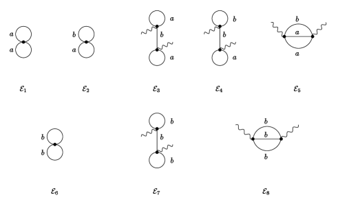
FIG. 4.: Free energy diagrams of ${\cal O}(\beta_{k})$.

Each vertex is ${\cal O}(\beta_{\kappa})$, and each contribution from wavy line is proportional to $\beta_{\kappa}^{-1/2}$, and so all the above diagrams are of the same order. The single and double vertex diagrams have an overall negative and positive sign respectively. $a$ labels the soft mode propagator, which is infra-red divergent at $d=3$. The sum of all diagrams involving the soft mode remains finite although individual diagrams are divergent (see Appendix C). The number ${\cal E}^{(2)}$ is estimated to be $4.4\times 10^{-2}$.

Having found ${\cal E}^{(2)}$, we can evaluate the orders of magnitude of $\Delta S_{cr}$ and $\Delta M_{cr}$ at some typical field. These result should apply to both YBCO and BSCCO provided that the appropriate phenomenological parameters are used to used to model them realistically. For YBCO, we choose $s\approx 10{\rm\AA}$, $\xi_{\parallel}(0)\approx 2.2{\rm\AA}$ and $\alpha_{T}^{*}\approx-7.9$. This give us $\Delta S_{cr}\approx 0.7k_{B}$/layer/vortex and $\Delta M_{cr}\approx 4.0\times 10^{-5}T$ at $4$T. For BSCCO, we use $s\approx 11{\rm\AA}$, $\xi_{\parallel}(0)\approx 1.8{\rm\AA}$ and $\alpha_{T}^{*}\approx-8.9$, and we estimate that $\Delta S_{cr}\approx 1.0k_{B}$/layer/vortex and $\Delta M_{cr}\approx 0.5\times 10^{-4}T$ at $5\times 10^{-3}$T. These results are in good agreement with experiment[4, 3, 5].

FIG. 5.: $\Delta S_{cr}$ and $\Delta M_{cr}$ as a function of $T$ for YBCO and BSCCO. Data points for $\Delta S_{cr}$($\circ$) and $\Delta M_{cr}$($\diamond$) are read from Fig. 4(a) in Ref. [3] and Fig. 5 and 6 in Ref. [4] respectively. Solid lines are theoretical fits using Eq. (61) and Eq. (59) respectively, with material parameters discussed in the text.

More importantly, our crossover results predict that $\Delta S_{cr}\sim h^{*-1/3}\sim(1-t^{*})^{-1/2}$ and $\Delta M_{cr}\sim h^{*1/3}\sim(1-t^{*})^{1/2}$ as $T$ approaches $T_{c}$. Fig. 5 shows the temperature dependence of $\Delta M_{cr}$ and $\Delta S_{cr}$ compared to the experiments using material parameters as previously mentioned. The YBCO and BSCCO data points are read from Welp et al. [3] and Zeldov et al. [4] respectively. Our result for $\Delta M_{cr}$ not only agrees reasonably well with the bulk of the YBCO and BSCCO data, it also accounts for the general temperature dependence quite well. The divergence of $\Delta S_{cr}$ near $T_{c}$ is consistent with the BSCCO data. However, this is apparently at odds with the YBCO data, as Welp et al. [3] see vanishing $\Delta S_{cr}$ as $T\rightarrow T_{c}$. The authors themselves suspect that this is due to the influence of sample inhomogeneity very near $T_{c}$ [3]. In view of this, more weight should perhaps be given to the low temperature points when comparing our results with the data in Fig. 5. We believe that if sample artifacts could be removed, the divergence of $\Delta S_{cr}$ as $T\rightarrow T_{c}$ in YBCO would be revealed.

A consistent picture of even the form of the crossover line is not available from experiments. Zeldov et al. [4] deduced an exponent $n\approx 1.55$ for BSCCO, which is close to the results expected from the crossover mechanism (Eq. (51)). On the other hand, Liang et al. [2] and Welp et al. [3] deduced a YBCO melting line with a smaller slope ($n\approx$ 1.34, 1.36 respectively). The confusion is further exemplified by the YBCO measurement of Nishizaki et al. [44] where a power law appropriate to the London model ($n\approx 2$) was used. They estimated that $\Delta S_{cr}\approx 6k_{B}$ at $1$T and $25k_{B}$ at $3$T. Both the magnitude and the temperature dependence of their results are in total disagreement with our results here and other YBCO measurements[3, 2, 5].

In our approach, there is no qualitative difference between YBCO and BSCCO. They just differ in having vastly different effective values of $Gi$. But our treatment for BSCCO requires the insertion of a value of $Gi$ hugely renormalized by fluctuation effects. $Gi$ would then be expected to be a function of temperature and field, and not a constant as assumed here. Inserting such temperature and field dependence (if known!) could improve the fits in Fig. 5. Without inclusion of disorder, our model does not explain the vanishing of $\Delta S_{cr}$ at a lower temperature critical point as observed in BSCCO by Zeldov et al. [4] (neither do the melting nor decoupling models). Such behavior is thought to be disorder induced. The effect of random disorder will be discussed in more detail in Section V, and seems consistent with the data of Ref. [4].

The recent advent of reliable calorimetric measurements[30, 6] has also made available specific heat data for comparison. This has motivated us to calculate the leading crossover value for the specific heat jump. The total specific heat capacity is given by

   

$$\frac{C}{T} = \frac{\partial S}{\partial T}=-\frac{1}{V}\frac{\partial^{2}F_{MF}}{\partial T^{2}}+\frac{N_{\phi}L_{z}k_{B}\pi}{2\beta_{A}V}\left[\frac{{\cal G}({\tilde{T}})}{{\tilde{T}}}\frac{\partial^{2}}{\partial T^{2}}\left(\frac{T}{\xi_{\parallel}}\right)+\frac{T}{\xi_{\parallel}}\frac{\partial^{2}}{\partial T^{2}}\left(\frac{{\cal G}({\tilde{T}})}{{\tilde{T}}}\right)+2\frac{\partial}{\partial T}\left(\frac{T}{\xi_{\parallel}}\right)\frac{\partial}{\partial T}\left(\frac{{\cal G}({\tilde{T}})}{{\tilde{T}}}\right)\right].$$ (62)

  

The first term is just the mean-field part of the specific heat. The first term inside the square bracket in Eq. (62) is continuous through the crossover region. Only the last two terms with the derivatives of ${\cal G}$ are sensitive to the crossover and hence contribute to the crossover specific heat jump $\Delta C_{cr}$. After some algebra, we find that to leading order in the loop expansion, per vortex per layer,

$$\frac{\Delta C_{cr}}{T}\approx\frac{9\pi^{2}{\cal E}^{(2)}sh^{-1}}{2\beta_{A}\xi_{\parallel}(0)T_{c}|\alpha_{T}|^{3}}\left(\frac{2}{Gi}\right)^{1/2}k_{B}.$$ (63)

In order to make it more convenient to compare with the experiment of Schilling et al. [30], we convert this result to units of mJ/mole K² using the scale in Fig. 4(b) of Ref. [30] (namely, $1k_{B}$/vortex/layer $\equiv$ 0.6 mJ/mole T K), so Eq. (63) in the units of mJ/mole T K² is given by

$$\frac{\Delta C_{cr}}{T}\approx 0.6\times\frac{9\pi^{2}{\cal E}^{(2)}sB_{c2}(0)}{2\beta_{A}\xi_{\parallel}(0)T_{c}|\alpha_{T}^{*}|^{3}}\left(\frac{2}{Gi}\right)^{1/2}.$$ (64)

Using the appropriate parameters for YBCO, we found that the leading $\Delta C_{cr}/T$ is constant at 0.3 mJ/mole K², which is approximately four times smaller than the data in Fig. 5 of Ref. [30] (see Fig. 6). This discrepancy may be due to our neglect of the higher order terms in the loop expansion. In any case, as a first order approximation, our results give a useful qualitative description of the current experimental data.

FIG. 6.: Specific heat difference due to the crossover from 3D to 2D. Data points with magnetic field parallel to the $c$-axis are read from Fig. 5 of Ref. [30]. The circular and triangular open symbols represent $\Delta C_{cr}/T$ based on specific heat and magnetization measurements respectively. The solid horizontal line is our result using Eq. (64) using a set of parameters appropriate to YBCO.

V Effect of Random disorder

In this section, we investigate the effect of quenched disorder (which is always present even in high quality YBCO and BSCCO crystals), on the order in the Abrikosov phase. The effects of quenched disorder on the “melting” transition of YBCO and BSCCO at high magnetic fields is well documented. We will just mention a few of them here. Safar et al. [45] reported the existence of an “upper critical point” in untwinned YBCO at a high magnetic field beyond which the sharp drop in resistivity disappeared. In a recent report of the specific heat measurements on YBCO, Roulin et al. [42] have suggested that the termination of the “melting line” takes place at about 14T. Using a sensitive local Hall probe, Zeldov et al. [4] also reported similar feature in BSCCO, albeit at a much lower magnetic field (0.038T). It is widely believed that at high magnetic fields the pinning of the vortices by disorder is more effective and the “first order melting transition” is removed[45, 46, 6]. In an illuminating experiment, Fendrich et al. [46] have directly demonstrated that the suppression of the sharp kink in the resistivity drop in YBCO is a disorder-induced effect. They measured and compared the resistivity before and after a controlled introduction, by electron irradiation, of point defects in the sample. Furthermore, they showed that the sharp kinks in the resistivity drop can be recovered by reducing the density of the point defects through subsequent annealing of the sample [46]. At a low magnetic field, disorder is also thought to affect the properties of YBCO. The existence of such “lower critical point” produced by disorder or sample inhomogeneity (by an unknown mechanism) was recently invoked to explain the disappearance of the jumps in magnetization and entropy/vortex/layer in YBCO experiments[3, 5, 6] at low fields.

With this motivation we proceed to investigate the effect of disorder on the Abrikosov phase. For simplicity, we will neglect the effect of thermal fluctuations and focus on very weak spatially varying disorder characterized by a locally varying transition temperature $\tau({\bf r})$. As a first approximation, we adopt the “random $T_{c}$” approach[32, 47], i.e. $\tau({\bf r})$ is assumed to have a Gaussian distribution:

$$\ll\tau({\bf r})\gg = 0,$$ (65)

$$\ll\tau({\bf r})\tau({\bf r}^{\prime})\gg = \frac{W}{2}\delta({\bf r}-{\bf r}^{\prime}),$$ (66)

where $\ll\cdots\gg$ denotes averaging over all $\tau({\bf r})$ configurations. The GL functional in the LLL approximation is given by

$${\cal F}=\int d^{d}r\bigg{\{} \left(\alpha_{H}+\tau({\bf r})\right)|\Psi|^{2}\frac{\hbar^{2}}{2m_{\parallel}}\bigg{|}\frac{\partial\Psi}{\partial{\bf z}}\bigg{|}^{2}$$ (68)

$$+\frac{1}{2}\beta|\Psi|^{4}\bigg{\}}.$$

Our plan is to take the disorder to be weak and investigate the effect of the disorder on the pure system ground state $\Psi_{0}=\alpha_{0}\varphi({\bf r}|0)$. Expanding in terms of $a_{p}$ and $b_{p}$ about this, we obtain the functional up to quadratic order

   

$${\cal F} = {\cal F}_{MF}+\frac{1}{2}\sum_{p}|\alpha_{H}|\left[(\epsilon_{-}+\xi_{\parallel}^{2}q^{2})|a_{p}|^{2}+(\epsilon_{+}+\xi_{\parallel}^{2}q^{2})|b_{p}|^{2}\right]$$ (70)

$$+\frac{2\alpha_{0}}{\sqrt{V}}\sum_{p}\int d^{d}r\left\{\tau({\bf r})Re\left[\left(ia_{p}+b_{p}\right)Q_{k}\varphi^{*}({\bf r}|0)\varphi({\bf r}|{\bf r}_{k})e^{iq.z}\right]\right\},$$

  

where ${\cal F}_{MF}$ is the ground state free energy. The variables $a_{p}$ and $b_{p}$ are now disorder, rather than thermal, induced fluctuation amplitudes in the soft and hard modes respectively. At this order, the minimum free energy is determined by the conditions

$$\frac{\partial{\cal F}}{\partial x_{p}}=0,$$ (71)

where $x_{p}\in\{Re[a_{p}],Im[a_{p}],Re[b_{p}],Im[b_{p}]\}$. A measure of the effect of the importance of the disordering effect is $\delta$,

$$\delta \equiv \frac{1}{\tilde{\alpha}^{2}}\sum_{q,k\in{\rm HC}}\ll|a_{p}|^{2}\gg$$ (72)

$$= W\beta_{A}\sum_{q,k\in{\rm HC}}\frac{I(0,k|0,k)-|I(0,0|k,-k)|}{(2|\alpha_{H}|\epsilon_{-}+\gamma q^{2})^{2}}.$$ (73)

If $\delta$ is infinite it means that the disorder has perturbed the system so much that the nature of the low-temperature state is completely altered by it. Integrating over $q\in(0,\infty)$ in Eq. (73) first, and concentrating in the long-wavelength fluctuations (small $k$), we obtain

$$\delta\approx\frac{\eta\tilde{c}_{66}^{d/2-3}\beta_{A}^{d/2-1}\Gamma(\frac{6-d}{2})}{2^{2d-3}\pi^{3d/2-4}\sqrt{3}}\tilde{W}\int^{\Lambda}_{\epsilon}d\tilde{k}\tilde{k}^{2d-9},$$ (74)

where $\tilde{W}=W/(2|\alpha_{H}|^{2}\xi_{\parallel}^{d-2}\ell^{2})$ is a convenient measure of the strength of the disorder analogous to the dimensionless temperature ${\tilde{T}}$ defined earlier. Notice that the integral for $\delta$ is infra-red divergent below $d=4$ as $\epsilon\rightarrow 0$, implying that weak disorder will destroy the Abrikosov phase at and below four dimensions. One can easily show that a similar expression like Eq. (73) for the hard mode is finite, for $d<4$.

Since the lower critical dimension $d_{LC}$ is four in the presence of disorder, it is expected that the crystalline order in the three dimensional vortex liquid will have a power law dependence on the strength of the disorder. What then is the range of this crystalline order $R_{\perp}$ as a function of $\tilde{W}$? The ordered phase will only exist if $\delta$ is small. By setting $\delta\approx 1$, and inserting a lower cutoff in the integral in Eq. (74) corresponding to the smallest wavevector which can be associated with the crystalline order in the vortex liquid phase, i.e. $\epsilon=(2\pi)^{3/2}\ell/R_{\perp}$, gives for $d=3$

$$R_{\perp}\approx\ell\left(\frac{2^{9}\pi^{3}\tilde{c}_{66}^{3/2}\beta_{A}^{1/2}}{\tilde{W}}\right)^{1/2}.$$ (75)

The range of the $c$-axis phase correlation $R_{\parallel}$ can be obtained likewise by evaluating the integral on the right hand side of Eq. (74) over $\tilde{k}\in(0,\Lambda)$ first, and then integrating over $q\in 2\pi(\xi_{\parallel}^{-1},R_{\parallel}^{-1})$. This gives

$$R_{\parallel}\approx\xi_{\parallel}\left(\frac{2^{5}\pi\tilde{c}_{66}}{\tilde{W}}\right).$$ (76)

As expected, both $R_{\perp}$ and $R_{\parallel}$ are growing algebraically, rather than exponentially, as a function of $\tilde{W}$, and are only infinite in the limit of zero $\tilde{W}$. The procedure used to obtain $R_{\perp}$ and $R_{\parallel}$ are similar in spirit to that of the treatment of weak disorder by Larkin[47].

In order to investigate in detail how the disorder modifies the crossover effects discussed earlier, one would have to take into account both temperature and disorder induced fluctuations in the perturbation expansion about the mean-field solution, which is a complicated task. However, we can get a qualitative idea by substituting the crossover values $T^{*}$ and $B^{*}$ into Eq. (75) and (76). This would be expected to give, to the leading order, the effect of disorder on the crossover. At the crossover, we take $\ell^{2}\propto 1/B_{cr}$, $\xi_{\parallel}\propto|\alpha_{H}|^{-1/2}$ and $|\alpha_{H}|\propto(1-h^{*}-t^{*})\approx B_{cr}^{2/3}$. This gives the magnetic field dependence of the order in the vortex liquid phase at the crossover as

$$R_{\perp} \propto 1/(B_{cr}W)^{1/2},$$ (77)

$$R_{\parallel} \propto 1/(WB_{cr}^{1/3}).$$ (78)

Therefore the order decreases as one moves along the crossover line from low to high magnetic field. Our scenario of the effect of disorder is that when it is weak, so that $R_{\parallel}>L_{z}$, it plays little role in the thermodynamic properties of the superconductor. If $R_{\parallel}<L_{z}$, it takes the role of $L_{z}$ in our previous crossover calculation. For strong disorder, $R_{\parallel}$ may be so small that the sharpness associated with the crossover is removed and the “jumps” disappear. This at least seems to explain the existence of an “upper critical field”.

VI Conclusion

We have shown that within the framework of the loop expansion, the Abrikosov phase is destroyed by thermal fluctuations at and below three dimensions in the thermodynamic limit and the only thermodynamic phase above $H_{c1}(T)$ is the normal vortex liquid phase. However the range of the ODLRO, which is characterised by $\ell_{\perp}$ and $\ell_{\parallel}$ in 3D, is growing exponentially upon cooling and diverges only in the zero temperature limit. We calculated the growth of $\ell_{\parallel}$ and $\ell_{\perp}$ within the loop expansion and argue that the apparent sharp features seen in YBCO and BSCCO specific heat and magnetization experiments are actually due to the crossing over of the fluctuation behavior from 3D to 2D when $\ell_{\parallel}$ becomes comparable to the system thickness. This is in contrast with the widely held belief that there exists a genuine first order vortex crystal to liquid melting transition well below $H_{c2}(T)$ line. We demonstrated that the entropy/vortex/layer $\Delta S_{cr}$ and the magnetization jump $\Delta M_{cr}$ due to the crossover satisfy the Clausius-Clapeyron equation without invoking the presence of a first order phase transition. We also show that $\Delta S_{cr}$ and $\Delta M_{cr}$ can give a reasonable account of the magnitude and general temperature dependence of the jumps in YBCO and BSCCO. The only free parameter, $Gi$, is obtained by fitting the experimental “melting” line. Our estimate of the jump in the specific heat of YBCO is also of the same order of magnitude as the most recent specific heat measurements of Schilling et al. [30]. Finally, we have investigated the effect of quenched short-range disorder on the Abrikosov phase. The lower critical dimensions $d_{LC}$ is found to be four, implying that the short range order in the 3D vortex liquid phase has a power law growth as the strength of the disorder is reduced. We also demonstrated that random disorder tends to remove the sharp crossover effect as the magnetic field is increased, providing a possible explanation for the existence of the upper critical field.

A Shear Modulus and Superfluid Density

In this section, we calculate the one loop correction to the dimensionless superfluid density $\tilde{\rho}_{s}$ and the elastic shear modulus $\tilde{c}_{66}$. We assume that $d=3+\varepsilon$ where $\varepsilon$ is an arbitrarily small number so that the Abrikosov lattice exists at low temperature. The limit $\varepsilon\rightarrow 0$ will then be taken to get results relevant to the bulk $d=3$ system. Both $\tilde{c}_{66}$ and ${\tilde{\rho}_{s}}$ to one-loop order can be extracted from the equation of state Eq. (38) and the renormalized soft mode propagator $\tilde{G}_{a}^{-1}=G_{a}^{-1}+\sum_{i}{\cal M}_{i}+{\cal O}(\beta_{\kappa}^{2})$, which involves the two leg diagrams shown in Fig. 7.

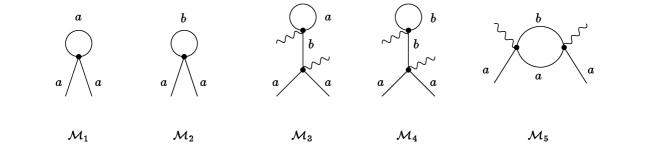
FIG. 7.: Two leg diagrams of order ${\cal O}(\beta_{\kappa})$.

Each of the above diagrams is of ${\cal O}(\beta_{\kappa})$ since each vertex and wavy line contribute ${\cal O}(\beta_{\kappa})$ and ${\cal O}(1/\sqrt{\beta_{\kappa}})$ respectively. The full expression for the ${\cal M}_{i}$ and the calculation of $\rho_{s}$ is given in Appendix B. Writing $\tilde{\rho_{s}}=1/\beta_{A}^{\Delta}-\tilde{\rho_{s}}^{(1)}\tilde{T}$, we have

$$\tilde{\rho_{s}}^{(1)} = \frac{\Gamma(\frac{4-d}{2})}{2^{d+1}\pi^{d/2+2}}\int_{BZ}d^{2}\tilde{k}\left(\epsilon_{+}^{(d-2)/2}+\epsilon_{-}^{(d-2)/2}+\epsilon_{+}^{(d-4)/2}+\frac{\epsilon_{+}^{(d-2)/2}-\epsilon_{-}^{(d-2)/2}}{(d-2)|I(0,0|\tilde{k},-\tilde{k})|}\right).$$ (A1)

For $d\rightarrow 3$, Eq. (A1) can be estimated numerically to give $\mbox{${\tilde{\rho}_{s}}$}^{(1)}\approx 0.295$.

In principle, the one loop correction to $\tilde{c}_{66}$ can be extracted from the propagator Eq. (B17) in a similar manner by setting $q=0$ and expanding in $k$ about $k=0$. However, it is more convenient to start from the definition of the elastic shear modulus. Following Labusch [48], we allow the distortion of the ideal triangular lattice with the constraint that the area of the primitive cell of the first BZ is preserved. $c_{66}$ is then defined as[48]

$$c_{66}=\frac{\eta^{2}}{V}\frac{\partial^{2}F(\eta)}{\partial\eta^{2}}\bigg{\arrowvert}_{\eta_{\Delta}},$$ (A2)

where $\eta$ is a dimensionless variable specifying the shape of the unit cell with area $2\pi\ell^{2}$ (see Appendix D) and $F(\eta)$ is the free energy as a function of $\eta$ as in Eq. (55). However, only the one loop free energy is needed here. The second derivative of $F$ is evaluated at the value of $\eta$ appropriate for a triangular lattice, denoted by $\eta_{\Delta}(=\sqrt{3}/2)$. The mean-field shear modulus has been obtained by Labusch [48], who found $\mbox{$\tilde{c}_{66}$}^{(0)}\approx 0.0885$. By extending this method to one loop order we have:

$$\tilde{c}_{66} = \tilde{c}_{66}^{(0)}+\tilde{c}_{66}^{(1)}{\tilde{T}}$$ (A3)

$$\tilde{c}_{66}^{(1)} = \frac{\eta^{2}\Gamma(\frac{4-d}{2})}{2^{d+1}\pi^{d/2+2}(d-2)}\frac{\partial^{2}\sigma(\eta,d)}{\partial\eta^{2}}\bigg{\arrowvert}_{\eta_{\Delta}},$$ (A4)

where

$$\sigma(\eta,d) = \int_{BZ}d^{2}\tilde{k}\left[\epsilon_{+}^{(d-2)/2}+\epsilon_{-}^{(d-2)/2}\right].$$ (A5)

Our results show that $\sigma(d,\eta)$ has a maximum at $\eta_{\Delta}$ for any $d$ (see Fig. 8). This is consistent with the definition Eq. (A2) where the second derivative is evaluated at a saddle point, i.e. at $\eta_{\Delta}$. However, the total free energy would still have a minimum at $\eta_{\Delta}$ with the curvature of the free energy slightly altered since the mean-field energy $F_{MF}$ dominates for small ${\tilde{T}}$. For $d\rightarrow 3$, we found using the data in Fig. 8 that $\mbox{$\tilde{c}_{66}$}^{(1)}\approx-0.0484$.

Because of the destruction of the Abrikosov lattice at $d=3$, we might have expected that both $\tilde{c}_{66}$ and ${\tilde{\rho}_{s}}$ should be singular. However, at one loop order both of these quantities are found to be finite in the limit $d\rightarrow 3$. The perturbative one loop corrections to $\rho_{s}$ and $c_{66}$ are not ‘aware’ of the destruction of the lattice at $d=3$ in the thermodynamic limit.

However, we believe that in a nonperturbative approach, which would include topological defects such as entanglements, both $c_{66}$ and $\rho_{s}$ would vanish. Notice that in the $(2+\varepsilon)$ treatment of the O(n) model, $n\geq 2$, the mechanism of the transition is the vanishing of the superfluid density, rather than the order parameter[49]. In our case, neither $\rho_{s}$ nor $c_{66}$ is driven to zero by small amplitude thermal fluctuations, and the mechanism of the transition is the vanishing of ODLRO.

FIG. 8.: The function $\sigma/4\pi^{2}$ as a function of $\eta$ for different $d$. The vertical dashed line denotes the position of the peaks at $\eta_{\Delta}$.

B The soft mode propagator and Equation of State

In this appendix, we give the explicit expressions for the one loop diagrams discussed in Appendix A and in Section III. Note that the expressions for ${\cal M}_{5}(p)$ are in abbreviated form, i.e. they are not explicitly even function of the external momentum $p=(k,q)$. Such symmetry must be imposed. The primed parameters $p^{\prime}=(k^{\prime},q^{\prime})$ denotes the internal momentum that has to be integrated over. We shall also use the notation $\int d\vec{p^{\prime}}=\int d^{d-2}q^{\prime}d^{2}k^{\prime}/(2\pi)^{d}$.

$${\cal L}_{2} = \frac{2\beta_{\kappa}\beta_{A}\tilde{\alpha}k_{B}T\sqrt{V}}{\gamma}\int d\vec{p^{\prime}}\left(\frac{\epsilon_{-}(k^{\prime})+1}{\epsilon_{-}(k^{\prime})/\xi_{\parallel}^{2}+q^{\prime 2}}\right)$$ (B1)

$${\cal L}_{3} = \frac{2\beta_{\kappa}\beta_{A}\tilde{\alpha}k_{B}T\sqrt{V}}{\gamma}\int d\vec{p^{\prime}}\left(\frac{\epsilon_{+}(k^{\prime})+1}{\epsilon_{+}(k^{\prime})/\xi_{\parallel}^{2}+q^{\prime 2}}\right)$$ (B2)

$${\cal M}_{1}(p) = \frac{-2\beta_{\kappa}\beta_{A}}{k_{B}T}\int d\vec{p^{\prime}}G_{a}(p^{\prime})\left(I(k^{\prime},k|k^{\prime},k)+2Re\left[Q_{k^{\prime}}^{2}Q_{k}^{*2}I(k,-k|k^{\prime},-k^{\prime})\right]\right)$$ (B3)

$${\cal M}_{2}(p) = \frac{-2\beta_{\kappa}\beta_{A}}{k_{B}T}\int d\vec{p^{\prime}}G_{b}(p^{\prime})\left(I(k^{\prime},k|k^{\prime},k)-2Re\left[Q_{k^{\prime}}^{2}Q_{k}^{*2}I(k,-k|k^{\prime},-k^{\prime})\right]\right)$$ (B4)

$${\cal M}_{3}(p) = \frac{\beta_{\kappa}\beta_{A}}{k_{B}T}\int d\vec{p^{\prime}}G_{a}(p^{\prime})\bigg{[}\epsilon_{-}(k^{\prime})+1\bigg{]}\bigg{[}\epsilon_{-}(k)+1\bigg{]}$$ (B5)

$${\cal M}_{4}(p) = \frac{\beta_{\kappa}\beta_{A}}{k_{B}T}\int d\vec{p^{\prime}}G_{b}(p^{\prime})\bigg{[}\epsilon_{+}(k^{\prime})+1\bigg{]}\bigg{[}\epsilon_{-}(k)+1\bigg{]}$$ (B6)

$${\cal M}_{5}(p) = \frac{4\beta_{\kappa}|\alpha_{H}|\beta_{A}}{(k_{B}T)^{2}}\int d\vec{p^{\prime}}G_{a}(p^{\prime}-p)G_{b}(p^{\prime})\times$$ (B17)

$$\Big{\{}\left|I(0,k^{\prime}|k,k^{\prime}-k)\right|^{2}+|I(0,k|k^{\prime},k-k^{\prime})|^{2}+|I(0,k-k^{\prime}|k,-k^{\prime})|^{2}$$

$$~{}~{}~{}~{}~{}+4Re\left[Q_{k^{\prime}}^{2}I(0,k|k^{\prime},k-k^{\prime})I(0,k-k^{\prime}|k,-k^{\prime})\right]$$

$$~{}~{}~{}~{}~{}-4Re\left[Q_{k}^{2}I(0,k^{\prime}|k^{\prime}-k,k)I(0,k^{\prime}-k|k^{\prime},-k)\right]$$

$$~{}~{}~{}~{}~{}-4Re\left[Q_{k-k^{\prime}}^{2}I(0,k^{\prime}|k^{\prime}-k,k)I(0,k|k-k^{\prime},k^{\prime})\right]$$

$$~{}~{}~{}~{}~{}+8Re\left[Q_{k^{\prime}}^{*2}Q_{k}^{2}Q_{k^{\prime}-k}^{2}I^{2}(0,k^{\prime}|k,k^{\prime}-k)\right]$$

$$~{}~{}~{}~{}~{}+8Re\left[Q_{k^{\prime}}^{2}Q_{k}^{*2}Q_{k-k^{\prime}}^{2}I^{2}(0,k|k^{\prime},k-k^{\prime})\right]$$

$$~{}~{}~{}~{}~{}+8Re\left[Q_{k^{\prime}}^{2}Q_{k}^{2}Q_{k^{\prime}-k}^{*2}I^{2}(0,k^{\prime}-k|k^{\prime},-k)\right]$$

$$~{}~{}~{}~{}~{}+8Re\left[Q_{k}^{2}Q_{k^{\prime}-k}^{*2}I(0,k-k^{\prime}|k,-k^{\prime})I(k-k^{\prime},k^{\prime}|0,k)\right]$$

$$~{}~{}~{}~{}~{}-8Re\left[Q_{k^{\prime}}^{*2}Q_{k}^{2}I(0,k^{\prime}|k^{\prime}-k,k)I(k-k^{\prime},k^{\prime}|0,k)\right]$$

$$~{}~{}~{}~{}~{}-8Re\left[Q_{k^{\prime}}^{*2}Q_{k^{\prime}-k}^{2}I(0,k^{\prime}|k,k^{\prime}-k)I(k,-k^{\prime}|0,k-k^{\prime})\right]\Big{\}}.\vspace{0.5cm}$$

The renormalized soft mode propagator to one-loop order is such that

$$\tilde{G}^{-1}_{a}(p)=G_{a}^{-1}(p)+{\cal M}_{1}(p)+{\cal M}_{2}(p)+{\cal M}_{3}(p)+{\cal M}_{4}(p)+{\cal M}_{5}(p).$$ (B18)

The propagator $\tilde{G}_{a}(k)$ is still massless. This can easily shown by setting the external momentum $p=0$. Indeed, $\tilde{G}_{a}$ is expected to be massless to all orders in the loop expansion [33]. The superfluid density [50] can be calculated using the following relation for small $q$:

$$\rho_{s}q^{2}=2k_{B}T\tilde{G}^{-1}_{a}(q,k=0)\tilde{\alpha}^{2}.$$ (B19)

Substituting Eq. (38) into Eq. (B18), we have:

$$\frac{\rho_{s}}{\alpha_{0}^{2}} = \gamma-\frac{\beta_{\kappa}\beta_{A}k_{B}T}{|\alpha_{H}|}\int d\vec{p^{\prime}}\times\Bigg{\{}\frac{\epsilon_{+}(k^{\prime})+2}{\epsilon_{+}(k^{\prime})/\xi_{\parallel}^{2}+q^{\prime 2}}+\frac{4|\alpha_{H}||I(0,0|k^{\prime},-k^{\prime})|}{\gamma(\epsilon_{+}(k^{\prime})/\xi_{\parallel}^{2}+q^{\prime 2})^{2}}$$ (B21)

$$~{}~{}~{}~{}~{}~{}~{}~{}~{}~{}~{}~{}~{}~{}+\frac{\epsilon_{-}(k^{\prime})}{\epsilon_{-}(k^{\prime})/\xi_{\parallel}^{2}+q^{\prime 2}}+\frac{32|\alpha_{H}|^{2}q^{\prime 2}|I(0,0|k^{\prime},-k^{\prime})|^{2}}{\gamma^{2}(d-2)(\epsilon_{-}(k^{\prime})/\xi_{\parallel}^{2}+q^{\prime 2})(\epsilon_{+}(k^{\prime})/\xi_{\parallel}^{2}+q^{\prime 2})^{3}}\Bigg{\}}.$$

All integrals in Eq. (B21) are infrared convergent. On integrating over $q^{\prime}$, Eq. (B21) yields Eq. (A1). Similarly, one can calculate $c_{66}$ in principle via

$$c_{66}\ell^{4}k^{4}=2k_{B}T\tilde{G}^{-1}_{a}(k\rightarrow 0,q=0)\tilde{\alpha}^{2}.$$ (B22)

However, expressing ${\cal M}_{i}$ in terms of explicit polynomial of small $k$ is a challenging task. One would expected that the leading order should be $k^{4}$ corresponding to a dispersion appropriate to the elastic shear mode. A more straightforward way of calculating the correction to $c_{66}$ is to use the definition discussed in Appendix A.

C Loop expansion of the free energy

As discussed in Section IV, the starting point of our calculation of the jumps in the magnetization and the entropy is the 3D free energy. In this appendix, we derive the 3D free energy expansion about the mean-field solution to two loop order starting from the definition:

$$F=-k_{B}T\ln\left(\prod_{p}\int[{\cal D}a_{p}][{\cal D}b_{p}]\exp(-{\cal F}/k_{B}T)\right).$$ (C1)

At the one loop level, we substitute the Gaussian functional Eq. (18) into Eq. (C1), and we obtain the correction to the mean-field as:

$$F^{(1)} = \frac{k_{B}T}{2}\sum_{k,q}\left[\ln\left(\frac{2|\alpha_{H}|\epsilon_{+}(k)+\gamma q^{2}}{2\pi k_{B}T}\right)+\ln\left(\frac{2|\alpha_{H}|\epsilon_{-}(k)+\gamma q^{2}}{2\pi k_{B}T}\right)\right]$$ (C2)

$$= \frac{|\alpha_{H}|^{2}V}{2\beta_{\kappa}\beta_{A}}\left[\frac{\beta_{A}{\tilde{T}}}{4\pi^{3}}\int d^{2}\tilde{k}(\epsilon_{+}(\tilde{k})^{(d-2)/2}+\epsilon_{-}(\tilde{k})^{(d-2)/2})\right]+k_{B}T\sum_{k,q}\left[\ln\left(\frac{\gamma q^{2}}{2\pi k_{B}T}\right)\right].$$ (C3)

The first and second term in Eq. (C3) correspond to $F^{(1)}-F^{(1)}(\alpha_{H}=0)$ and $F^{(1)}(\alpha_{H}=0)$ respectively. The second term is dependent on an ultraviolet cutoff in the longitudinal vector $q$. The cutoff is of the order of the reciprocal of the layer spacing of the model. Since we are interested in the long wavelength limit, we follow the standard prescription of absorbing this term into the normal phase energy (see Ref. [37]). Using this results in Eq. (55), with ${\cal E}^{(1)}\approx 0.524$ for $d=3$.

For the sake of simplicity, we set $d=3$ at the outset when discussing the two loop calculation. The total two loop free energy can be written as

$${\cal E}^{(2)}=\frac{\beta_{A}^{2}}{8\pi^{2}}({\cal E}_{s}+{\cal E}_{h}).$$ (C4)

${\cal E}_{s}$ is the sum of energy diagrams involving the soft mode and ${\cal E}_{h}$ is the sum of diagrams containing the hard mode only. After integrating over the longitudinal component $q$, and expressing the remaining transverse integral in terms of the dimensionless BZ (to simplify notation, the tilde on $k$ and $k^{\prime}$ are dropped), we have

$${\cal E}_{s} = \sum_{i=1}^{5}{\cal E}_{i}$$ (C5)

$${\cal E}_{1} = \int\int\frac{d^{2}kd^{2}k^{\prime}}{(4\pi^{2})^{2}}\frac{-f_{+}(k,k^{\prime})}{\sqrt{\epsilon_{-}(k)\epsilon_{-}(k^{\prime})}}$$ (C6)

$${\cal E}_{2} = \int\int\frac{d^{2}kd^{2}k^{\prime}}{(4\pi^{2})^{2}}\frac{-2f_{-}(k,k^{\prime})}{\sqrt{\epsilon_{-}(k)\epsilon_{+}(k^{\prime})}}$$ (C7)

$${\cal E}_{3} = \int\int\frac{d^{2}kd^{2}k^{\prime}}{(4\pi^{2})^{2}}\frac{(\epsilon_{-}(k^{\prime})+1)(\epsilon_{-}(k)+1)}{2\sqrt{\epsilon_{-}(k)\epsilon_{-}(k^{\prime})}}$$ (C8)

$${\cal E}_{4} = \int\int\frac{d^{2}kd^{2}k^{\prime}}{(4\pi^{2})^{2}}\frac{(\epsilon_{+}(k^{\prime})+1)(\epsilon_{-}(k)+1)}{\sqrt{\epsilon_{+}(k^{\prime})\epsilon_{-}(k)}}$$ (C9)

$${\cal E}_{5} = \int\int\frac{d^{2}kd^{2}k^{\prime}}{(4\pi^{2})^{2}}\frac{g(k,k^{\prime})}{\sqrt{\epsilon_{+}(k+k^{\prime})\epsilon_{-}(k)\epsilon_{-}(k^{\prime})}(\sqrt{\epsilon_{+}(k+k^{\prime})}+\sqrt{\epsilon_{-}(k)}+\sqrt{\epsilon_{-}(k^{\prime}})},$$ (C10)

where

$$f_{\pm}(k,k^{\prime}) = I(k,k^{\prime}|k,k^{\prime})\pm 2Re\left[Q_{k^{\prime}}^{*2}Q_{k}^{2}I(k,-k|k^{\prime},-k^{\prime})\right]$$ (C11)

$$g(k,k^{\prime}) = 16[Re(Q_{k-k^{\prime}}^{*}Q_{k^{\prime}}Q_{k}I(0,k^{\prime}-k|k^{\prime},-k))]^{2}$$ (C12)

$$+ 16\{Re[Q^{*}_{k}Q_{k^{\prime}}Q_{k-k^{\prime}}I(0,k|k^{\prime},k-k^{\prime})+Q^{*}_{k^{\prime}}Q_{k}Q_{k-k^{\prime}}I(0,k^{\prime}|k,k^{\prime}-k)]\}^{2}$$ (C13)

$$- 32Re\{Q_{k-k^{\prime}}^{*}Q_{k}Q_{k^{\prime}}I(0,k-k^{\prime}|-k^{\prime},k)\}Re\{Q_{k}Q_{k^{\prime}}Q_{k^{\prime}-k}I(0,k|k^{\prime},k-k^{\prime})\}$$ (C14)

$$- 32Re\{Q_{k-k^{\prime}}^{*}Q_{k}Q_{k^{\prime}}I(0,k-k^{\prime}|-k^{\prime},k)\}Re\{Q_{k^{\prime}}Q_{k}Q_{k^{\prime}-k}I(0,k^{\prime}|k,k^{\prime}-k)\}.$$ (C15)

Each integral involving $1/\sqrt{\epsilon_{-}}$ is logarithmically divergent in the infrared-limit, but the sum of the integrands of ${\cal E}_{i}$ is finite in the infra-red limit ($k^{\prime},k\rightarrow 0$), and hence ${\cal E}_{s}$ is finite. Numerically, we find that ${\cal E}_{s}\approx 0.8$. The diagrams in ${\cal E}_{h}$ are given by the expressions:

$${\cal E}_{h} = \sum_{i=6}^{8}{\cal E}_{i}$$ (C16)

$${\cal E}_{6} = \int\int\frac{d^{2}kd^{2}k^{\prime}}{(4\pi^{2})^{2}}\frac{-f_{+}(k^{\prime},k)}{\sqrt{\epsilon_{+}(k)\epsilon_{+}(k^{\prime})}}\approx-0.89$$ (C17)

$${\cal E}_{7} = \frac{1}{2}\left[\int\frac{d^{2}k}{4\pi^{2}}\left(\frac{1}{\sqrt{\epsilon_{+}(k)}}+\sqrt{\epsilon_{+}(k)}\right)\right]^{2}\approx 2.07$$ (C18)

$${\cal E}_{8} = \int\int\frac{d^{2}kd^{2}k^{\prime}}{(4\pi^{2})^{2}}\frac{h(k,k^{\prime})}{\sqrt{\epsilon_{+}(k^{\prime}+k)\epsilon_{+}(k^{\prime})\epsilon_{+}(k)}[\sqrt{\epsilon_{+}(k+k^{\prime})}+\sqrt{\epsilon_{+}(k^{\prime})}+\sqrt{\epsilon_{+}(k)}]}\approx 0.62,$$ (C19)

where

$$h(k,k^{\prime}) = ~{}4Re[Q_{k+k^{\prime}}^{2}I(0,k^{\prime}|-k,k+k^{\prime})I(0,k|-k^{\prime},k+k^{\prime})]$$ (C22)

$$+8Re[Q_{k}^{*2}Q_{k^{\prime}}^{2}I(0,k|-k^{\prime},k+k^{\prime})I(-k,k^{\prime}+k|0,k^{\prime})]$$

$$+16\left[Re(Q_{k^{\prime}}^{*}Q_{k}Q_{k+k^{\prime}}I(0,k^{\prime}|-k,k+k^{\prime}))\right]^{2}.$$

All integrals can be evaluated numerically, and we found that ${\cal E}_{h}\approx 1.80$.

D The first BZ and the Function $I(k_{1},k_{2}\mid k_{3},k_{4})$

In this appendix, we briefly outline a procedure for evaluating integrals involving $I(k_{1},k_{2}\mid k_{3},k_{4})$ over the first BZ. Intgerals over the longitudinal vector $q$ can be done analytically, but the integration over $k$ in the first BZ is done numerically.

Restricting ourselves to the class of centered rectangular lattices[51], the fundamental unit cell of the vortex lattice can be characterized by two primitive vectors ${\bf r}_{\rm I}=(1,0)\ell_{0}$ and ${\bf r}_{\rm II}=(1/2,\eta)\ell_{0}$, where $\ell_{0}$ is the spacing between vortices. The flux quantization condition determines the area of the unit cell as $2\pi\ell^{2}(=\eta\ell_{0}^{2})$. The corresponding first BZ has an area of $4\pi^{2}/\eta\ell_{0}^{2}$. It is convenient to rescale the transverse length by $\sqrt{2\pi}\ell$, and construct a dimensionless unit cell with primitive vectors ${\bf r}^{\prime}_{\rm I}=(1/\sqrt{\eta},0)$ and ${\bf r}^{\prime}_{\rm II}=(1/2\sqrt{\eta},\sqrt{\eta})$, giving an area of unity. A dimensionless vector $\tilde{k}$ can be defined as $\sqrt{2\pi}\ell k$. The corresponding dimensionless BZ in the reciprocal lattice has area $4\pi^{2}$. By changing $\eta$, one can construct a unit cell of different shape with the area remaining unchanged. The ideal triangular and square lattices correspond to $\eta_{\Delta}=\sqrt{3}/2$, and $\eta_{\Box}=1/2$ respectively. In this paper, all the integrals are evaluated at $\eta_{\Delta}$ except in the calculation of $c_{66}$ in Eq. (A2).

In general, the function $I(\tilde{k}_{1},\tilde{k}_{2}|\tilde{k}_{3},\tilde{k}_{4})$ can be expressed in terms of gauge invariant reciprocal lattice sums [52, 53]. To simplify notation, we will ignore the tilde assigned to the dimensionless $k$ vector and exploit the conservation of momentum ${\bf k}_{1}+{\bf k}_{2}={\bf k}_{3}+{\bf k}_{4}$ on each quartic vertex.

$$I(k_{1},k_{2}|k_{3},k_{4}) = \exp\left[-|{\bf k}_{2}-{\bf k}_{4}|^{2}/4\pi-i(k_{y2}-k_{y4})(k_{x2}-k_{x3})/2\pi\right]$$ (D3)

$$\sum_{m,n}\Theta_{m,n}\exp\left[-(k_{y2}+ik_{x2})(ig_{x}-g_{y})\right]$$

$$\times\exp\left[-(g_{y}k_{y4}+g_{x}k_{x4})+i(g_{x}k_{y3}-g_{y}k_{x3})\right],$$

where $(g_{x},g_{y})=(m\sqrt{\eta},(n-m/2)/\sqrt{\eta})$ are dimensionless reciprocal lattice vectors, and $\Theta_{m,n}=\exp[-\pi(g_{x}^{2}+g_{y}^{2})]/\beta_{A}$. In particular,

$$I(0,0|0,0) = \sum_{m,n}\Theta_{m,n}=1$$ (D4)

$$I(0,k|0,k) = \sum_{m,n}\Theta_{m,n}\exp\left[i\bigg{[}k_{y}g_{x}-k_{x}g_{y}\bigg{]}\right]$$ (D5)

$$\approx 1-\left(\frac{\eta}{4\pi\surd{3}}\right)k^{2}+0.0029k^{4}+\cdots,~{}~{}~{}~{}~{}~{}~{}~{}~{}~{}k\rightarrow 0$$ (D6)

$$|I(0,0|k,-k)| = \bigg{|}\sum_{m,n}\Theta_{m,n}\exp\left[\bigg{(}k_{y}-ik_{x}\bigg{)}\left(ig_{x}+g_{y}\right)-\frac{k^{2}}{4\pi}\right]\bigg{|}$$ (D7)

$$\approx 1-\left(\frac{\eta}{2\pi\surd{3}}\right)k^{2}+0.0032k^{4}+\cdots,~{}~{}~{}~{}~{}~{}~{}~{}~{}~{}k\rightarrow 0.$$ (D8)

Within the BZ, it can be shown that $0<\epsilon_{-}<0.59<\epsilon_{+}<1$. The asymptotic behavior of $\epsilon_{\pm}$ can be shown to be at small $k$:

$$\epsilon_{+}(k) \approx 2-\left(\frac{\eta}{\pi\surd{3}}\right)k^{2}+0.0099k^{4}+\cdots$$ (D9)

$$\epsilon_{-}(k) \approx \frac{\tilde{c}_{66}\beta_{A}}{(2\pi)^{2}}k^{4}=0.0026k^{4}+\cdots.$$ (D10)

It is instructive to plot the contour of the function $\epsilon_{\pm}(\tilde{k})$ for a triangular lattice configuration to illustrate its symmetries and the first BZ (see Fig. 9). The maxima and minima are denoted by the light and dark shades respectively. The reciprocal lattice vector(RLV) points are marked either by the maxima of $\epsilon_{+}$ or the minima of $\epsilon_{-}$. The equal-sided hexagonal BZ can be constructed by joining together the six minima (maxima) surrounding the central RLV in the function $\epsilon_{+}$ ($\epsilon_{-}$). It is easy to see that approximating the two dimensional integration by a circular BZ underestimates the integrand involving $\epsilon_{-}(\tilde{k})$ as the function has spikes at the corners of the Brillouin zone.

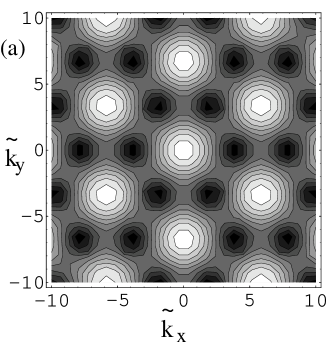
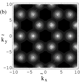
FIG. 9.: The contour plot of the functions (a)$\epsilon_{+}(\tilde{k})$ and (b)$\epsilon_{-}(\tilde{k})$ for the triangular configuration.

REFERENCES

• [1]  A. A. Abrikosov, Zh. Eksp. Teor. Fiz. [Sov. Phys. JETP] 5, 1174 (1957).
• [2] R. Liang, D. A. Bonn, and W. N. Hardy, Phys. Rev. Lett. 76, 1996 (1996).
• [3] U. Welp et al., Phys. Rev. Lett. 76, 4809 (1996).
• [4] E. Zeldov et al., Nature 375, 373 (1995).
• [5] A. Schilling et al., Nature 382, 791 (1996).
• [6] A. Junod et al., Physica C 275, 384 (1997).
• [7] R. E. Hetzel, A. Sudbø, and D. A. Huse, Phys. Rev. Lett. 69, 518 (1992).
• [8] T. Chen and S. Teitel, Phys. Rev. B 55, 11766 (1997); Phys. Rev. B 55, 15197 (1997).
• [9] A. K. Nguyen and A. Sudbø, preprint cond-mat/9705223.
• [10] R. Šášik and D. Stroud, Phys. Rev. Lett. 75, 2582 (1995).
• [11] J. Hu and A. H. MacDonald, Phys. Rev. B 56, 2788 (1997).
• [12] M. J. W. Dodgson and M. A. Moore, Phys. Rev. B 55, 3816 (1997).
• [13] R. Šášik and D. Stroud, Phys. Rev. B 48, 9938 (1993).
• [14] R. Šášik and D. Stroud,  Phy. Rev. Lett. 72, 2462 (1994); Phys. Rev. B, 49 16074 (1994).
• [15] Z. Tešanović and L. Xing, Phys. Rev. Lett. 67, 2729 (1991).
• [16] Y. Kato and N. Nagaosa,  Phys. Rev. B, 47, 2932 (1993); Phys. Rev. B, 48, 7383 (1993).
• [17] J. Hu and A. H. MacDonald, Phys. Rev. Lett. 71, 432 (1993).
• [18] J. A. O’Neill and M. A. Moore, Phys. Rev. B 48, 374 (1993).
• [19] E. Brézin, D. R. Nelson, and A. Thiaville, Phys. Rev. B 31, 7124 (1985).
• [20] G. Blatter et al., Rev. Mod. Phys. 66, 1125 (1994).
• [21] L. L. Daemen, L. N. Bulaevskii, M. P. Maley, and J. Y. Coulter,  Phys. Rev. Lett. 70, 1167 (1993); Phys. Rev. B 47, 11291 (1993).
• [22] R. Cubitt et al., Nature 365, 407 (1993).
• [23] K. Maki and H. Takayama, Prog. Theor. Phys. 46, 1651 (1971).
• [24] M. A. Moore, Phys. Rev. B 39, 136 (1989).
• [25] M. A. Moore, Phys. Rev. B 45, 7336 (1992).
• [26] M. A. Moore, Phys. Rev. B 55, 14136 (1997).
• [27] This 3D to 2D crossover is purely a finite size effect and should not be confused with the decoupling mechanism of the vortices mentioned earlier.
• [28] D. López, E. F. Righi, G. Nieva, and F. de la Cruz, Phys. Rev. Lett. 76, 4034 (1996).
• [29] A. K. Kienappel and M. A. Moore, in preparation. Preliminary results from the Monte Carlo simulations on a sphere using the LLL approximation also suggest exponential growth of $\ell_{\parallel}$. However, determination of A from simulations is difficult as a very large number of vortices are needed to enable the system to be in the asymptotic regime discussed in this paper.
• [30] A. Schilling et al., Phys. Rev. Lett. 78, 4833 (1997).
• [31] G. Eilenberger, Phys. Rev. 164, 628 (1967).
• [32] S.-K. Ma, Modern Theory of Critical Phenomena (W.A. Benjamin, Reading, Mass., 1976).
• [33] D. J. Wallace, in Phase Transition and Critical Phenomena, edited by C. Domb and M. S. Green (Academic Press Inc., London, 1976), Vol. 6.
• [34] G. J. Ruggeri, Phys. Rev. B 20, 3626 (1979).
• [35] S. L. Lee et al., Phys. Rev. Lett 75, 922 (1995).
• [36] J. Yeo and M. A. Moore, Phys. Rev. Lett 78, 4490 (1997).
• [37] G. J. Ruggeri and D. J. Thouless, J. Phys. F: Metal Phys. 6, 2063 (1976).
• [38] N. K. Wilkin and M. A. Moore, Phys. Rev. B 48, 3464 (1993).
• [39] S. Hikami, A. Fujita, and A. I. Larkin, Phys. Rev. B 44, 10400 (1991).
• [40] The mean field coherence length $\xi^{MF}_{\perp}(0)$ is approximately the same in YBCO and BSCCO, and therefore $B_{c2}(0)\approx\Phi_{0}/2\pi\xi^{MF}_{\perp}(0)^{2}$ are also approximately the same in both cases. We have used a typical value of $B_{c2}(0)\approx 170T$ which coressponds to $\xi_{\perp}^{MF}(0)\approx 14\AA$.
• [41] G. Blatter, V. B. Geshkenbein, and A. I. Larkin, Phys. Rev. Lett. 68, 875 (1992).
• [42] M. Roulin, A. Junod, and E. Walker, Science 273, 1210 (1996).
• [43] A. K. Kienappel and M. A. Moore, to appear in Phys. Rev. B.
• [44] T. Nishizaki et al., Phys. Rev. B 53, 82 (1996).
• [45] H. Safar et al., Phys. Rev. Lett. 70, 3800 (1993).
• [46] J. A. Fendrich et al., Phys. Rev. Lett. 74, 1210 (199).
• [47] A. I. Larkin, Zh. Eksp. Teor. Fiz. [Sov. Phys. JETP] 58, 1466 (1970).
• [48] R. Labusch, Phys. Status Solidi 32, 439 (1969).
• [49] J. J. Binney, N. J. Dowrick, A. J. Fisher, and M. E. J. Newman, The Theory of Critical Phenomena: An Introduction to the Renormalization Group (Clarendon Press, Oxford, 1992).
• [50] P. C. Hohenberg and P. C. Martin, Annals of Physics 34, 291 (1965).
• [51] W. H. Kleiner, L. M. Roth, and S. H. Autler, Phys. Rev. 133, 1226 (1964).
• [52] E. H. Brandt, Phys. Stat. Sol. 36, 381 (1969).
• [53] J. Yeo, private communication.