[

Errors in Hellmann-Feynman Forces due to occupation number broadening, and how they can be corrected

Abstract

In ab initio calculations of electronic structures, total energies, and forces, it is convenient and often even necessary to employ a broadening of the occupation numbers. If done carefully, this improves the accuracy of the calculated electron densities and total energies and stabilizes the convergence of the iterative approach towards self-consistency. However, such a boardening may lead to an error in the calculation of the forces. Accurate forces are needed for an efficient geometry optimization of polyatomic systems and for ab initio molecular dynamics (MD) calculations. The relevance of this error and possible ways to correct it will be discussed in this paper. The first approach is computationally very simple and in fact exact for small MD time steps. This is demonstrated for the example of the vibration of a carbon dimer and for the relaxation of the top layer of the (111)-surfaces of aluminium and platinum. The second, more general, scheme employs linear-response theory and is applied to the calculation of the surface relaxation of Al (111). We will show that the quadratic dependence of the forces on the broadening width enables an efficient extrapolation to the correct result. Finally the results of these correction methods will be compared to the forces obtained by using the smearing scheme, which has been proposed by Methfessel and Paxton.

]

In ab initio electronic structure and total energy calculations the integrals over the Brillouin zone are commonly replaced by the sum over a mesh of k-points[1, 2]. This approach is very efficient for insulators, but for metallic systems convergence with respect to the number of k-points becomes slow. Here the introduction of fractional occupation numbers is a convenient way to improve the k-space integration and in addition to stabilize the convergence in the iterative approach to self-consistency. In these broadening schemes the eigenstates are occupied according to a smooth function, e.g. a Gaussian [3] or the Fermi function [4, 5, 7, 8] at a finite temperature.

When a broadening scheme is employed in a density functional theory calculation, the computed electron density of the ground state $n_{0}({\bf r})$ does not minimize the functional of the total energy $E$ but the functional of the free energy $A$:

$$A\left[T_{\text{el}};n\right]=E\left[T_{\text{el}};n\right]-T_{\text{el}}S\left[T_{\text{el}};n\right]\quad,$$ (1)

where $S$ denotes the entropy associated with the occupation numbers of the Kohn-Sham orbitals and $T_{\rm el}$ is the broadening parameter. In the case of Fermi broadening[6] we get:

$$S=-k_{B}\sum_{i}\left[f_{i}\ln f_{i}+\left(1-f_{i}\right)\ln\left(1-f_{i}\right)\right]\quad.$$ (2)

Since the temperatures commonly used for the broadening are much higher than the physical ones (it is convinient to use $k_{B}T_{\text{el}}\sim 0.1~{}\text{eV}$), neither the total energies nor the free energies (Eq. 1) are directly meaningful.

One way to obtain the ground state energy at zero temperature is based on the well known fact[6], that for the free electron gas, the quantities $A$ and $E$ depend quadratically on $T_{\text{el}}$. Therefore one can write:

$$A\left(T_{\text{el}}\right)=E^{\text{zero}}-\frac{1}{2}\gamma^{2}T_{\text{el}}^{2}+O\left(T_{\text{el}}^{3}\right)\quad$$ (3)

$$E\left(T_{\text{el}}\right)=E^{\text{zero}}+\frac{1}{2}\gamma^{2}T_{\text{el}}^{2}+O\left(T_{\text{el}}^{3}\right)\quad.$$ (4)

As it was pointed out by Gillan[7], it follows from Eqs. (1), (3) and (4) that the extrapolation of the total energy towards the $T_{\text{el}}$=0 result is:

$$E^{\text{zero}} = E(T_{\text{el}}\rightarrow 0)=A(T_{\text{el}}\rightarrow 0)$$ (5)

$$\approx E(T_{\text{el}})-\frac{1}{2}T_{\text{el}}S(T_{\text{el}})\quad.$$ (6)

Obtaining $E^{\text{zero}}$ using Eqs. (6) and (2) is straightforward and gives very satisfactory results[8]. This is shown in Figure 1(a) for a slab consisting of four layers of Aluminium. Here the extrapolation (filled circles) matches perfectly the zero-temperature energy, even for quite large broadening temperatures. For a systems like Platinum, which was chosen as an example for a not free electron like system, Figure 1(b) shows, that this extrapolation is indeed an approximation. But if the broadening parameter is chosen carefully (typically used broadenig parameters are about 0.1 eV or lower) the extrapolation still gives acceptable results.

Calculating the forces, however, is more complicated. The forces on atoms are defined as the derivative of the total energy $E^{\text{zero}}$ with respect to the atomic positions:

$${\bf F}^{\text{zero}} = -\frac{\partial E^{\text{zero}}}{\partial{\bf R}}$$ (7)

$${\bf F}^{\text{zero}} = -\frac{\partial A}{\partial{\bf R}}-\frac{1}{2}T_{\text{el}}\frac{\partial S}{\partial{\bf R}}$$ (8)

FIG. 1.: Total energy $E(k_{\rm B}T_{\rm el})$ (open diamonds, dash-dotted line) and energy extrapolated to $k_{\rm B}T_{\rm el}=0\>{\rm eV}$ $E^{\rm zero}$ (filled circles, solid line) as a function of $k_{\rm B}T$ using a Fermi broadening and total energy $E^{\rm tot}$ (open squares, dashed line) using the Methfessel-Paxon smearing of first order for a slab of four-layers of aluminuim (a) and platinum (b). Dots present computed values, lines are fits to guide the eye.

While the quantity

$${\bf F}^{\rm HF}(T_{\text{el}})=-\frac{\partial A}{\partial{\bf R}}$$ (9)

is easily evaluated, the evaluation of $\partial S/\partial{\bf R}$ is somewhat more elaborate. Neglecting the entropy term in Eq. (8) implies that the forces are not in agreement with the gradient of the total energy of Eq. (6). As a consequence, when those forces are used to relax the atoms towards their equilibrium positions, the obtained geometry is likely to be different from that which minimizes $E^{\text{zero}}$. Figure 2 presents results for a four-layers aluminum (111) slab, with fully separable, norm-conserving pseudopotentials[9, 10], a plane-wave basis set ($E^{\text{cut}}=8~{}\text{Ry}$) and 18 $\bf k$-points[11] to sample the surface Brillouin zone. An untipically high broadening of $0.5~{}\text{eV}$ was used to show the effect and it is clearly visible that the Hellmann-Feynmann-Force ${\bf F}^{\rm HF}(T_{\text{el}})$ acting on the surface layer vanishes for the position minimizing the free energy, as it should according to Eq. (9). But the minimum of the total energy is at a different position.
Even at this untypically high broadening temperature, which was chosen to illustrate the effect, the error in the equilibrium position is only $10^{-3}$ nm, which is less than one percent of the interlayer distance. This indicates, that the error in the forces due to occupation number

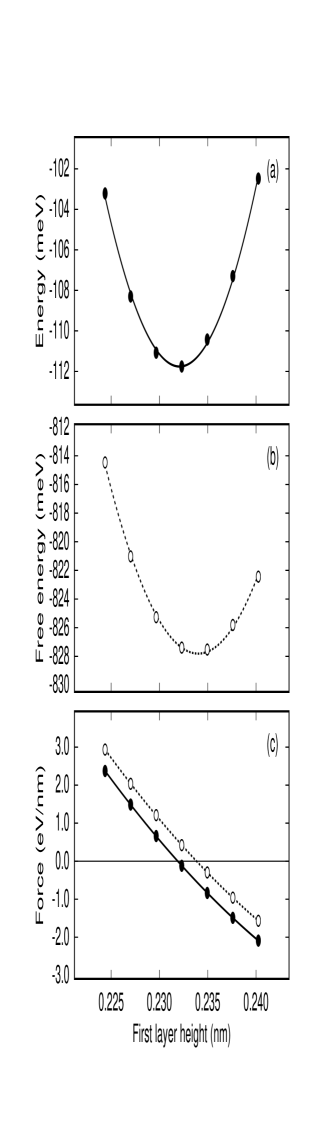
FIG. 2.: (a) Zero-temperature energy $E^{\text{zero}}$ and (b) free energy $A$ of a four-layers Al (111) slab as a function of the height $Z$ of the first atomic layer. To demonstrate the effect, a Fermi-Dirac broadening with an untypically high broadening pararmeter $k_{B}T_{\text{el}}$=0.5 eV has been used. (c) Force acting on the first atomic layer (open dots are non-corrected and full dots are corrected forces). Dots present computed values, lines are fits to guide the eye.

broadening may be neglegible in the case of relaxations if the temperature is chosen not unreasonable high, but unfortunally this has to be checked for each particular system.

The situation is less clear and the needs are more demanding, when it comes to molecular dynamics (MD) simulations. When the non-corrected forces (Eq. 9) are used to perform MD, the sum of potential kinetic energies of the atoms is not a conserved quantity. An illustration of this is shown in Figure 3(a) for a MD simulation of the vibration of a carbon dimer. The graph shows the total energy (open circles) and the free energy (closed circles) of the systems as a function of the interatomic distance. The trajectory was integrated over approx. two periods using the verlet algorithm and no thermostat had been employed. Using the non-corrected forces produces a motion in which the total energy is not conserved but oscillates with the frequency of the motion. Figure 3(a) cleary shows, that at the turning points, where the kinetic energy vanishes, the potential energies are different, which is obviously unphysical. In fact, the free energies, given by Eq. (1), at the turning points are equal.

Plotting the eigenvalues as a function of the intermolecular distance (Fig. 4(b)) shows a crossing of the $2\sigma_{g}$ level and the two-fold degenerated $1\pi_{u}$ levels near

FIG. 3.: Free Energy $E^{\text{zero}}$ (filled circles) and total energy $E$ (open circles) as a function of interatomic distance during the vibration of a carbon dimer. The points are taken at different times during the vibration. The border points at the outer left and right are the turning points of the motion, thus the range of distances covered in each figure correspond to the amplitude of the vibration. (a) Non-corrected forces have been used for the molecular dynamics. Obviously the potential energy at the two turning points is very different. (b) Corrected forces have been used for the molecular dynamics. The potential energy at the two turning points is nearly the same.

the equilibrium distance $d_{0}$. Since in the groundstate, the $2\sigma_{g}$ level is empty (LUMO), while the $1\pi_{u}$ levels are fully occupied (HOMO), the introduction of a broadening function causes a noticeable change in the occupation numbers of these orbitals (Fig. 4(a)) during the vibration. This leads to a non-negligible correction to ${\bf F}(T_{\text{el}})$ according to Eq. 8. We will now describe how this entropy contribution to the forces can be evaluated. From Eq. (2), one obtains the expression for $T_{\text{el}}\partial S/\partial{\bf R}$:

$$T_{\text{el}}\frac{\partial S}{\partial{\bf R}}=-2k_{B}T_{\text{el}}\sum_{i}\frac{\partial f_{i}}{\partial{\bf R}}\ln\frac{f_{i}}{1-f_{i}}\quad,$$ (10)

which, in the case of a Fermi distribution for the occupation numbers, reduces to

$$T_{\text{el}}\frac{\partial S}{\partial{\bf R}}=2\sum_{i}\frac{\partial f_{i}}{\partial{\bf R}}\epsilon_{i}\quad.$$ (11)

The $\epsilon_{i}$ denote the energies of the Kohn-Sham orbitals. Using a Fermi distribution for the $f_{i}$, we find, that in the case of the vibrating dimer on the relevant length scales the occupation numbers change linearly with R (see Fig. 4(a)), i.e. $\partial f_{i}/\partial{\bf R}$ is nearly a constant. Figure 3(b) illustrates the symmetric and total energy-conserving vibrations obtained when the forces are corrected according to Eqs. (8) and (11) using the linear treatment, which is well satisfied for the small time steps which are typically used in a MD simulation. We expect that for many ab initio MD calculations a good estimate of $\partial f_{i}/\partial{\bf R}$ can be obtained from the past atomic geometries. This is particularly true because due to the small time steps ($\Delta t\approx\frac{1}{20}$ of the period of the vibration) the difference between adjacent geometries in a MD calculation is typically very small, i.e. only about $10^{-4}$ nm.

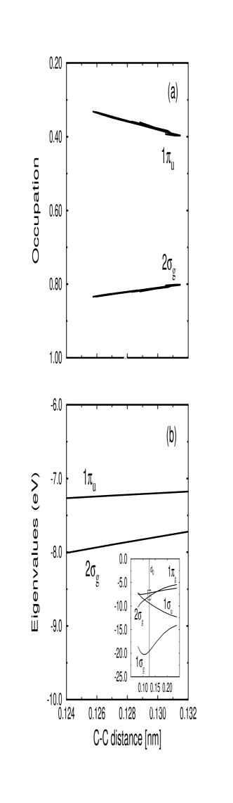
FIG. 4.: (a) Occupation numbers of the highest occupied molecular orbital $1\sigma_{\rm g}$ (HOMO, two-fold degenerate) and the lowest unoccupied molecular orbital (LUMO) $2\pi_{\rm u}$ as a function of the interatomic distance during the vibration of a carbon dimer, using $k_{B}T_{\text{el}}$=0.5 eV.
(b) Energy levels of a carbon dimer as a function of the interatomic distance. $d_{0}$ marks the quilibrium distance.

To complete our analysis, we also applied a more general method, for calculating $\partial f_{i}/\partial{\bf R}$. We will use again the Al slab as an example. At constant temperature and number of electrons, the occupation numbers $f_{i}$ depend on the one-electron energies $\epsilon_{i}$ and on the chemical potential $\mu$. Thus,

$$\frac{\partial f_{i}}{\partial{\bf R}}=\frac{\partial f_{i}}{\partial\epsilon_{i}}\left(\frac{\partial\epsilon_{i}}{\partial{\bf R}}-\frac{\partial\mu}{\partial{\bf R}}\right)\quad,$$ (12)

in which the chemical potential is obtained from the constraint that the $f_{i}$ sum up to the number of electrons. Because a given atomic displacement will result in an increase of some eigenvalues and a decrease of the other ones, the derivative of the chemical potential is smaller than those of the eigenvalues. It is nevertheless not negligible: in the case of the relaxation of Al (111), we find that the contribution of the derivative of the chemical potential is about 0.2 times that of the derivative of the eigenvalues.
Linear-response theory[12, 13, 14] enables us to calculate the quantities $\partial\epsilon_{i}/\partial{\bf R}$, which are the expectation values of $\partial\cal H/\partial{\bf R}$ for the eigenstates $\left|\psi_{i}\right\rangle$

$$\frac{\partial\epsilon_{i}}{\partial{\bf R}}=\left\langle\psi_{i}\left|\frac{\partial\cal H}{\partial{\bf R}}\right|\psi_{i}\right\rangle\quad.$$ (13)

Other methods would be more time-consuming and thus inadequate for the purpose of geometry optimization or MD, where the forces must be calculated for many different atomic configurations and sometimes for systems of 100 atoms and more. The dielectric matrix, for example, would require the calculation of many bands and the inversion of large matrices.
The explicit dependence of $\cal H$ on $\bf R$ is only in $V_{\text{ext}}$, but $V_{H}$ and $V_{\text{xc}}$ depend on the atomic positions through the electron density. For that reason, an evaluation of the forces not using the values of the $\epsilon_{i}$ of previous atomic positions requires a self-consistent calculation of the derivatives $\partial\epsilon_{i}/\partial{\bf R}$. Neglecting the dependence of $V_{H}$ and $V_{\text{xc}}$ on $\bf R$ to avoid the use of an iterative computation would result in unacceptable errors: in the example of the Al slab, we encountered cases where non self-consistent forces were too large by an order of magnitude.
The derivative of the electron density is given by

$$\frac{\partial n({\bf r})}{\partial{\bf R}}=2\sum_{i}\left\{\frac{\partial f_{i}}{\partial{\bf R}}\left|\psi_{i}({\bf r})\right|^{2}+2f_{i}\Re\left[\psi_{i}^{*}({\bf r})\frac{\partial\psi_{i}({\bf r})}{\partial{\bf R}}\right]\right\}\quad,$$ (14)

where the first term accounts for the redistribution of the electrons among the orbitals due to the variation of the $\epsilon_{i}$ and the second term comes from the modification of the wavefunctions. From the current approximation of $\partial\epsilon_{i}/\partial{\bf R}$, Eq. (12) is used to calculate the first term. The second term requires the resolution of

$$\left({\cal H}-\epsilon_{i}\right)\left|\frac{\partial\psi_{i}}{\partial{\bf R}}\right\rangle=-\left(\frac{\partial{\cal H}}{\partial{\bf R}}-\frac{\partial\epsilon_{i}}{\partial{\bf R}}\right)\left|\psi_{i}\right\rangle\quad.$$ (15)

Equation (15) is ill-conditioned, because the operator $\left({\cal H}-\epsilon_{i}\right)$ of the left-hand side has in general eigenvalues of either sign, some of them having small absolute values. Later in this paper (Eqs. 18 and 20), we are going to explain an iterative resolution method instrumental for positive-definite operators and which converges better if the eigenvalues of that operator are large. In order to make that method applicable to our problem, we separate the Hilbert space in two subspaces: the first one is spanned by the computed eigenstates, and the second one is its complementary subspace (spanned by unoccupied states). In practical calculations, only the $i_{\text{max}}$ lowest energy levels, including all occupied states and some unoccupied states, are computed and the occupation numbers are fractional only for the levels with energies $\pm k_{B}T_{\text{el}}$ around the Fermi level. Let $\cal P$ be the projector on the second subspace ($i>i_{\text{max}}$) and $\left|\partial\tilde{\psi}_{i}/\partial{\bf R}\right\rangle$ be ${\cal P}\left|\partial\psi_{i}/\partial{\bf R}\right\rangle$. Now, we can rewrite Eq. (14) as

$$\frac{\partial n({\bf r})}{\partial{\bf R}}=2\sum_{i=1}^{i_{\text{max}}}\left\{\frac{\partial f_{i}}{\partial{\bf R}}\left|\psi_{i}({\bf r})\right|^{2}+\right.$$

$$\left.2\sum_{j=i+1}^{i_{\text{max}}}\frac{f_{i}-f_{j}}{\epsilon_{i}-\epsilon_{j}}\Re\left[\left\langle\psi_{i}\left|\frac{\partial H}{\partial{\bf R}}\right|\psi_{j}\right\rangle\psi_{i}({\bf r})\psi_{j}({\bf r})^{*}\right]\right.$$

$$\left.+2f_{i}\Re\left[\psi_{i}({\bf r})\frac{\partial\tilde{\psi}_{i}({\bf r})^{*}}{\partial{\bf R}}\right]\right\}\quad.$$ (16)

Some of the differences $(\epsilon_{i}-\epsilon_{j})$ appearing in the denominator of the second term in Eq. (16) are small but, in that case, the difference between the occupation numbers in the numerator is small as well, so the whole fraction has a finite value.
The quantities $\left|\partial\tilde{\psi}_{i}/\partial{\bf R}\right\rangle$ are the solutions of

$$\left({\cal H}-\epsilon_{i}\right)\left|\frac{\partial\tilde{\psi}_{i}}{\partial{\bf R}}\right\rangle=-{\cal P}\frac{\partial\cal H}{\partial{\bf R}}\left|\psi_{i}\right\rangle\quad.$$ (17)

Since Eq. (17) is only for the subspace $i>i_{\text{max}}$, the operator $\left({\cal H}-\epsilon_{i}\right)$ is positive-definite. Moreover, an approximation $\cal D$ to $\left({\cal H}-\epsilon_{i}\right)$ can be obtained by neglecting its off-diagonal matrix elements. In the plane-wave basis set we use in the examples, this amounts to including the kinetic part of the hamiltonian and the average value of the effective potential. The algorithm introduced by Williams and Soler[15] can be generalized to solve Eq. (17) iteratively. An initial guess is given by

$$\left|\frac{\partial\tilde{\psi}_{i}^{(0)}}{\partial{\bf R}}\right\rangle=-{\cal D}^{-1}{\cal P}\frac{\partial\cal H}{\partial{\bf R}}\left|\psi_{i}\right\rangle$$ (18)

and the sequence of approximations is obtained using

$$\left|\frac{\partial\tilde{\psi}_{i}^{(n+1)}}{\partial{\bf R}}\right\rangle=\left|\frac{\partial\tilde{\psi}_{i}^{(n)}}{\partial{\bf R}}\right\rangle+{\cal P}{\cal D}^{-1}\left(1-e^{-\Delta{\cal D}}\right)$$ (19)

$$\left[(\epsilon_{i}-{\cal H})\left|\frac{\partial\tilde{\psi}_{i}^{(n)}}{\partial{\bf R}}\right\rangle-{\cal P}\frac{\partial\cal H}{\partial{\bf R}}\left|\psi_{i}\right\rangle\right]\quad.$$ (20)

In order to make the convergence as fast as possible, the largest value keeping the algorithm stable is chosen for the constant $\Delta$. The operators ${\cal D}^{-1}$ and $e^{-\Delta{\cal D}}$ are easily computed, because ${\cal D}$ is diagonal. The operator $\partial{\cal H}/\partial{\bf R}$ is different at each iteration, because the value of $\partial n({\bf r})/\partial{\bf R}$ on which it depends is updated each time, in order to make the charge redistribution converge to self-consistence. This is analogous to the method used for the total-energy minimization[16], where the convergence towards the self-consistent charge density and the diagonalization of the hamiltonian are performed simultaneously.
The method explained above was applied to the Al slab. The corrected force is plotted in Figure 2(c) and it indeed vanishes for the geometry that minimizes the zero-temperature total energy.

As expected from Eqs. (9) and (3), the dependence of the non-corrected force on $T_{\text{el}}$ is quadratic. Therefore it should be possible to extrapolate the force to the value at zero temperature from two points at finite temperature. Figure 1 (a) shows the result for the Al (111) slab, using 48 k-points in the irriducible part of the Brillouin zone. Using the formula

$${\bf F}^{\text{zero}}=\frac{dA(T_{1})/d{\bf R}-(T_{1}/T_{2})^{2}dA(T_{2})/d{\bf R}}{(T_{1}/T_{2})^{2}-1}$$ (21)

we obtain a value which matches quite well the nearly constant value, obtained for the entropy-corrected force and by the linear treatment. This extrapolation scheme even works for metals which are not free electron like, as it is shown in Figure 1 (b) for the case of platinum. In the case we used 69 k-points in the irriducible part of the Brillouin zone. As for a transition metal no broadening temperature above 0.1-0.2 eV should be used to retain the properties of the Fermi surface, in many cases there might be no need to correct the forces at all. But calculating the forces at two different temperatures and extrapolating to $T_{\rm el}=0$ may lead to some additional improvement.

Methfessel and Paxton[17] proposed an improved smearing scheme in which the orbitals are occupied according to a smooth approximation of the step function. The computed quantities (energy, forces,…) converge towards their zero-temperature values when the order of the approximation is increased. Unfortunately higher-order approximations become more and more wigglier and therefore require larger $\bf k$-point sets. In practical calculations therefore only the first order approximation is used. In Figure 1 the differences of the calculated energies for finite temperatures to the energy at zero temperature for the Al-111 (a) and the Pt-111 (b) slab is plotted as a function of the broadening parameter. For both systems the deviation of the energies obtained by using the first order Methefessel-Paxton scheme (full circles) ist comparable to that of the extrapolated energies (open squares) using the finite temperature approach (open diamonds).

Figure 5 shows that for both systems the error in the forces which are obtained when the Methefessel-Paxton scheme is used also is comparable to the error in the forces obtained by the quadratic extrapolation. But Figure 5 also shows, that the forces obtained by using the MP-scheme are wigglier, especially for the Al-111 slab, where only 48 k-Points have been used.

FIG. 5.: Non-corrected force acting on the first layer of a four layer (111) slab of aluminium (a) and platinum (b) as a function of the broadening energy $k_{B}T_{\text{el}}$ using a fermi-smearing (closed circles) and the Methfessel-Paxton-scheme of first order (closed squares). Parabolic fit (dotted line) and forces extrapolated to T=0 (open markers). Dashed line corresponds to the minimum of the parabola.

In conclusion, we have shown how the entropy arising from the broadening of the occupation numbers can be included in the calculation of the forces. For small distortions the dependences of the occupation numbers are linear to a good approximation. Thus, information from the history of the MD run can be used to determine $\partial f_{i}/\partial{\bf R}$. For the general case, e.g. when the needed information is not available from the history, we developed an iterative method based on the linear-response theory. The forces obtained in this way are the exact derivatives of the extrapolated zero-temperature energy. Neglecting the contribution of $V_{H}$ and $V_{\text{xc}}$ to $\partial\epsilon_{i}/\partial{\bf R}$, in other words stopping the calculation after the first iteration would result in unacceptably errors. If $\bf k$-point convergence is fulfilled, the corrected force is nearly independent of the broadening temperature in a wide temperature range. In that case, extrapolation to zero temperature from the results at two finite temperatures also gives good results.
Among the three methods presented in this paper, linear-response theory is the most general one: it is valid for any dependence of the one-electron energies on the atomic positions. On the other hand, this method is computationally very expensive, which limits it’s usefuleness in practical calculations. The extrapolation method requires the calculation of the forces for two different temperatures, which in general does not double the number of iterations, since the number of iterations needed is much smaller starting from a selfconsistent charge density at a different temperature. Therefore extrapolation from two different temperatures is more practical, especially if the number of degrees of freedom is large.
While the error in the forces is small compared to the usual accurancy in atomic relaxations, and therefore might be neglected if the broadening temperature is choosen carefully, the correction is especially important to stay consistent in a molecular dynamics simulation, where the quantity to be conserved should be the ground state energy of the electronic system and not the unphysical free energy of the electronic system, which is excited due to the broadening.

Using the scheme proposed by Methfessel and Paxton in it’s first order approximation leads to energies, which are comparable to the energies obtained by extrapolating the finite temperature energies to $T_{\rm el}=0$. The calculated forces are the derivatives of these energies and need no further correction.

REFERENCES

- [1] D.J. Chadi and M.L. Cohen, Phys. Rev. B 8, 5747 (1973).
- [2] H.J. Monkhorst and J.D. Pack, Phys. Rev. B 12, 5188 (1976).
- [3] C.-L. Fu and K. .M. Ho, Phys. Rev. B 28, 5480 (1983).
- [4] N.D. Mermin, Phys. Rev. 137, A 1441 (1969).
- [5] M. Weinert and J.W. Davenport, Phys. Rev. B 45, 13709 (1992).
- [6] N. W. Ashcroft and N. D. Mermin, Solid State Physics (Saunders College, Philadelphia, 1976), pg. 47.
- [7] M. G. Gillan, J. Phys. Condens. Matter 1, 689 (1989).
- [8] J. Neugebauer and M. Scheffler, Phys. Rev. B 46, 16067 (1992).
- [9] D. R. Hamann, Phys. Rev. B 40, 2980 (1989).
- [10] X. Gonze, R. Stumpf and M. Scheffler, Phys. Rev. B 44, 8503 (1991).
- [11] D. J. Chadi and M. L. Cohen, Phys. Rev. B 8, 5747 (1973).
- [12] S. Baroni, P. Giannozzi, and A. Testa, Phys. Rev. Lett. 58, 1861 (1987).
- [13] S. Baroni, P. Giannozzi, and A. Testa, Phys. Rev. Lett. 59, 2662 (1987).
- [14] X. Gonze and J.-P. Vigneron, Phys. Rev. B 39, 13120 (1989).
- [15] A. Williams and J. Soler, Bull. Am. Phys. Soc. 32, 562 (1987).
- [16] M. C. Payne, M. P. Teter, D. C. Allan, T. A. Arias, and J. D. Johannopoulos, Rev. Mod. Phys. 64, 1045 (1992).
- [17] M. Methfessel and A. T. Paxton, Phys. Rev. B 40, 3616 (1989).