Simulated Dynamics of Underpotential Deposition of Cu with Sulfate on Au(111)

Abstract

Numerical studies of lattice-gas models are well suited to describe multi-adsorbate systems. One example is the underpotential deposition of Cu on Au(111) in the presence of sulfuric acid. Preliminary results from dynamic Monte Carlo simulations of the evolution of the adsorbed layer during potential-step experiments across phase transitions are presented for this particular system. The simulated current profiles reproduce a strong asymmetry seen in recent experiments. Examination of the microscopic structures that occur during the simulated evolution processes raises questions that need to be investigated by further experimental and theoretical study.

Keywords: Underpotential deposition. Multi-adsorbate systems. Lattice-gas model. Butler-Volmer approximation. Dynamic Monte Carlo simulation.

1 Introduction

Underpotential deposition (UPD) provides a window of electrode potentials in which a monolayer or less of one metal can be deposited onto the surface of another metal. Recently, experiments that probe the dynamical properties of the adsorption process [1] have also added to our knowledge of UPD monolayers. Here we present preliminary results for dynamical simulations of a microscopic model which reproduce the results of potential-step experiments and make microscopic predictions that may be testable by modern in-situ experimental techniques, such as scanning-probe microscopy and synchrotron X-ray scattering.

The UPD of copper onto gold single-crystal electrodes in the presence of sulfate is a particularly well studied model system. See, for example, the review of the experimental literature in Ref. [2]. For this system cyclic voltammograms, like the one shown in Fig. 1, show two current peaks corresponding to two different transitions in the surface structure [3]. Scanning-tunneling microscopy (STM) [4, 5] and low-energy electron diffraction (LEED) [2] studies indicate that these transitions occur between a full monolayer (ML) of Cu at more negative potentials, an ordered $(\sqrt{3}\times\sqrt{3})$ mixed copper and sulfate phase at intermediate potentials, and a disordered low-coverage phase at more positive potentials. In situ X-ray scattering confirms that the ordered phase consists of a 2/3 ML of copper in a honeycomb pattern, with a 1/3 ML of sulfate occupying the remaining adsorption sites [6], as originally proposed by Huckaby and Blum [7].

An effective theoretical approach for understanding a multi-species layer chemisorbed on a surface is to study a statistical-mechanical lattice-gas model numerically. Such models describe the adsorbate layer by a Hamiltonian which gives the energies of different adsorbate configurations. Early studies [7, 8, 9] together with later applications to problems such as the adsorption of urea on Pt(100) [10, 11] and the UPD of Cu with sulfate on Au(111) [2, 7], in or near equilibrium, are discussed in recent review articles [12, 13, 14]. In particular, that work provided estimates for effective lateral interaction energies, based on comparison of the theoretical predictions with experimentally observed equilibrium adsorption isotherms and voltammetric currents for small potential sweep rates.

Dynamical properties of the copper UPD system have recently been investigated by Hölzle, Retter, and Kolb (HRK) [1]. They measured current transients in potential-step experiments performed at both transitions and with both positive-going and negative-going steps. In this article we report current transients and time-dependent microscopic adlayer structures observed in dynamic Monte Carlo simulations of a model UPD system under conditions intended to reproduce those experiments. In a previous study [15], our model agreed qualitatively with the experiments only for steps across one transition, the mixed-disordered phase transition marked ${\rm A}$ and ${\rm A}^{\prime}$ in Fig. 1. Reproducing the behavior seen for potential steps across both transitions represents a significant refinement of the lattice gas model. Our microscopic predictions indicate the desirability of time-resolved, structurally sensitive, in situ experimental studies of this system.

2 Lattice-gas Model

Our theoretical lattice-gas model treats copper and sulfate as interacting particles that compete for the same adsorption sites. For the Au(111) surface this is a triangular lattice of threefold hollow sites [6]. The model is defined by the effective lattice-gas Hamiltonian,

$${\mathcal{H}} = -\sum_{n}\left[\Phi_{\rm CC}^{(n)}\sum_{\langle ij\rangle}^{(n)}c_{i}^{\rm C}c_{j}^{\rm C}+\Phi_{\rm CS}^{(n)}\sum_{\langle ij\rangle}^{(n)}\left(c_{i}^{\rm C}c_{j}^{\rm S}+c_{i}^{\rm S}c_{j}^{\rm C}\right)+\Phi_{\rm SS}^{(n)}\sum_{\langle ij\rangle}^{(n)}c_{i}^{\rm S}c_{j}^{\rm S}\right]$$

$$-\Phi_{\rm SS}^{(t)}\sum_{\triangle}c_{i}^{\rm S}c_{j}^{\rm S}c_{k}^{\rm S}-\sum_{i}\bar{\mu}_{\rm C}c_{i}^{\rm C}-\sum_{i}\bar{\mu}_{\rm S}c_{i}^{\rm S}\;.$$

Here $c_{i}^{\rm X}$ equals unity when lattice site $i$ is occupied by species ${\rm X}$, with ${\rm X}={\rm C}$ for copper and ${\rm X}={\rm S}$ for sulfate; otherwise $c_{i}^{\rm X}$ equals zero. This third state represents sites solvated by water. The effective interaction for $n$-th neighbor adsorbates ${\rm X}$ and ${\rm Y}$ is $\Phi_{\rm XY}^{(n)}$, and $\sum_{\langle ij\rangle}^{(n)}$ represents the sum over all $n$-th order neighbor pairs. We also include a three-body interaction, $\Phi_{\rm SS}^{(t)}$, for equilateral triangles of sulfate adsorbed on second-neighbor sites. The sum over all possible triangles is denoted by $\sum_{\triangle}$. Finally, $\bar{\mu}_{\rm X}$ is the electrochemical potential for ${\rm X}$, and $\sum_{i}$ is the sum over all lattice sites. Attractive interactions are represented by positive quantities, and positive electrochemical potentials indicate a preference for adsorption in the absence of lateral interactions.

The quantities $\Phi_{\rm XY}^{(n)}$ in the lattice-gas model are effective parameters representing the joint effect of competing, unspecified interaction potentials. Ground-state calculations can be used to determine multi-dimensional regions of parameter space that give phase diagrams that agree with the phases observed experimentally. Fitting the model to a particular system involves an iterative process of selecting experiments and adjusting the parameters to achieve improved agreement. The expectation is that the model will more accurately represent the real chemical system as it correctly reproduces and predicts an ever wider range of experimental observations. Detailed discussion of the methods used to estimate the effective interaction constants are given in Refs. [2, 11, 12].

The effective interactions used in the present study are illustrated in Fig. 2. There, and elsewhere in this paper, unoccupied adsorption sites are represented by an open circle ($\circ$), sites occupied by copper are represented by a filled circle ($\bullet$), and those occupied by sulfate are represented by a triangle ($\triangle$). These interactions have been adapted from those of Ref. [2]. Changes in the sulfate-sulfate interactions removed from the ground-state diagram three experimentally unobserved low-temperature phases which were overlooked in Ref. [2]. Strengthening the attractive next-nearest neighbor copper-copper interaction, $\Phi_{\rm CC}^{(2)}$, was required to make the phase transition between the copper monolayer and the mixed phase (peaks ${\rm B}$ and ${\rm B}^{\prime}$ in Fig. 1) first order and produce current transients for this transition in qualitative agreement with experiments (described in Sec. 4).

The ground-state diagram for the interactions of Fig. 2 is presented in Fig. 3, and the geometries of the main observed phases are illustrated in Fig. 4. Here the phases are labeled by the length of their basis vectors and subscripted (superscripted) by the fraction of sites filled by copper (sulfate).

The electrochemical potential of species ${\rm X}$ is controlled through its bulk solution activity and the electrode potential, $E$. In the weak-solution limit, the activity equals the solute molar concentration $[{\rm X}]$. Then the electrochemical potential, $\bar{\mu}_{\rm X}$, is

$$\bar{\mu}_{\rm X}=\mu_{\rm X}^{0}+RT\ln{\frac{[{\rm X}]}{[{\rm X}]^{0}}}-z_{\rm X}FE,$$ (2)

where $z_{\rm X}$ is the effective electrovalence of ${\rm X}$, $F$ is Faraday’s constant, $R$ is the molar gas constant, $T$ is temperature, and the reference state is ${\mu}_{\rm X}^{0}$, $[{\rm X}]^{0}$, and $E^{0}=0$. For fixed $[{\rm S}]$ and $[{\rm C}]$, Eq. (2) for $\bar{\mu}_{\rm S}$ and $\bar{\mu}_{\rm C}$ form the parametric representation of a line in the ground-state diagram. The electrode potential $E$ is the parameter that determines the location along this isotherm, whose slope is $z_{\rm S}/z_{\rm C}$. We have chosen an isotherm such that the potential difference between the two transitions is the same as observed by HRK. Its location is given by the dotted line in Fig. 3 for $0\leq E\leq 350{\rm mV}$ vs Ag/AgCl.

3 Dynamic Monte Carlo Method

The equilibrium properties of a lattice-gas Hamiltonian can often only be practically evaluated using Monte Carlo methods, by which thermodynamic average values are calculated from a representative sampling of the equilibrium states. This sampling is generated using the principle of detailed balance: in equilibrium the rate of going from configuration $A$ to configuration $B$ is equal to the rate of going from $B$ to $A$. Many Monte Carlo techniques generate new configurations through a series of Monte Carlo steps, each step consisting of a proposed small change in the configuration which is accepted or rejected according to an acceptance probability that must satisfy detailed balance.

A lattice-gas Hamiltonian merely provides the free energies corresponding to different geometric configurations of the adsorbate layer. In contrast to a quantum-mechanical Hamiltonian, it does not possess an intrinsic dynamic. However, when Monte Carlo steps are associated with a discrete unit of time, the simulation can be viewed as a “movie” of a dynamic process.

Many different Monte Carlo algorithms can be designed to describe the equilibrium properties of a particular system. In general such an algorithm does not realistically describe the dynamics of a particular chemical system. But if care is taken to include only dynamically realistic moves in the algorithm, it is possible to construct a Monte Carlo dynamic which simulates that of the real system under consideration. This should be the case when the real dynamics is well approximated by a stochastic process on the timescales of interest. The example relevant to our present discussion is the thermally activated motion of particles adsorbing onto, desorbing from, and diffusing between adsorption sites on the electrode surface. This view of Monte Carlo simulation can be combined with the lattice-gas Hamiltonian to construct a stochastic dynamic describing the individual motions of specific adsorbate particles. An introduction to Monte Carlo methods for equilibrium and nonequilibrium problems in surface electrochemistry is given in Ref. [16].

Here we construct a microscopic dynamic which includes adsorption, desorption, and one-step lateral diffusion of both adsorbate species. The rate of each process is determined using a simple Arrhenius picture, with all processes having the same pre-exponential factor $\nu_{0}$. The free energy associated with an adsorbed particle of species ${\rm X}$ occupying site $i$ for a specific configuration of neighbors is given by

$${\mathcal{H}}_{i}({\rm X};\Gamma)=-\sum_{n}\left[\Phi_{\rm XC}^{(n)}\sum_{j(i)}^{(n)}c_{j}^{\rm C}+\Phi_{\rm XS}^{(n)}\sum_{j(i)}^{(n)}c_{j}^{\rm S}\right]-\delta_{\rm X,S}\Phi_{\rm SS}^{(t)}\sum_{\triangle(i)}c_{j}^{\rm S}c_{k}^{\rm S}-\bar{\mu}_{\rm X}\;,$$ (3)

where $\sum_{j(i)}^{(n)}$ represents the sum over all adsorption sites $j$ that are $n$-th neighbors of site $i$, and $\sum_{\triangle(i)}$ is the sum over all second-neighbor equilateral triangles involving site $i$. The factor $\delta_{\rm X,S}$ is unity when ${\rm X}={\rm S}$ and zero otherwise. The index $\Gamma$ runs over all possible arrangements of neighboring adsorbate particles within the maximum interaction range from site $i$. When the site is empty and the ion is in solution, the free energy is defined to be zero. Using ${\rm X}=0$ to denote an unoccupied site, ${\mathcal{H}}_{i}(0;\Gamma)=0$, regardless of the arrangement of the neighbors.

The energy barriers are assumed to vary according to the Butler-Volmer approximation [17]. Specifically, consider the adsorption-desorption processes for a particular site. A schematic free-energy surface is shown in Fig. 5(a), assuming three different arrangements of neighbors, $\Gamma$. If ${\mathcal{H}}_{i}({\rm X};\Gamma)=0$, there is no preference toward adsorption, but there is still a transition-state free energy, $\Delta^{*}_{0}({\rm X})$. The transition-state free energy for this case is used as the reference value for the adsorption transition energy for all configurations of the neighbors. If a site has no neighbors within the maximum interaction range, the free energy of the adsorbed particle is controlled by the electrochemical potential and equals $-\bar{\mu}_{\rm X}$. In the Butler-Volmer approximation, the transition energy for adsorption to that site is then lowered from $\Delta^{*}_{0}({\rm X})$ by an amount $\alpha\bar{\mu}_{\rm X}$. Here $\alpha$ is the symmetry factor, which is often close to $1/2$. For the present model, lateral interactions with neighboring ions are also important. If the net lateral interactions are attractive, the free energy corresponding to the adsorbed state lies below $-\bar{\mu}_{\rm X}$, as illustrated by the lowest adsorbed free-energy level in Fig. 5(a). If the net lateral interactions are repulsive, the free energy is raised above $-\bar{\mu}_{\rm X}$. Our generalization of the Butler-Volmer approximation uses the total free energy gained to calculate the free-energy barrier for adsorption, specifically

$$\Delta^{*}_{i}({\rm X};\Gamma)=\Delta^{*}_{0}({\rm X})+\alpha{\mathcal{H}}_{i}({\rm X};\Gamma)\;.$$ (4)

Using the same transition-state energy $\Delta^{*}_{i}({\rm X};\Gamma)$ for the adsorption and desorption process is essential for Monte Carlo simulations in order to satisfy detailed balance and thus ensure eventual approach to thermodynamic equilibrium. In the model developed here, an ion approaching the surface from the solution sees different free-energy barriers for sites with different arrangements of neighbors. Adsorption on a site is faster when its neighbors help lower the free energy of the adsorbed state; conversely, desorption from such a site is relatively slow. For multi-component adsorption, the adsorption of one species may be much faster than that of the other at a particular site.

For lateral diffusion from one adsorption site to another, a slightly modified approach is needed. The situation for two neighboring sites, both with favorable adsorption free energies, is shown in Fig. 5(b). The difficultly is that detailed balance requires a single transition-state free energy, $\tilde{\Delta}^{*}_{ij}({\rm X};\Gamma)$, between the two sites. An obvious solution would be to adjust the energy barrier by the average of the free energies for the two sites, $({\mathcal{H}}_{i}({\rm X};\Gamma)+{\mathcal{H}}_{j}({\rm X};\Gamma))/2$ [18]. Unfortunately this could lead to ${\mathcal{H}}_{i}({\rm X};\Gamma)<\tilde{\Delta}^{*}_{ij}({\rm X};\Gamma)<{\mathcal{H}}_{j}({\rm X};\Gamma)$, which violates the usual definition of a transition-state free energy. To avoid this, we use the least favorable adsorption free energy for calculating the transition-state free energy for diffusion between nearest-neighbor sites $i$ and $j$:

$$\tilde{\Delta}^{*}_{ij}({\rm X};\Gamma)=\tilde{\Delta}^{*}_{0}({\rm X})+\frac{1}{2}{\rm Max}({\mathcal{H}}_{i}({\rm X};\Gamma),{\mathcal{H}}_{j}({\rm X};\Gamma))\;.$$ (5)

Violations of the transition-state picture are minimized because they involve very unfavorable sites, which are only rarely occupied. The barrier for diffusion to each neighbor is calculated individually; diffusion into a less favorable site will be relatively slow. Diffusion to an occupied site is forbidden and has a rate identically zero. For our simulations, we choose the transition-state free energies as $\Delta^{*}_{0}({\rm C})=50\,{\rm kJ/mol}$ for copper adsorption, $\Delta^{*}_{0}({\rm S})=55\,{\rm kJ/mol}$ for sulfate adsorption, and $\tilde{\Delta}^{*}_{0}({\rm C})=\tilde{\Delta}^{*}_{0}({\rm S})=35\,{\rm kJ/mol}$ for diffusion of both species. These choices make adsorption faster for copper than sulfate and allow relatively long diffusion paths across the surface since diffusion is faster than adsorption. We take the symmetry factor $\alpha=1/2$.

The rates described above can be used to implement a rejection-free Monte Carlo algorithm [16, 19]. A list of all the single-ion processes is maintained. Each process is weighted by its rate, so that making a random choice from the list is biased towards the faster processes. Each simulation step consists of choosing a process from the weighted list, making the appropriate change to the system, and recalculating the weights for the list. At each step the simulation clock is updated by a random number that represents the elapsed time since the last move. For a given configuration the overall rate for the system to change by some microscopic process is the sum of all the individual microscopic process rates. Since the decay of a particular state has a constant rate, the elapsed time for the actual change has an exponential distribution. Results for a simplified model were presented in Ref. [20].

Our simulations were conducted on $30\times 30$ parallelograms of a triangular lattice with periodic boundary conditions. A particular potential-step simulation involves equilibration for a fixed time at one potential. Then, at time $t=0$, the applied potential is changed to its final value, and measurements of the partial coverage due to each species are made at fixed simulation times after the quench. Results reported here are averaged over at least 1000 individual simulations. Currents are calculated by numerical differentiation of the coverage with respect to time, with electrovalences of $z_{\rm S}=-0.9$ and $z_{\rm C}=+1.54$ [2]. The natural simulation time unit is Monte Carlo steps per site (MCSS), but choosing $\nu_{0}=2\times 10^{9}\;{\rm MCSS}\,{\rm s}^{-1}$ makes the scale of simulated currents agree roughly with experiments. The rejection-free algorithm is essential, since achieving a time scale of $10^{9}\;{\rm MCSS}$ would be prohibitive for a traditional Monte Carlo algorithm. Even with the rejection-free algorithm, some of the individual experiments took $15$ minutes to simulate on a DEC-Alpha workstation.

4 Results

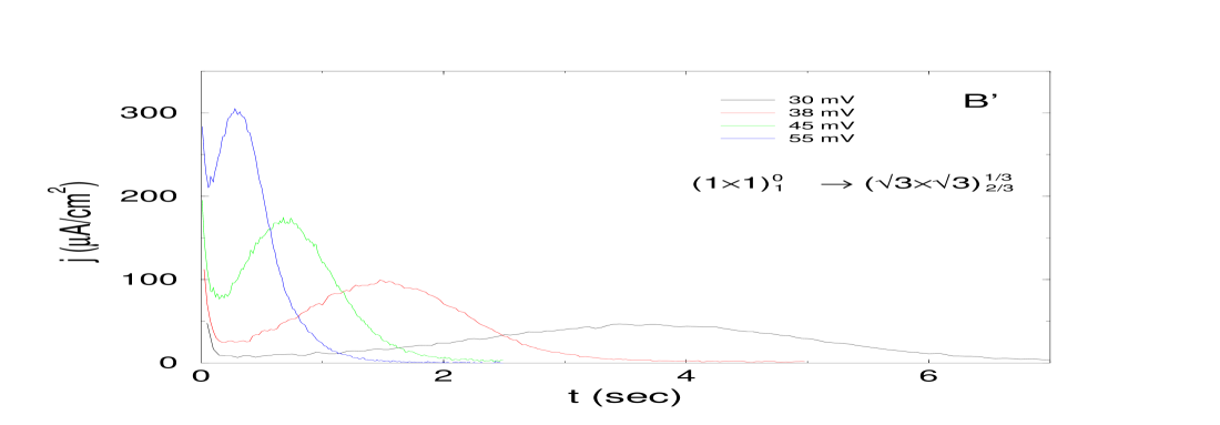
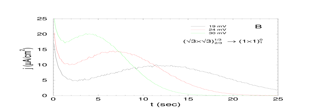
Figure 6: Simulated current transients after potential steps across the transition between the $(1\times 1)^{0}_{1}$ and $(\sqrt{3}\times\sqrt{3})^{1/3}_{2/3}$ phases. Positive (top) and negative (bottom) potential steps, ${\rm B}^{\prime}$ and ${\rm B}$, respectively, of HRK [1] are shown. The shape of the current profile corresponds to the decay of a metastable adsorbed layer. The trend for the broad maxima to shift to earlier times and larger amplitudes as the potential step is increased agrees with the experiments. The legend indicates the size of the potential step past the transition, $|E_{\rm final}-E_{\rm transition}|$. This figure should be compared with Fig. 3 of Ref. [1].

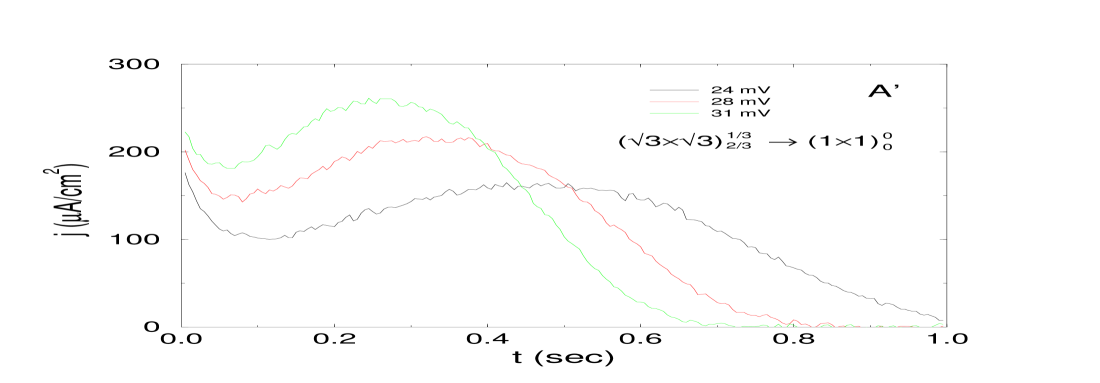
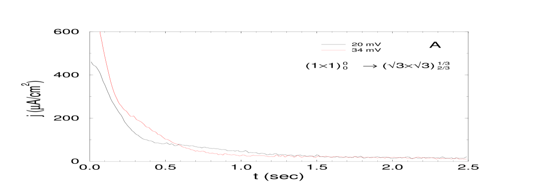
Figure 7: Simulated current transients after potential steps across the disorder-mixed transition for positive (top) and negative (bottom) potential steps, ${\rm A}^{\prime}$ and ${\rm A}$, respectively, of HRK [1]. The strong asymmetry in current profiles for the two step directions is seen experimentally. The broad maximum is characteristic of the decay of a metastable adsorbed layer, the monotonically decreasing initial current reflects the unstable nature of the low-coverage surface after a negative potential step. The legend indicates the size of the potential step past the transition, $|E_{\rm final}-E_{\rm transition}|$. This figure should be compared with Fig. 3 of Ref. [1].

The agreement between our simulations and the experiments of HRK [1] is encouraging (see Figs. 6 and 7). The current profiles, consisting of a rapid initial decay followed by a broad maximum at a later time, are characteristic of the decay of an adsorbed layer that is metastable after a potential step across a first-order phase transition. The initial current transient corresponds to the rapid relaxation to a long-lived metastable state which has only a small concentration difference from the adsorbate layer as it existed before the potential was changed. The second, broader current maximum occurs as domains of the equilibrium phase nucleate and grow. This behavior is seen for three of the four potential steps.

The simulated current transients for potential steps around the transition between the $(1\times 1)^{0}_{1}$ and $(\sqrt{3}\times\sqrt{3})^{1/3}_{2/3}$ phases, labelled ${\rm B}$ and ${\rm B}^{\prime}$ in Figs. 1 and 3, are shown in Fig. 6. Both reflect one-step nucleation and growth mechanisms. Following the trend seen in the experimental data, the broad maximum becomes stronger and the maximum shifts to earlier times as the size of the step is increased. However, the time corresponding to the second maximum appears to depend more strongly on the step size than observed in the experiments.

The current transients observed for the transition between the $(\sqrt{3}\times\sqrt{3})^{1/3}_{2/3}$ and the disordered low-coverage phases, labelled ${\rm A}$ and ${\rm A}^{\prime}$ in Figs. 1 and 3, are very different for positive and negative potential steps, as seen in Fig. 7. This was also observed by HRK. When the potential is increased from the ordered-phase region into the disordered-phase region, a step corresponding to ${\rm A}^{\prime}$, the current profile has the broad maximum, similar to those shown in Fig. 6. Again, the qualitative trend seen for the strength and location of the second current maximum as the size of the step is changed agrees with the experiments. In contrast to our previous simulations, which were performed for a system with different interactions [15], this current is caused by the decay of the metastable $(\sqrt{3}\times\sqrt{3})_{2/3}^{1/3}$ phase to the $(\sqrt{3}\times\sqrt{3})_{1/3}^{1/3}$ phase, which is also metastable. The decay of this second metastable phase to the final low-coverage phase takes place at much later times, but causes a current transient with a much smaller amplitude because the copper and sulfate currents have opposite sign. Both metastable phases decay by a nucleation and growth mechanism.

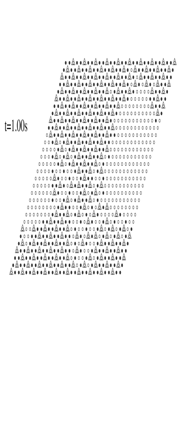
Figure 8: A series of snapshots after a negative-going potential step to 20mV below the transition between the low coverage and mixed layers. After the step, a fraction of the sulfate desorbs, but the remaining sulfate combines with the newly adsorbed copper to form a loose domain. With time this domain fills in and grows. The current transient is monotonically decreasing, as shown in Fig. 7, ${\rm A}$. Movies of the dynamics after the quench are available in MPEG format at http://www.scri.fsu.edu/~rikvold

The current profiles observed for potential steps in the negative direction, corresponding to peak ${\rm A}$, are qualitatively different than the other profiles. They are monotonically decreasing and do not correspond to a simple functional form. A sequence of configurations after a potential step to $20\,{\rm mV}$ below the transition is shown in Fig. 8. Because the applied potentials of HRK have been used, the equilibration occurs in a disordered phase with a relatively high sulfate coverage of approximately $0.25$ ML. After the potential step, copper adsorbs quickly onto the surface. The sulfate already present collapses with this copper to form a domain of the $(\sqrt{3}\times\sqrt{3})_{1/3}^{1/3}$ phase. Later this fills in with copper, forming the equilibrium $(\sqrt{3}\times\sqrt{3})_{2/3}^{1/3}$ phase. The adsorption of sulfate is an even slower process, which controls the shrinking of the domains of unoccupied sites. This process is different from our previous simulations [15], where no domain formation was observed. Instead, copper adsorbed into a loose network with open sites favorable for sulfate adsorption.

The fact that different dynamical paths can give current profiles qualitatively similar to those observed experimentally indicates that more study of the copper UPD system is desirable. Particularly useful would be time-resolved experiments that can probe the microscopic structure of the adsorbed layer. For the simulations, the factors controlling the different dynamical behaviors are not clearly understood and a more thorough investigation is needed.

5 Conclusions

Preliminary dynamic Monte Carlo simulation results are reported for potential step experiments for UPD of copper with sulfate on Au(111). The simulated current transients display the same general characteristics as those observed experimentally by Hölzle, Retter, and Kolb [1]. The current profiles for potential steps across the transition separating the copper monolayer and the ordered mixed phase (the transition marked ${\rm B}$ and ${\rm B}^{\prime}$ in Fig. 3) show a sharp initial transient followed by a broad second maximum that shifts to earlier times and larger amplitudes as the size of the step is increased. This contrasts with the asymmetry of the current profiles for potential steps across the transition separating the ordered mixed phase from the disordered low-coverage phase (the transition marked ${\rm A}$ and ${\rm A}^{\prime}$ in Fig. 3), where the second maximum is only seen for positive-going steps. Negative potential steps produce a monotonically decreasing current. We find that reproducing the profiles of HRK is not sufficient for determining the underlying dynamical process. For two slightly different models we have observed different processes occurring after the step. For both the negative-going and positive-going steps at this transition (${\rm A}$ and ${\rm A}^{\prime}$), an intermediate ordered phase with only $1/3$ monolayer of copper is observed in the model presented here that was not observed for an earlier model. In addition, domain formation is seen for negative steps. This was not observed in our simulations of the earlier model. Experiments which can dynamically monitor the microscopic structure of the adsorbate layer during the relaxation after the potential step would be useful in guiding further model development.

Figure 1: Cyclic voltammogram for Cu UPD onto Au(111) surface, after Ref. [2]. The two peaks correspond to two first-order phase transitions in the adsorbed layer. The arrows indicate the direction of the potential scan.

Figure 2: Diagrams illustrating the relative adsorbate positions corresponding to the $n$-th neighbor interactions, $\Phi_{\rm XY}^{(n)}$, in the lattice-gas model. Here Cu is represented by a filled circle ($\bullet$), sulfate is represented by a triangle ($\triangle$), and unoccupied sites are open circles ($\circ$). The interaction energy in ${\rm kJ/mol}$ is given below each diagram. Positive values indicate attractive interactions. First-neighbor sulfates are subject to an infinitely strong repulsion, i.e. configurations with first-neighbor sulfates are forbidden. The lower right-most diagram illustrates the three-body sulfate interaction. Note that some of the interactions are different from those used in Ref. [2].

Figure 3: The ground-state phase diagram (solid lines) for the lattice-gas model with interactions as given in Fig. 2. The axes represent the electrochemical potentials of the sulfate and copper, $\bar{\mu}_{\rm S}$ and $\bar{\mu}_{\rm C}$, respectively. The isotherm (dotted line) used for the simulated potential-step experiments was chosen to match the transition potentials observed in the experiments of HRK [1]. The geometries of the different phases are illustrated in Fig. 4.

Figure 4: Important phases observed for the present lattice-gas model of copper and sulfate adsorption on Au(111). Cu is represented as a filled circle ($\bullet$), sulfate as a triangle ($\triangle$), and empty sites as an unfilled circle ($\circ$). The label indicates the length of the unit vectors. The subscript and superscript represent the fraction of sites occupied by copper and sulfate, respectively. Two sulfate-free copper phases, $(\sqrt{3}\times\sqrt{3})_{1/3}^{0}$ and $(\sqrt{3}\times\sqrt{3})_{2/3}^{0}$, occur for this model at large negative $\bar{\mu}_{\rm S}$, but are not shown. Their geometries are easily deduced from the phases that are shown.

Figure 5: Butler-Volmer type free-energy barrier scheme. See text for details.

References

- [1] M. H. Hölzle, U. Retter, and D. M. Kolb, J. Electroanal. Chem., 371 (1994) 101.
- [2] J. Zhang, Y.-E. Sung, P. A. Rikvold, and A. Wieckowski, J. Chem. Phys., 104 (1996) 5699.
- [3] J. W. Schultze and D. Dickertmann, Surf. Sci., 54 (1976) 489.
- [4] T. Hachiya, H. Honbo, and K. Itaya, J. Electroanal. Chem., 315 (1991) 275.
- [5] O. M. Magnussen et al., J. Vac. Sci. Tech. B, 9 (1991) 969.
- [6] M. F. Toney et al., Phys. Rev. Lett., 75 (1995) 4472.
- [7] D. A. Huckaby and L. Blum, J. Electroanal. Chem., 315 (1991) 255.
- [8] P. A. Rikvold, J. B. Collins, G. D. Hansen, and J. D. Gunton, Surf. Sci., 203 (1988) 500.
- [9] L. Blum, Adv. Chem. Phys., 78 (1990) 171.
- [10] M. Gamboa-Aldeco et al., Surf. Sci., 297 (1993) L135.
- [11] P. A. Rikvold et al., Surf. Sci., 335 (1995) 389.
- [12] P. A. Rikvold, Electrochim. Acta, 36 (1991) 1689.
- [13] P. A. Rikvold, J. Zhang, Y. E. Sung, and A. Wieckowski, Electrochim. Acta, 41 (1996) 2175.
- [14] L. Blum, D. A. Huckaby, and M. Legault, Electrochim. Acta, 41 (1996) 2207.
- [15] P. A. Rikvold, G. Brown, M. A. Novotny, and A. Wieckowski, Colloids and Surfaces A, 134 (1998) 3.
- [16] G. Brown, P. A. Rikvold, S. J. Mitchell and M. A. Novotny, in Interfacial Electrochemistry, edited by A. Wieckowski, Marcel Dekker (New York, in press).
- [17] A. J. Bard and L. R. Faulkner, Electrochemical Methods: Fundamentals and Applications, Wiley (New York, 1980).
- [18] I. Vattulainen, J. Merikoski, T. Ala-Nissilä, and S. C. Ying, Surf. Sci., 366 (1996) L697.
- [19] M. A. Novotny, Computers in Physics, 9 (1995) 46.
- [20] P. A. Rikvold, A. Wieckowski, and R. A. Ramos, Mater. Res. Soc. Symp. Proc. Ser., 451 (1997) 69.