Static and Dynamic Properties of
Inhomogeneous Elastic Media on Disordered Substrate

Abstract

The pinning of an inhomogeneous elastic medium by a disordered substrate is studied analytically and numerically. The static and dynamic properties of a $D$-dimensional system are shown to be equivalent to those of the well known problem of a $D$-dimensional random manifold embedded in $(D+D)$-dimensions. The analogy is found to be very robust, applicable to a wide range of elastic media, including those which are amorphous or nearly-periodic, with local or nonlocal elasticity. Also demonstrated explicitly is the equivalence between the dynamic depinning transition obtained at a constant driving force, and the self-organized, near-critical behavior obtained by a (small) constant velocity drive.

]

I Introduction

The pinning of elastic continuum in random potential has been a subject of numerous studies in the past decade [2]. It is related to various phenomena of technological importance, while being also of fundamental interest to the statistical mechanics of disordered systems. Considerable efforts have been devoted to understanding how quenched impurities influence the transport of charge-density wave (CDW) [3, 4, 5], pinning of flux lines in type-II superconductors [6], roughness of crystalline surfaces [7, 8], propagation of invasion fronts [9], etc. Many aspects of these systems can be described either by the model of randomly-pinned CDW or by the model of randomly-pinned directed manifold (“random manifold” for brevity). The static properties of the low-temperature glass phases of these systems have been studied by a variety of analytical methods, including renormalization-group (RG) analysis [10, 11], replica variational method [12, 13], and functional RG [14, 15, 13]. Combined with the exact ground state structures obtained numerically via efficient (polynomial) algorithms [16, 17, 18, 19], these systems are perhaps the best characterized glassy system to date. Much progress have also been made in understanding the nonequilibrium driven dynamics of these systems [2]. In the extreme nonequilibrium limit where thermal fluctuations can be neglected, it is known that the driving force exceeding a critical value is necessary to depin the system. A continuous dynamic phase transition occurs at the depinning threshold, where the dynamics exhibits complex stick-slip motion with “avalanches” of all sizes. Such complex dynamics results from the intricate balance of elasticity and random pinning forces near the onset of motion. They have been characterized in great details by a combination of analytic [5, 20, 21, 22], numeric [23, 24, 25, 26, 27, 28, 29, 30], and experimental [31, 32, 33, 34, 35] methods.

Another class of pinning phenomena which have attracted much attention is the tribology of sliding elastic bodies interacting via a contact surface. This is exemplified by the Burridge-Knopoff model [36, 37, 38, 39] describing the dynamics along an individual earthquake fault. Other examples include boundary layer lubrication [40], and stick-slip motion [41, 42] of elastic continuum over sticky substrates. Complex spatio-temporal dynamics are found to occur in these systems also, when they are driven slowly. Previous studies [43] of this class of systems have focused on the role of chaos generated by nonlinear dynamics, e.g., a velocity-weakening friction. Complexity in these systems are not as well understood theoretically.

Another approach to studying the spatio-temporal complexity generated in tribology-like problems is by “sandpile”-like automaton models, as pioneered by Bak and collaborators [44, 45]. The connection between sandpile-like models and dynamic critical phenomena has been proposed early on by Tang and Bak [46]. (In fact, the sandpile model [47] itself was motivated from the study of the randomly-pinned CDW [48]. Equivalence between many aspects of the sandpile model and those of the CDW at the depinning threshold has since been verified numerically by Narayan and Middleton [49].) Analogy between the geometrical structures of individual earthquake fault zones and those of the equilibrium random manifold has also been explored [50]. In a previous letter [51], we demonstrated analytically and numerically the equivalence between a certain class of disorder-dominated tribology problem and the depinning dynamics of the random manifold. The same approach has been used by Fisher et al [52] as a starting point in analyzing earthquake fault dynamics. Connection between a related interface depinning problem and certain earthquake models have also been discussed by Paczuski and Boettcher [53]. In this paper, we examine in detail the relation between the tribology-like systems and the randomly-pinned CDW/manifolds. Our major result, that both the static and dynamic properties of a $D$-dimensional inhomogeneous elastic body embedded in a $D$-dimensional random medium are equivalent to those of a homogeneous $D$-dimensional directed manifold embedded in $(D+D)$-dimensional random medium, is found to be very robust, applicable to a wide range of elastic media, including those which are amorphous, nearly-periodic, with local or nonlocal elasticity. These results are relevant to a number of apparently unrelated problems, including the enhanced pinning of entangled flux lines, the nonequilibrium freezing of moving vortex array [54], the reptation of heteropolymers [55], and alignment of DNA sequences [56]. We also demonstrate explicitly the connection between the dynamic critical phenomena obtained from a constant driving force at the depinning threshold, and the self-organized, nearly-critical behavior obtained by a (small) constant velocity drive. The latter is an example of “extremal dynamics” by which many self-organized critical phenomena arise [57].

This paper is organized as follows. We first introduce in Sec. II a discrete $D$-dimensional model of inhomogeneous elastic system pinned in a disordered medium, and derive the appropriate continuum Hamiltonian. The statics of the continuum system is examined analytically in Sec. III.A. We show that while a perfectly periodic system is equivalent to a randomly-pinned CDW system, any quenched-in inhomogeneity changes the universality class to that of the random manifold. This includes somewhat surprisingly even nearly-periodic systems with a small concentration of quenched-in interstitials and vacancies, or with only quenched-in phonon modes. This finding is demonstrated numerically by detailed analysis of the model in $D=1$. All universal quantities examined, including amplitude ratios, are found to be indistinguishable from those of the one-dimensional random manifold, i.e., the randomly pinned directed path in $1+1$ dimensions. The driven dynamics of the elastic system (with a constant force) is described next in Sec. IV. The random manifold analogy is extended to include critical depinning dynamics, and demonstrated explicitly for the case $D=1$. In Sec. V, we study the effect of nonlocal elasticity mediated by the elastic body in the bulk not in contact with the disordered substrate. The dynamics is shown to be analogous to the appropriate random manifold problem with nonlocal elasticity. Finally, we compare the dynamics obtained with constant-force drive and that with constant-velocity drive. We find the two to be nearly equivalent close to the depinning threshold where the average motion is slow. In order for this manuscript to be self-contained, we provide brief reviews of the basic properties concerning the statics and dynamics of the CDW/random manifold systems within the text. More detailed explanations of the coarse-graining procedure and a review of bulk-mediated elasticity are provided in Appendix A and B.

II The Discrete and Continuum Models

In this section, we considered a $D$-dimensional inhomogeneous elastic medium, e.g., an amorphous solid, which is completely immersed in a $D$-dimensional disordered substrate. An example for the $D=2$ case is a sheet of latex membrane in contact with glass [42], or a randomly-polymerized membrane adsorbed on a substrate (see Fig. 1). This situation also arises in the pinning of a rigid vortex array (with quenched-in defects) in a thin-film superconductor. Moreover, $D=3$ may describe the pinning of an entangled vortex line network in a bulk superconductor (see below), and $D=1$ is relevant to the reptation of a heteropolymer in a disordered gel matrix [55].

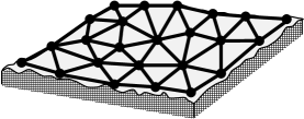
FIG. 1.: A randomly-tethered elastic membrane in contact with a disordered substrate.

We use an irregular array of beads tethered by harmonic springs to model the amorphous solid. Let the average inter-bead distance be $a$ and the equilibrium position of a bead labeled by $n$ be given by ${\bf R}_{n}\in\Re^{D}$. The neighboring beads are connected by harmonic springs with appropriately chosen spring lengths (of the order $a$) such that the configuration $\left\{{\bf R}_{n}\right\}$ is the unfrustrated ground state of the tethered system in the absence of any external forces.

To describe the large scale properties of such an elastic medium analytically, it will be useful to adopt a continuum description. Let the density field of the unperturbed system be

$$\rho_{0}({\bf r})=\sum_{\{n\}}\delta^{D}({\bf r}-{\bf R}_{n}).$$ (1)

The quenched-in density variation is $\delta\rho_{0}({\bf r})=\rho_{0}({\bf r})-\bar{\rho}$, where $\bar{\rho}\equiv a^{-D}$ is the average density; it is characterized by the correlation function

$$\overline{\delta\rho_{0}({\bf r})\delta\rho_{0}({\bf r^{\prime}})}\equiv C_{0}({\bf r}-{\bf r^{\prime}}),$$ (2)

or the structure factor $S_{0}({\bf k})=\int d^{D}{\bf r}\,C_{0}({\bf r})e^{i{\bf k}{\bf r}}$. Here the overbar denotes average over the ensembles of quenched bead positions $\{{\bf R}_{n}\}$. In the case of a single large system, the overbar can be taken as the spatial average over smaller subsystems.

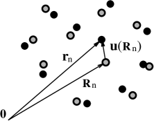
FIG. 2.: The equilibrium position (circle) of a bead $n$ is given ${\bf R}_{n}$; the actual position (black dot) ${\bf r}_{n}$ is given by the displacement vector ${\bf u}({\bf R}_{n})$. Note that the set $\{{\bf R}_{n}\}$ is not necessarily ordered periodically.

Elastic distortion of the discrete system is described by a displacement vector ${\bf u}({\bf R}_{n})$, which denotes the displacement of the $n^{{\rm th}}$ bead from its equilibrium position ${\bf R}_{n}$; see Fig. 2. Then the actual position of the bead is ${\bf r}_{n}={\bf R}_{n}+{\bf u}({\bf R}_{n})$, and the corresponding density field is

$$\rho({\bf r};{\bf u}) = \sum_{\{n\}}\delta^{D}\big{(}{\bf r}-{\bf R}_{n}-{\bf u}({\bf R}_{n})\big{)}$$ (3)

$$\approx (1-\mbox{\boldmath$\nabla$}\cdot{\bf u})\sum_{\{n\}}\delta^{D}\big{(}{\bf r}-{\bf R}_{n}-{\bf u}({\bf r})\big{)},$$ (4)

where we assumed that variations in the displacement is small, i.e., $\mbox{\boldmath$\nabla$}\cdot{\bf u}\ll 1$. Comparing Eq. (4) with Eq. (1), we see that

$$\rho({\bf r},{\bf u}) = (1-\mbox{\boldmath$\nabla$}\cdot{\bf u})\cdot\rho_{0}({\bf r}-{\bf u})$$ (5)

$$\approx \bar{\rho}(1-\mbox{\boldmath$\nabla$}\cdot{\bf u})+\delta\rho_{0}({\bf r}-{\bf u})$$ (6)

to leading order in $(\mbox{\boldmath$\nabla$}\cdot{\bf u})$. In the continuum description, details of the elastic medium are contained completely in the term $\delta\rho_{0}({\bf r})$, through the correlation function $C_{0}({\bf r})$.

In the absence of any external forces, the energy of the tethered system is invariant upon a constant displacement ${\bf u}\to{\bf u}+const$. For a statistically isotropic medium, the energy of small elastic distortion is then simply given by the classical form [58]

$${\cal H}_{0}=\int d^{D}{\bf r}\left\{\frac{c_{11}}{2}(\mbox{\boldmath$\nabla$}\cdot{\bf u})^{2}+\frac{c_{66}}{2}(\mbox{\boldmath$\nabla$}\times{\bf u})^{2}\right\},$$ (7)

where $c_{11}$ and $c_{66}$ are the bulk and shear elastic moduli [59].

Consider now the situation where the elastic medium is in contact with a disordered substrate, modeled by a Gaussian random potential $V({\bf r})$ with zero mean and a variance

$$\left[V({\bf r})V({\bf r^{\prime}})\right]=\Delta_{V}\,\delta^{D}({\bf r}-{\bf r}^{\prime}).$$ (8)

Here, $\left[...\right]$ denotes average over the ensemble of substrates. The interaction of the medium with the substrate is described by a pinning energy,

$${\cal H}_{{\rm pin}} = \sum_{\{n\}}V({\bf r}_{n})=\int d^{D}{\bf r}\,\rho({\bf r},{\bf u})V({\bf r})$$ (9)

$$= \int d^{D}{\bf r}\,\Big{\{}-\bar{\rho}(\mbox{\boldmath$\nabla$}\cdot{\bf u})V({\bf r})+W({\bf r},{\bf u}({\bf r}))\Big{\}},$$ (10)

where

$$W({\bf r},{\bf u})\equiv\delta\rho_{0}({\bf r}-{\bf u})V({\bf r}),$$ (11)

and the term $\bar{\rho}V({\bf r})$ is neglected as it produces merely an overall energy shift. Note that $W({\bf r},{\bf u})$ depends explicitly on ${\bf u}$ where as other terms depend only on $\mbox{\boldmath$\nabla$}\,{\bf u}$. Thus, only $W$ breaks the translational symmetry ${\bf u}\to{\bf u}+const$, and is responsible for providing the pinning phenomenon. The interacting system, characterized by the effective Hamiltonian

$${\cal H}={\cal H}_{0}+\int d^{D}{\bf r}\,\Big{\{}-\bar{\rho}\,(\mbox{\boldmath$\nabla$}\cdot{\bf u})V({\bf r})+W({\bf r},{\bf u})\Big{\}},$$ (12)

will be analyzed in detail in the next section [60].

III Thermodynamic Properties

A Theoretical Considerations

1 The Periodic Medium

If the tethered system does not contain any quenched-in defects, then the intrinsic density variation is periodic, i.e.,

$$\delta\rho_{0}({\bf x})\sim\overline{\rho}\,\sum_{i}\cos\left({\bf K}_{i}\cdot{\bf x}\right),$$ (13)

where ${\bf K}_{i}$’s are the reciprocal lattice vectors. Eq. (12) in this case reads

$${\cal H}_{{\rm CDW}} = {\cal H}_{0}+\int d^{D}{\bf r}\Big{\{}-\bar{\rho}\,(\mbox{\boldmath$\nabla$}\cdot{\bf u})V({\bf r})$$ (15)

$$\quad+\sum_{i}\bar{\rho}\,V({\bf r})\,\cos\big{[}{\bf K}_{i}\cdot{\bf(r-u(r)}\big{]}\Big{\}}.$$

The model (15) is the $D$-component generalization of the randomly-pinned charge-density wave (CDW) in $D$-dimensions [61, 62]. The equilibrium properties of this class of systems have been well studied [10, 11, 13]: It is known that the disorder is irrelevant in $D=1$, where the system behaves like a Gaussian chain. In $D>2$, the system (15) is glassy at any finite temperatures [11, 13]. The glass phase is described by two critical exponents: the thermal exponent $\theta$ characterizing typical fluctuations of the free energy landscape $\Delta{\cal F}\sim L^{\theta}$ for elastic distortion over the length scales $L\gg a$, and the “wandering” exponent $\zeta$ characterizing fluctuations of the displacement field, $\Delta u\sim L^{\zeta},$ in the low free energy state(s). The results $\theta=D-2$ and $\zeta=O(\log)$ is believed to be exact for $2<D\leq 4$. Right in $D=2$, the situation is somewhat more complicated [10, 63, 64]. The disorder is irrelevant for $T>T_{g}\propto\left(\bar{\rho}\,\big{(}c_{11}^{-1}+c_{66}^{-1}\big{)}\right)^{-1}$. The precise value of the glass temperature $T_{g}$ depends on the microscopic model [61, 62]. Below $T_{g},$ the 2-dimensional system is in a “marginal” glass phase [10, 61, 62, 65] characterized by logarithmic anomalies in $\Delta{\cal F}$ and $\Delta u$.

2 Strongly-disordered Medium

If the tethered system contains a finite concentration of quenched-in dislocations and/or disclinations, then the density variation $\delta\rho_{0}$ is no longer described by (13), and one must characterize $\delta\rho_{0}$ statistically through the correlation function $C_{0}({\bf r})$ or the structure factor $S_{0}({\bf k})$. Consider the simpler case where $S_{0}({\bf k})$ is liquid-like, containing no Bragg peaks at finite ${\bf k}$. This may describe, for example, a completely disordered film such as a rubber sheet, or a randomly-polymerized liquid membrane. The model defined by Eqs. (11) and (12) now contains two kinds of (mutually uncorrelated) disorders in the effective random potential $W({\bf r},{\bf u})$, making it difficult to solve systematically. In fact, straightforward application of the replica trick to the model (12) immediately leads to difficulties as one has to integrate out the disorders twice.

However, if we simply treat $W({\bf r},{\bf u})$ as an effective disorder and examine its moments using (2) and (8), we find it has zero mean and a variance given by

$$\overline{[W({\bf r},{\bf u})W({\bf r}^{\prime},{\bf u}^{\prime})]} = \Delta_{V}\delta^{D}({\bf r}-{\bf r}^{\prime})\,C_{0}({\bf u}-{\bf u}^{\prime})$$ (16)

$$\approx \Delta\,\delta^{D}({\bf r}-{\bf r}^{\prime})\,\delta^{D}({\bf u}-{\bf u}^{\prime}),$$ (17)

with $\Delta=\Delta_{V}S_{0}({\bf k}\to 0)$ for short-range correlated function $C_{0}({\bf r})$.

Note that the form of the correlator (17) is the same as that of an uncorrelated random potential in the space $({\bf r},{\bf u})\in\Re^{D+D}$. It is then tempting to interpret the system (12) as a $D$-component, $D$-dimensional “directed manifold” ${\bf u}({\bf r})$ embedded in an effective $(D+D)$-dimensional random potential $W({\bf r},{\bf u})$. The latter is an example of the so-called “random manifold” problem which is encountered in a wide variety of context involving quenched randomness [6, 14, 66, 67]. Properties of the random manifold (RM) have been characterized in detail and are briefly summarized here: It is known that an $d$-component RM in $D$-dimension is asymptotically described by a glass phase at any finite temperatures if

$$2D>d\,(2-D).$$ (18)

Outside this regime, the glass phase is still obtained if the temperature is below a certain critical temperature [68] $T>0$. Like the randomly pinned CDW, the behavior of the RM in the glass phase can be described by the thermal exponent $\theta$ and wandering exponent $\zeta$. There is an exact exponent identity $\theta=D-2+2\zeta$ linking the two exponents for all $d$ and $D$. The exponents are known exactly for the special case [17] $D=1$ and $d=1$, with $\zeta=2/3$ and $\theta=1/3$. There are also strong bounds on the exponents, with $(4-D)/4\leq\zeta\leq\max\left\{(4-D)/(4+d),(2-D)/2\right\}$. [Note that $\zeta\rightarrow 0$ as $D\rightarrow 4^{-}$, reflecting the fact that $D=4$ is the upper critical dimension of the problem.] Numerically, the exponents for various $d$ and $D$ have been determined to good accuracy [17, 18]. The results are approximately summarized by the expression

$$\zeta\approx\frac{2(4-D)}{8+d}$$ (19)

which was motivated by a functional renormalization-group consideration [66].

What does the random manifold problem have to do with the problem at hand ? Even though the second moment of $W({\bf r},{\bf u})$ is of the same form as that of a $(D+D)$-dimensional random potential, $W$ itself, being the product of two $D$-dimensional random functions, certainly cannot be truly be a short-range correlated $(D+D)$-dimensional random potential. There must be long-range correlations, the forms of which are revealed by considering higher moments of $W$, for example, $W_{2}({\bf r},{\bf u})\equiv W^{2}({\bf r},{\bf u})-\overline{\left[W^{2}\right]}$. We find

$$\overline{\left[W_{2}({\bf r},{\bf u})W_{2}(0,0)\right]}=4\delta^{2}({\bf r})\delta^{2}({\bf u})+2\delta^{2}({\bf r})+2\delta^{2}({\bf r}-{\bf u}),$$ (20)

indicating correlations along the “directions” of constant ${\bf r}$ and constant ${\bf r}-{\bf u}$. Such correlations are of course not surprising given the form of $W({\bf r},{\bf u})$ in Eq. (11). Thus, a more accurate model of the effective random potential should include a superposition of short-range correlated and long-range correlated random potentials, e.g.,

$$W({\bf r},{\bf u})=W_{0}({\bf r},{\bf u})+W_{a}({\bf r})+W_{b}({\bf r}-{\bf u})$$ (21)

with $W_{0}({\bf r},{\bf u})$ being truly a short-ranged $(D+D)$-dimensional potential described by the correlator (17). The random potentials $W_{a}$ and $W_{b}$ generated from the higher moments of $W$ have the correlator $\overline{\left[W_{i}({\bf x})W_{j}({\bf x}^{\prime})\right]}\sim\delta_{ij}\delta({\bf x}-{\bf x}^{\prime})$.

Clearly, $W_{a}({\bf r})$ has no effect on the behavior of the system as it does not involve ${\bf u}$. Since $|{\bf u}|\ll|{\bf r}|$ ($\zeta<1$), the ${\bf u}$-dependence in $W_{b}({\bf r}-{\bf u})$ is perturbatively irrelevant, and we conclude that $W_{b}$ does not play a significant role either in the limit of weak disorders. Another way to gain some intuition of the correlated potential is through an example in $D=1$. In Fig. 3, we illustrate the form of the effective random potential (21) in $D=1$, where the “random manifold” is usually referred to as a “directed path” (directed horizontally in the direction $r$ of Fig. 3), and the correlated potentials are like the “columnar defects” encountered in the pinning of flux lines in high-$T_{c}$ superconductors [69, 70, 71, 72]. These columnar defects are known to be strongly relevant if oriented in the direction of the directed path (the $r$-direction in Fig. 3). However, they are irrelevant if tilted away by a slope exceeding a finite threshold given by the strength of the disorder. The correlated potentials $W_{a}$ and $W_{b}$ are just the $D$-dimensional generalization of the “tilted” columnar defects. Their irrelevance can be established more rigorously by extending, for example, the analysis of Ref. [70] to $D$-dimensions and will not be pursued here.

FIG. 3.: Schematic illustration of the effective random potential (21) in $D=1$, for a path directed in the horizontal $r$-direction: The correlated component is shown as two sets of “columnar defects”, pointing along the directions $r={\rm const}$ and $r-u={\rm const}$; the uncorrelated component is shown as “point defects”.

For strong disorders, a large distortion with ${\bf u}\sim{\bf r}$ is admissable by our model defined by Eqs. (12) and (11): Such a distortion would be favorable if the elastic energy cost (per volume) is more than compensated by the disorder energy gained. The latter is given by the order of variations in $W_{b}$ and is finite. Thus, our model can in principle display a phase transition to a “localized phase” where ${\bf u}\sim{\bf r}$, similar to what was found by Hatano and Nelson in the context of non-Hermitian quantum mechanics [72]. However, the formation of this localized phase would require different “beads” of the manifold all to lie with a finite volume of the substrate. This is clearly unphysical and is prevented in practice by any excluded-volume interaction between the beads.

Based on the above analysis, we conjecture that the long-ranged correlations in $W({\bf r},{\bf u})$ are irrelevant for arbitrary disorder strengths, and the problem of a random elastic medium on a disordered substrate belongs to the same universality class as that of the random manifold with $d=D$ [73, 74]. Since the condition (18) is always satisfied for $d=D$, we expect our system to be glassy at all finite temperatures, with the exponents

$$\zeta\approx\frac{2(4-D)}{8+D}\qquad{\rm and}\qquad\theta\approx\frac{D(2+D)}{8+D}$$ (22)

upon adopting the approximate formula (19).

Our conjecture was presented for the case $D=1$ previously in a short communication [51]. In Sec. III.B below, we present results of an extensive numerical study. We find that all universal aspects of the $D=1$ problem measured, including amplitude ratios, agree quantitatively with those of the 1+1 dimensional directed path in random media, thus verifying our conjecture for $D=1$. Very recently, Zeng et al [75] applied the min-cut-max-flow algorithm [18, 19] to investigate the $D=2$ version of the model defined by (11) and (12), but with only one component of the displacement field ${\bf u}$. They found an exponent value $\zeta\approx 0.42$, which is consistent with that of the random manifold with $d=1$ and $D=2$ ($\zeta=0.41\pm 0.01$), as expected according to our conjecture. For a 2-dimensional random elastic medium on a 2-dimensional substrate, we predict that $\zeta\approx 0.4$ and $\theta\approx 0.8$ as for a $2$-component, $2$-dimensional directed manifold in $4$-dimensional random medium. An entangled flux line array, e.g., a “polymer glass”, may be modeled [76] by a 2-component, 3-dimensional random elastic system for time scales up to the distanglement time $\tau\sim e^{U_{\times}/T}$, where $U_{\times}$ is the flux cutting energy estimated to be of the order of $10$ times the melting temperature [77]. The corresponding exponents are thus expected to be $\zeta\approx 0.2$ and $\theta\approx 1.4$ in the elastic regime.

3 Nearly-periodic Medium

We next turn to the case of a nearly-periodic, tethered system with a low concentration of quenched-in defects. This could be the case of a rigid vortex array on a thin film superconductor, the defects being frozen-in vacancies and interstitials [54]. Since a low density of vacancies/interstitials does not destroy the crystallinity of the elastic system, Bragg peaks in $S_{0}({\bf k})$ still leads to a CDW-type interaction (15) when the elastic medium is placed in contact with the disordered substrate. However, the presence of quenched-in vacancies and interstitials also gives rise to large-scale density variations, manifested by a nonzero component of $S_{0}({\bf k}\rightarrow 0)$, which leads to the effective $(D+D)$-dimensional random potential as described by the correlator (17). Thus, the nearly-periodic elastic system is subject to both the CDW-type and the RM-type disorders. What is the outcome of competition between these two kinds of interactions ? A simple power counting reinforces the intuitively obvious result that the RM interaction is relevant in the CDW phase, while the CDW interaction is not relevant in the RM phase. We thereby conclude that even the nearly-periodic elastic system belongs to the RM universality class.

Our analysis indicates that any finite concentration of quenched-in defects is sufficient to change the CDW-type pinning of a perfectly periodic system to the much stronger pinning of the random-manifold universality class. This includes a low concentration of quenched-in interstitials and vacancies, which by themselves do not destroy the crystallinity of the elastic medium. Such a result may be rather surprising at a first glance, since the existence of periodicity of an elastic medium is usually associated with the CDW universality class. But this notion is incorrect. What is responsible for the CDW universality class in the pinning of an usual periodic solid is a relabeling symmetry of the underlying discrete system, e.g., the energy of a configuration of beads described by $\left\{{\bf R}_{n}\right\}$ is the same as that described by $\left\{{\bf R}_{n+{\rm const}}\right\}$ (up to boundary effects). This relabeling symmetry is broken [78] given a finite concentration of interstitials/vacancies, since different beads are no longer equivalent. Thus, asymptotically, the system is controlled by the RM fixed point.

Lastly, we mention that even if the medium contains no topological defects at all (not even interstitials and vacancies), some quenched-in “phonon modes” may already be sufficient to induce the RM behavior: Let the equilibrium positions of the beads labeled by $(n_{1},n_{2})$ be ${\bf R}_{n_{1},n_{2}}={\cal R}_{n_{1},n_{2}}+{\bf w}_{n_{1},n_{2}}$, where ${\cal R}_{n_{1},n_{2}}$ denotes the points of a periodic lattice, and ${\bf w}$ is the quenched-in phonon modes characterized by $[({\bf w}({\bf x})-{\bf w}({\bf x}^{\prime}))^{2}]=\Delta({\bf x}-{\bf x}^{\prime})$. Then the correlator of the effective pinning energy $W$ is [79]

$\displaystyle\overline{[W({\bf r},{\bf u})W(0,0)]}=\Delta_{V}\,\delta^{D}({\bf r})\sum_{i}\cos({\bf K}_{i}\cdot{\bf u})e^{-\frac{\Delta({\bf u})}{2{\bf K}_{i}^{2}}},$

where ${\bf K}_{i}$’s are again the reciprocal lattice vectors. Since $\overline{[W({\bf r},{\bf u})W(0,0)]}$ is short-ranged correlated in ${\bf u}$ as long as $\Delta({\bf u})$ diverges for large $|{\bf u}|$ (including logarithmic divergence), we see that the RM universality class is recovered even for quenched-in phonon fluctuations in $D\leq 2$.

B Transfer Matrix Studies

We test our predictions by performing numerical studies of a one-dimensional bead-spring system corresponding to the $D=1$ case of the randomly-tethered elastic medium considered above. The one dimensional system is chosen since its thermodynamic properties can be obtained in polynomial ($N^{2}$) time using the transfer matrix method [16], and also the thermodynamics of the corresponding $(1+1)$-dimensional problem of a directed path in random media (DPRM) is known exactly [17]. Thus a quantitative comparison can be made.

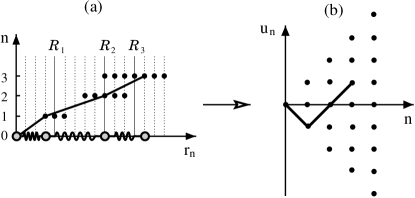
FIG. 4.: Longitudinal displacement variation of the beads of the random chain in (a) is represented as a directed path on a $(1+1)$-dimensional lattice in (b). The equilibrium spring lengths are $a_{1}=4$, $a_{2}=5$, and $a_{3}=3$. The equilibrium positions $R_{n}=\sum_{m=1}^{n}a_{m}$ are indicated in (a) as solid lines. The open circles indicate the allowed bead positions, given the SOS-like restriction on $u_{n}$.

We consider the following discretized one-dimensional problem: A chain of $N+1$ beads (labeled sequentially by $n\in[0,N]$) is placed on a one-dimensional lattice of unit lattice spacing. Each bead $n$ (except for $n=0$) is connected to its nearest neighbor $n-1$ by a harmonic spring. All springs have the same spring constant $\gamma$, but the equilibrium length $a_{n}$ is an integer drawn randomly from the interval $[5,15]$ (in units of the lattice spacing), such that the mean spring length is $a=10$. The equilibrium positions of the $n^{{\rm th}}$ bead is $R_{n}=\sum_{m=1}^{n}a_{m}$ if we fix the $n=0$ end of the chain at the origin. To speed up the numerics, we apply an SOS-like restriction and allow the springs to be compressed or stretched by at most one lattice unit. (We have verified that allowing for large excitations does not affect scaling properties of a long chain.) Then the chain configuration is given by the position of each bead $n$

$$r_{n}=R_{n}+u_{n},$$ (23)

where $u_{n}\in\{0,\pm 1,\pm 2,\ldots\;,\pm n\}$ is the “displacement field”, with the restriction $(u_{n+1}-u_{n})\in\{0,\pm 1\}$, and the energy of each spring is $\frac{\gamma}{2}(u_{n+1}-u_{n})^{2}=\left\{0,\pm\frac{\gamma}{2}\right\}$. Since each chain configuration is uniquely specified by the set of numbers $\{u_{n}\}=(u_{1},u_{2},\ldots,u_{N})$, we may represent the chain as a directed path in $1+1$-dimensions, with “transverse” coordinate $\{u_{n}\}$. The mapping is illustrated in Fig. 4. The allowed bead positions are marked by open circles in Fig. 4(a) and shifted upwards for clarity. The chain with $N+1$ beads has a total of $3^{N}$ different configurations. One of these configuration with $\{u_{n}\}=(-1,0,1)$ (as shown in Fig. 4(a)) is represented by the full line in the directed path representation of Fig. 4(b).

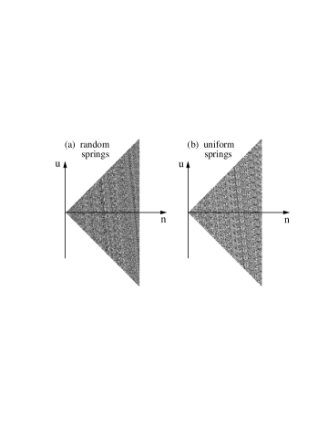
FIG. 5.: Gray-scale plots of potential $W_{n}(u)=V(R_{n}+u)$, $R_{n}=\sum_{m=1}^{n}a_{m}$, for a chain with $N=100$ elements. (a) Random springs with $a_{n}$ uniformly distributed in interval $[5,15]$, and (b) uniform springs with $a_{n}=10$. Lighter shades correspond to larger values of $W$.

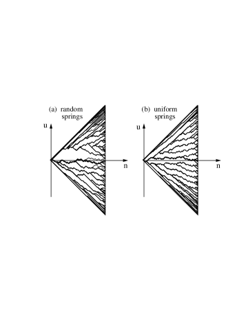
FIG. 6.: Collection of the locally optimal paths for disorder potential $W$ shown in Figs. 5(a) and (b). The bold lines represent the global optimal paths.

Next, we specify the energetics of the system. Disorder of the substrate with which the chain is in contact is given by the function $V(r)$, drawn independently from a Gaussian distribution of zero mean and unit variance for each lattice point $r$. The spring constant used is $\gamma=0.2$ such that the typical “spring energy” is $0.1$, much smaller than the disordered “potential energy” $\sim O(1)$. This choice of parameters facilitates a quick approach to the asymptotic (glassy) regime. In term of the displacement variable $u_{n}$, the random potential can be written as $W_{n}(u_{n})\equiv V(R_{n}+u_{n})$, which depends explicitly on the two sources of randomness, $V(r)$ and $R_{n}$. It is illustrative to plot $W_{n}(u)$ in the two dimensional space $(n,u)$ (Fig. 5(a)). For comparison, the case of uniform springs (with $a_{n}=10$ for all $n$’s) is shown in Fig. 5(b). We see that the periodic feature of $W$ shown in Fig. 5(b) is randomized by the random springs. However, correlations in a slanted direction is still clearly visible in Fig. 5(a) (cf. Fig. 3).

Effect of the different potential $W$ on the directed path can be illustrated by differences in the morphology of the “local optimal paths”, i.e., the collection of the lowest energy paths [16, 17] of length $N$, connecting the starting point at the origin and all possible ending points at $(N,u)$. In Figs. 6(a) and (b), we plot the optimal paths for the realizations of $W$ shown in Figs. 5(a) and (b) respectively. The bold line corresponds to the global optimal path, the lowest energy path among all the local optimal paths. Note that the local optimal paths of the system with uniform springs (Fig. 6(b)) are very regularly arranged, with the distance between neighboring branches almost constant and approximately equal to the equilibrium spring length $a$. On the other hand, the local optimal paths for the random chain are arranged much more irregularly (Fig. 6(a)). There are for example large islands of high energy regions which the paths avoid, similar to what was found previously for the directed path in 2-dimensional random potential [16, 17]. Thus, we can view these paths configurations as an indication of possible equivalence between the statistical properties of a random chain on one-dimensional random substrate and a directed path in 2-dimensional random medium.

The statistics of the optimal paths have been investigated in Ref. [51], where we presented numerical results obtained from the zero-temperature transfer matrix solution of systems with $N=4096$, averaged over $2000$ independent realizations of $V(r)$ and $\{a_{n}\}$ pairs. Fluctuations in the end-to-end displacement $u_{N}^{*}$ and the total energy $E^{*}(N)$ of the global optimal path $\{u_{n}^{*}\}$ indicate scaling behavior with $\overline{[(u_{N}^{*})^{2}]}\sim\overline{[u_{N}^{*}]}^{2}\sim N^{4/3}$ and $\overline{[(E_{N}^{*})^{2}]}-\overline{[E_{N}^{*}]}^{2}\sim N^{2/3}$, both of which are characteristic of the 1+1 dimensional DPRM universality class [17]. Here, we describe extension of the zero-temperature calculations to finite temperatures.

FIG. 7.: Log-log plot of the sample-to-sample free energy fluctuation $(\Delta{\cal F})^{2}(N)$ for various chain lengths $N$. Thin straight line shows the predicted asymptotic scaling.

FIG. 8.: Log-log plot of the end-to-end displacement fluctuations for different chain length $N$, at the temperature $T=1$. Also shown is the connected thermal fluctuation $\delta u_{N}^{2}$.

The Boltzmann weight ${\cal W}_{N}(u)$ for paths connecting their origin at $(0,0)$ to their end points at $(N,u)$ can be obtained recursively according to [16, 80]:

$${\cal W}_{n+1}(u) = c_{0}(n,u){\cal W}_{n}(u)$$ (25)

$$+c_{1}(n,u)\Big{\{}{\cal W}_{n}(u-1)+{\cal W}_{n}(u+1)\Big{\}},$$

where $c_{0}(n,u)=e^{W_{n}(u)/T}$, $c_{1}(n,u)=c_{0}(n,u)\,e^{-\gamma/(2T)}$, with the “initial condition” ${\cal W}_{0}(u)=\delta_{u,0}$. The partition function ${\cal Z}_{n}$ is obtained as ${\cal Z}_{n}=\sum_{u}{\cal W}_{n}(u)$, and the free energy is ${\cal F}_{n}=-T\ln{\cal Z}_{n}$. The thermal averaging of an observable ${\cal O}_{n}(u)$ is given by

$$\langle{\cal O}_{n}\rangle\equiv\frac{\sum_{u}{\cal O}_{n}(u){\cal W}_{n}(u)}{\sum_{u}{\cal W}_{n}(u)}.$$ (26)

The sample-to-sample free energy fluctuation $(\Delta{\cal F})^{2}=\overline{[{\cal F}_{N}^{2}]}-\overline{[{\cal F}_{N}]}^{2}$ is shown in Fig. 7. The results are obtained at temperature $T=1.0$, from systems with $N=1024$ averaged over 4000 different realizations of random $V(r)$ and $\{a_{n}\}$. It is seen that $(\Delta{\cal F})^{2}(N)$ approaches the asymptotic scaling form $N^{2/3}$. We also computed the finite-temperature end-to-end displacement fluctuations $\overline{[\langle u_{N}^{2}\rangle]}$ and $\overline{[\langle u_{N}\rangle^{2}]}$. As shown in Fig. 8, the approach to the expected $N^{4/3}$ behavior is clear. More interestingly, note that the disorder average of the thermal fluctuation itself, i.e., the connected second moment $\delta u_{N}^{2}\equiv\overline{[\langle u_{N}^{2}\rangle-\langle u_{N}\rangle^{2}]}$ in fact scales as $N^{1}$ as if randomness is not present. This behavior is expected of the DPRM due to a statistical tilt symmetry [17, 81, 82]. Such a symmetry is obviously not present in the bare potential $W_{n}(u)$ shown in Fig. 5(a). The scaling law on $\delta u_{N}^{2}$ found is therefore another evidence indicating the irrelevancy of the slanted correlation in $W_{n}(u)$ and the dominance of the 1+1 dimensional DPRM behavior.

FIG. 9.: Log-log plot of $g_{N}(T)$ as a function of temperature, averaged over $10^{5}$ different realizations of disorder. The high temperature behavior approaches $1/T^{2}$, which is expected of the $1+1$ dimensional DPRM.

FIG. 10.: Probability distribution for the free energy, plotted for the rescaled variable, $\delta{\cal F}=\left({\cal F}-\overline{[{\cal F}]}\right)/\Delta{\cal F}(N)$, at $T=1.0$ for system sizes ranging from $N=32$ to $N=1024$. Data were collected from $4096$ samples.

Our results suggest that the finite temperature behavior of the system probed is dominated by the $T=0$ fixed point. This result is not immediately generalizable to all $T$. Naively, one might think that at sufficiently high $T$ such that the thermal fluctuation $\delta u_{N}$ exceeds the quenched variation in $R_{N}$, then the effect of random spring length may be washed out. To investigate the possible existence of a finite temperature phase transition, we compute the dimensionless quantity [83]

$$g_{N}(T)=\overline{[\langle u_{N}\rangle^{2}]}\left/\overline{[\langle u_{N}^{2}\rangle]}\right.,$$ (27)

which vanishes for $T\rightarrow\infty$ while $g\rightarrow O(1)$ for $T\rightarrow 0$. If there is a phase transition at some finite temperature $T_{c}$, the expected finite-size scaling in the critical region would be $g_{N}(T)=\widetilde{g}\big{(}N^{1/\nu}(T-T_{c})\big{)}$, where $\nu$ is the correlation length exponent. Therefore, the curves of $g(T)$ for different $N$’s should all intersect each other at $T_{c}$ if a finite temperature transition exists. The numerical data for $g_{N}(T)$ in the temperature range $T=0.1$ to $3.0$, for system sizes from $N=4$ to $N=128$ are shown in Fig. 9. No indication of curve crossing at $T>0$ is found. In fact, the high temperature behavior of $g_{N}(T)$ approaches $1/T^{2}$ similar to that of the $(1+1)$-dimensional DPRM which has no finite temperature phase transition [83]. We therefore conclude that in the thermodynamic limit $N\rightarrow\infty$, there is no finite temperature phase transition, and the large scale behavior of the random chain is always described by the zero-temperature (glassy) system.

We have also calculated the full free energy probability distribution $P$ for different lengths $N$. Figure 10 shows data collapse of $P_{N}(\delta{\cal F})$ for $N=32$ to $N=1024$, collected from 4096 samples, with $\delta{\cal F}\equiv({\cal F}-\overline{[{\cal F}]})/\Delta{\cal F}(N)$ being the dimensionless measure of free energy variation. The distribution is asymmetric. The skewness $\gamma_{3}$ and kurtosis $\gamma_{4}$ of this distribution are plotted in Fig. 11(a) and Fig. 11(b) respectively for different $N$’s. Both $\gamma_{3}$ and $\gamma_{4}$ are found to approach the corresponding universal numbers (dashed lines) known for the (1+1)-dimensional DPRM [83]: $\gamma_{3}=-0.296\pm 0.028$, $\gamma_{4}=3.16$.

Putting together all the numerical results presented in this section, we see strong evidence supporting our expectation that the thermodynamics of a random chain on the disordered substrate and the (1+1)-dimensional DPRM indeed belong to the same universality class.

FIG. 11.: Skewness $\gamma_{3}$ and kurtosis $\gamma_{4}$ of the free energy distribution for different chain lengths $N$. Dashed lines are the corresponding values for the $(1+1)$-dimensional DPRM: $\gamma_{3}\approx-0.296$ and $\gamma_{4}\approx 3.16$.

IV Driven Dynamics

A Theoretical Considerations

1 Driven CDW and Random Manifolds

The zero-temperature driven dynamics of the tethered system is of interest to the study of tribology and to understanding the nonequilibrium dynamics of vortices. From the correspondence between the thermodynamic properties of the randomly-tethered elastic system and the CDW/RM systems, it is tempting to conjecture that the correspondence persists also for the dynamical properties. Before we provide evidences in support of this generalization, let us first review the known dynamics of the driven CDW/RM systems.

Consider first the simplest zero-temperature driven dynamics of the randomly-pinned (one-component) CDW in $D$-dimension [4, 5], given by the equation of motion

$$\mu_{0}^{-1}\partial_{t}u({\bf r},t)=-\frac{\delta}{\delta u}{\cal H}_{{\rm CDW}}\{u\}+F$$ (28)

where $\mu_{0}$ is a bare frictional coefficient, and $F$ is the driving force. For $F$ below some threshold force $F_{c}$, the average velocity $v\equiv\left\langle\partial_{t}u\right\rangle$ is zero. [Here, $\left\langle...\right\rangle$ denotes temporal and spatial average.] Upon approaching the threshold from below, the dynamics (e.g., response to perturbation) becomes very “jerky”. It is consisted of a series of “avalanches”, whose (linear) size $\ell$ obeys a power-law distribution [49],

$$\Pr(\ell>s)=s^{-\kappa}\,\widehat{\rho}(s/\xi).$$ (29)

In Eq. (29), $\xi$ is the correlation length of the system, $\widehat{\rho}(x)$ is a scaling function which is constant for $x\ll 1$ and drops off sharply for $x\gg 1$. The correlation length diverges as $\xi\sim(F_{c}-F)^{-\nu}$ as $F\rightarrow F_{c}^{-}$. The motion becomes continuous for $F>F_{c}$ due to overlapping avalanches. There the interface acquires a finite velocity with $v\sim(F-F_{c})^{\beta}$, similar to the emergence of the order parameter in a critical phenomenon. These exponents have been computed by a functional renormalization group (FRG) analysis [5] to first order in $\epsilon=4-D$, with $\nu=1/2$ and $\beta=1-\epsilon/6$. The one-loop FRG results are found to be consistent with extensive numerical simulations of the driven CDW in various spatial dimensions [23, 24, 25]. For example, Myers and Sethna [25] find the one-dimensional driven CDW ($\epsilon=3$) to have $\nu\approx 0.4\pm 0.1$ and $\beta\approx 0.45\pm 0.05$.

Similar depinning phenomenon [2] is obtained for the zero-temperature driven dynamics of the $d$-component random manifold ${\bf u}({\bf r)}$, whose equation of motion is

$$\mu_{0}^{-1}\partial_{t}{\bf u}({\bf r},t)=-\frac{\delta}{\delta{\bf u}}{\cal H}_{{\rm RM}}\left\{{\bf u}\right\}+{\bf F},$$ (30)

where ${\cal H}_{{\rm RM}}$ refers the random manifold Hamiltonian (12) with a truly random $(d+D)$-dimensional potential $W$, and ${\bf F}$ is again the driving force. A continuous depinning transition occurs at a critical force $\left|{\bf F}\right|=F_{c}$, where the system exhibits avalanches with power-law distribution as in (29). In the vicinity of the critical point, the exponents $\nu$ and $\beta$ can be defined as before. [Here, $\beta$ is the exponent describing the onset of the parallel component of the velocity, $v\equiv\left\langle\partial_{t}{\bf u}\right\rangle\cdot{\bf\hat{F}}$.] As the driving force ${\bf F}$ breaks the isotropy of the system, it is convenient [22] to divide the displacement ${\bf u}$ into components parallel and perpendicular to ${\bf F}$, with $u_{\parallel}\equiv{\bf u}\cdot{\bf\hat{F}}$ and ${\bf u}_{\perp}\equiv{\bf u}-u_{\parallel}\,{\bf\hat{F}}$. The depinning transition can then be understood in terms of the critical fluctuations in $u_{\parallel}$ and ${\bf u}_{\perp}$, given by the correlation functions

$$\left\langle\big{(}u_{\parallel}({\bf r},t)-u_{\parallel}({\bf 0},0)\big{)}^{2}\right\rangle = |{\bf r}|^{2\chi_{\parallel}}\,\hat{g}_{\parallel}(|t|/|{\bf r}|^{z_{\parallel}})$$ (31)

$$\left\langle\big{(}{\bf u}_{\perp}({\bf r},t)-{\bf u}_{\perp}({\bf 0},0)\big{)}^{2}\right\rangle = |{\bf r}|^{2\chi_{\perp}}\,\widehat{g}_{\perp}(|t|/|{\bf r}|^{z_{\perp}})$$ (32)

at $\left|{\bf F}\right|=F_{c}$. They are characterized by their respective roughness exponent $\chi_{\parallel,\perp}$ and dynamic exponent $z_{\parallel,\perp}$, from which all other exponents can be obtained [2]. For example, $\nu=1/(2-\chi_{\parallel})$, $\beta=\nu\,(z_{\parallel}-\chi_{\parallel})$ and $\kappa=D-2+\chi_{\parallel}$ [84]. It was shown by Ertas and Kardar [22] that the scaling properties of $u_{\parallel}$ are the same as those of the one-component system (RM with $d=1$) which has been solved by the FRG method [20, 21], with $\chi_{\parallel}=\epsilon/3$ and $z_{\parallel}=2-2\epsilon/9$ to first order in $\epsilon=4-D$. Ertas and Kardar also found [22] $\chi_{\perp}=\chi_{\parallel}-\frac{D}{2}$ and $z_{\perp}=z_{\parallel}+\nu^{-1}$.

Numerically, one finds for the one-dimensional interface in (1+1)-dimensions [27] (i.e, $d=D=1$ or $\epsilon=3$) that $\chi\approx 0.97\pm 0.05$, $\nu\approx 1.05\pm 0.1$, and $\beta\approx 0.24\pm 0.1$. For the two-dimensional interface in 3-dimensions [85] ($d=1$ and $\epsilon=2$), the exponents are $\chi\approx 0.67\pm 0.03$ and $\nu\approx 0.75\pm 0.05$. These results are all consistent with the one-loop FRG predictions [20, 21]. In addition, a different exponent is found for the finite size scaling of the roughness [28], with

$$\langle\big{(}u(L,t)-u(0,t)\big{)}^{2}\rangle\sim L^{2\chi_{\rm FS}},$$

with $\chi_{{\rm FS}}\approx 1.25$ in $D=1$.

2 Driven Tethered Network

We now return to the randomly tethered elastic network defined in Sec. II, and study its motion in the presence of a uniform driving force ${\bf F}$ parallel to the substrate. We start with the deterministic and purely dissipative dynamics of the discrete bead-spring system. The equation of motion, in terms of the displacement vector ${\bf u}({\bf R}_{n})$ for the bead $n$, has the form

$$\mu_{0}^{-1}\partial_{t}{\bf u}({\bf R}_{n},t) = -\sum_{\{n^{\prime}\}}{\cal G}^{-1}({\bf R}_{n}-{\bf R}_{n^{\prime}})\cdot{\bf u}({\bf R}_{n^{\prime}},t)$$ (34)

$$-\frac{\delta}{\delta{\bf u}}V[{\bf R}_{n}+{\bf u}({\bf R}_{n},t)]+{\bf F},$$

where the kernel ${\cal G}^{-1}$ describes the spring forces exerted by all the beads $\{n^{\prime}\}$ connected with the bead $n$.

As we will show in Sec. IV.B, the behavior of this tethered network is very similar to that of the driven CDW and RM just described: At small driving forces the system is completely pinned by the random potential. As the force increases above some threshold value $F_{c}$, the system starts to move with a nonzero average velocity, $v\sim(F-F_{c})^{\beta}$. The behavior near the depinning transition is characterized by a diverging correlation length $\xi\gg a$ as in usual critical phenomena.

To study the depinning phenomenon, it is useful to coarse grain the equation of motion for the discrete system (34). The procedure is described in Appendix A for a 2D system. In term of the coarse-grained displacement field ${\bf u}$, the equation of motion becomes

$$\mu_{0}^{-1}\partial_{t}{\bf u}({\bf r},t)=(1-\mbox{\boldmath$\nabla$}\cdot{\bf u})\widetilde{{\bf f}}({\bf r},\{{\bf u}\})+{\bf f}_{\rm pin}({\bf r},{\bf u})$$ (35)

where

$$\widetilde{{\bf f}}({\bf r},\{{\bf u}\})=-\int_{{\bf r}^{\prime}}{\cal G}^{-1}({\bf r}-{\bf r^{\prime}})\cdot{\bf u}({\bf r}^{\prime},t)-\mbox{\boldmath$\nabla$}V_{<}({\bf r})+{\bf F}$$ (36)

results from the straightforward coarse graining of the right-hand side of Eq. (34), with $V_{<}({\bf r})$ being the slowly varying part of the substrate potential $V({\bf r})$. Since the beads in the tethered systems are connected only to other beads in their vicinities, the kernel ${\cal G}^{-1}$ is local. Its Fourier transform reads in component form

$$\widehat{G}_{ij}^{-1}\left({\bf k}\right)=c_{66}\delta_{ij}k^{2}+(c_{11}-c_{66})k_{i}k_{j},$$ (37)

where we have again neglected the spatial variations in the elastic moduli. Finally, the ${\bf u}$-dependent pinning force in (35) is

$${\bf f}_{\rm pin}({\bf r},{\bf u})=-\mbox{\boldmath$\nabla$}V_{>}({\bf r})\cdot\delta\rho_{0}({\bf r}-{\bf u})/\bar{\rho},$$ (38)

where $V_{>}({\bf r})$ are the Fourier modes of $V({\bf r})$ close to the inverse bead spacing.

For the system with uniform springs, density variation is given by (13). The equations of motion (35) – (38) are then similar to the ones describing the randomly-pinned ($D$-component) CDW. This is expected given the thermodynamic properties described in Sec. III. Compared to the “usual” equation of motion for the driven CDW, $\mu_{0}^{-1}\partial_{t}{\bf u}=-\delta{\cal H}_{\rm CDW}/\delta{\bf u}+{\bf F}$, Eqs. (35) – (38) contain addition terms such as $\mbox{\boldmath$\nabla$}V$ and $(\mbox{\boldmath$\nabla$}\cdot{\bf u})\,\widetilde{{\bf f}}$. These terms have recently been introduced on phenomenological grounds [86, 87]. Here we find that they can be obtained systematically [88] from a coarse-graining procedure (Appendix A). What effects do these additional terms have in the vicinity of the depinning transition ? The term $\mbox{\boldmath$\nabla$}V$ is ${\bf u}$-independent and hence does not provide pinning [89]. The term proportional to $(\mbox{\boldmath$\nabla$}\cdot{\bf u})$ is dynamic in origin. Kinetically-generated terms of this kind, including other terms with higher powers in $(\mbox{\boldmath$\nabla$}\cdot{\bf u})$, can drastically affect the behavior of the system in the limit of strong drive where $\widetilde{{\bf f}}$ is large. However, they are irrelevant in the vicinity of the depinning transition where $\partial_{t}{\bf u},\widetilde{{\bf f}}\to 0$ [90].

The introduction of random springs destroys periodicity in $\delta\rho_{0}$ and one must describe the random pinning force ${\bf f}_{\rm pin}({\bf r},{\bf u})$ statistically through the correlation function $C_{0}$ as done in the equilibrium case. We find

$$\overline{[f_{{\rm pin},i}({\bf r},{\bf u})f_{{\rm pin},j}(0,0)]} = \frac{\Delta_{V}}{\bar{\rho}^{2}}\,\left(\frac{2\pi}{a}\right)^{2}\delta_{ij}\,\delta({\bf r})C_{0}({\bf u}),$$ (39)

$$\approx \frac{\Delta_{V}}{\bar{\rho}^{2}}\delta({\bf r})\partial_{i}\partial_{j}C_{0}({\bf u})$$ (40)

which is short-range correlated in both ${\bf r}$ and ${\bf u}$ for short-ranged correlated $\delta\rho_{0}$. As in the static case analyzed in Sec. III, higher moments of ${\bf f}_{\rm pin}$ are long-range correlated but irrelevant. The critical dynamics with short-ranged pinning forces is then in the universality class of the driven RM [21]. In fact, the pinning force appears as if generated directly from the effective potential $W({\bf r},{\bf u})$, i.e., ${\bf f}_{\rm pin}\approx-\delta W({\bf r},{\bf u})/\delta{\bf u}$. We thus conjecture that the critical depinning dynamics of the $D$-dimensional randomly-tethered elastic network on disordered substrate is in the same universality class as the $D$-component, $D$-dimensional directed manifold in $(D+D)$-dimensional random medium [92].

B Numerical Simulations

In this section, we report detailed numerical simulation of the critical dynamics of the driven one-dimensional bead-spring system whose equilibrium properties were described in Sec. III.B. The zero-temperature response of the random chain to an external driving force is obtained by a direct numerical integration of the overdamped equation of motion,

$$\partial_{t}r_{n}(t) = \gamma\left[r_{n+1}(t)-2r_{n}(t)+r_{n-1}(t)\right.$$ (42)

$$\quad\quad\left.-(a_{n+1}-a_{n})\right]-V^{\prime}(r_{n})+F$$

where $r_{n}$ is the position of the $n^{{\rm th}}$ bead, $a_{n}$ is the equilibrium length of the $n^{th}$ spring and $V^{\prime}=-dV/dr$. Expressed in term of the displacement field $u_{n}(t)=r_{n}(t)-R_{n}$, where $R_{n}=\sum_{m=1}^{n}a_{m}$, Eq. (42) is just the one-dimensional version of Eq. (34). (The bare frictional coefficient $\mu_{0}$ is set to unity here.) We integrate Eq. (42) in the simple Eulerian manner by discretizing time. The positions $r_{n}$’s are kept as continuous variables. The random potential $V(r)$ is constructed by a series of (quadratic) bumps and valleys, centered on a lattice with unit spacing, i.e., at $j=\{0,\pm 1,\pm 2,\ldots\}$. The range of each bump/valley is $R_{0}\leq 1/2$, and the amplitude $V_{j}$ of the bump/valley centered at site $j$ is drawnly randomly from the interval $[-1,1]$. Thus,

$$V(r)=\sum_{j}\frac{V_{j}}{2}\big{[}(r-j)^{2}-R_{0}^{2}\big{]}\Theta\big{(}R_{0}-|r-j|\big{)}.$$ (43)

Since in Eq. (42) there is no term which forbids local crossings among the chain elements, in the evolution of $r_{n}(t)$ we explicitly put additional restriction eliminating such moves, so that $r_{n+1}\geq r_{n}$ always holds. This speeds up the dynamics and does not affect the asymptotic scaling behavior as we verified. The simulations were run on different system sizes with $\gamma=0.1$, $R_{0}=1/2$, and spring lengths $\{a_{n}\}$ chosen randomly from the interval $[5,15]$. Various time step sizes were used, ranging from $\Delta t=0.5$ to $\Delta t=0.01$. For all the results reported, we always checked that twice smaller $\Delta t$ does not lead to significant differences. Open chain boundary conditions were imposed by introducing two fictitious beads, with $r_{-1}(t)\equiv r_{0}(t)-a_{0}$, and $r_{N+1}(t)\equiv r_{N}(t)+a_{N+1}$ supplementing Eq. (42). As initial conditions, we take each spring to be either compressed or stretched, within $50\%$ of its equilibrium length. The chain is then released in the random environment described by Eqs. (42) and (43). Each bead is pulled by a constant force $F$ which is the only parameter we vary.

By applying a strong enough force, the system starts to move with a velocity which after some initial fluctuation, reaches its stationary value

$$v(F)\equiv\frac{1}{N}\sum_{n=1}^{N}\overline{[\langle\partial_{t}r_{n}\rangle]}.$$ (44)

Here $\langle\cdots\rangle$ represents averaging over long time, which is very much needed in the vicinity of the depinning transition where the chain motion becomes very jerky as we illustrate below: In Fig. 12, we show the bead trajectories $r_{n}(t)$ for a chain with $N=16$ beads. For clarity, only the trajectories of beads with indices $n=0,4,8,12,16$ are shown. The driving force is $F=0.2$ in Fig. 12(a). After some initial movements, all the trajectories become independent of time, indicating that the chain is pinned to one of its meta-stable states. In Fig. 12(b) the same chain is driven by a stronger force, $F=0.29$. The dynamics is characterized by jerky, non-uniform motion. In the time interval monitored, the chain moved very slowly over a distance of the order of its length. Increasing the force further, the trajectories become smooth again and are little affected by disorder. Figure 12(c) shows an example with $F=0.4$. The beads march forward with a finite velocity which is given by the slopes of the trajectories. By measuring the average slopes for different $F$’s, we determine the velocity-force characteristics $v(F)$.

Numerical results for $v(F)$ are shown in Fig. 13 for systems of size $N=1024$. Depending on the value of $F$, the time averages were taken over the intervals of $10^{5}$ to $10^{7}$ steps. Further disorder average was performed over 10 to 50 different realizations of $\{V_{j}\}$ and $\{a_{n}\}$. (For $F$ far exceeding $F_{c}$, there is no need for large number of samples.) The data clearly indicated a sharp rise in $v$ at a threshold force of $F_{c}\approx 0.289$. In the inset of Fig. 13, we plot $v$ against the reduced driving force $\delta F\equiv(F-F_{c})/F_{c}$ on log-log scale. This yields the expected scaling form, $v\sim\left(\delta F\right)^{\beta}$, with $\beta\approx 0.25$. For comparison, we also show the corresponding $v-F$ characteristics for the case of uniform springs (with $a_{n}=10$) in Figs. 14. We again find critical depinning behavior, with $F_{c}\approx 0.275$ and $\beta\simeq 0.41$.

FIG. 12.: Trajectories of a system of $N=16$ beads for three characteristic driving forces $F$. Size of time step is $\Delta t=0.01$.

Figs. 13 and 14 clearly show the difference between the uniform and random spring systems. In the case of uniform springs, our estimate for exponent $\beta$ is comparable with the result $\beta=0.45\pm 0.05$ obtained by Myers and Sethna [25] in their simulations of a one-dimensional automation model believed to be in the CDW universality class; it is also consistent with the FRG result [5] for the 1D CDW ($\beta=1/2$) described in Sec. IV.A. For the random chain, our value of $\beta$ is close to the one obtained in numerical studies of the dynamics of a directed elastic string in $2-$dimensional random media [27], which finds $\beta=0.24\pm 0.1$ for strong pinning and $\beta=0.34\pm 0.1$ for weak pinning.

FIG. 13.: Average velocity $v$ as a function of the force $F$ exerted on the random spring chain. Dotted line is the best fit to the form $v=v_{0}(F-F_{c})^{\beta}$ where constants $v_{0}$, $F_{c}$, and $\beta$ are fitting parameters. Inset shows a log-log plot of $v$ vs the reduced force $\delta F=(F-F_{c})/F_{c}$; straight line indicates the suggested scaling behavior.

FIG. 14.: The $v-F$ characteristics for a uniform spring chain. Dotted and straight lines are the best fit curves analogous to the ones shown in Fig. 13.

Next, we characterize fluctuations in the bead configurations in the vicinity of the critical point. Positional fluctuations implicit in Figs. 12 can be visualized more directly by plotting the displacement field $u_{n}(t)=r_{n}(t)-R_{n}$. In Fig. 15, we show the typical response of the random chain with $N=1024$ beads to the applied force in the three regimes below/at/above the depinning transition, all with the same realization of disorders. For $F<F_{c}$ (Fig. 15(a)), all beads stop to move after some transient motion characterized by small, local rearrangements. For $F\approx F_{c}$, the motion of the system is highly nonuniform as shown in Fig. 15(b). (Here, the lines plotted are the displacement profiles for $t=0,1000,\ldots,5000$ with $\Delta t=0.01$.) The profile advances in a very jerky fashion reminiscent of avalanches observed in models of sandpile and earthquakes [45, 47]. Note that these avalanches have sizes comparable to the system size, making the displacement profiles much “rougher” than the ones shown in Fig. 15(a). For $F>F_{c}$, the avalanches overlap each other and the displacement profile cannot stop moving as they did in the previous cases [93]. Fig. 15(c) shows the system evolution when the driving force is much larger than $F_{c}$. (The chain positions are plotted at a time interval of $t=1000$ as in Fig. 15(b)). Since this time interval much exceeds the avalanche overlap time, individual avalanches are not discernible at this scale, and the system advances smoothly with a reduced roughness (governed by the KPZ equation [95]).

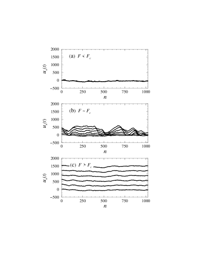
FIG. 15.: Temporal evolution of the displacement profile for the random chain of $N=1024$ beads at different driving forces $F$. The lines plotted are displacement profiles at $t=0,1000,\ldots,5000$, with time step of $\Delta t=0.01$.

We now characterize the roughness of the displacement profile quantitatively close to the critical point. We monitor the disorder-averaged equal-time correlation function,

$$C(n,N)=\frac{1}{N}\sum_{m}\overline{\big{[}\big{(}r_{m+n}(t)-r_{m}(t)-n\;a\big{)}^{2}\big{]}}.$$ (45)

Systems with $N=8$ to $256$ beads were examined right at the threshold forces $F_{c}$. Simulations were run until the systems become “barely pinned”, defined operationally as the point where $v<10^{-3}$. Disorder averages were performed over $5000$ samples for the smaller $N$’s and $100$ samples for the largest $N$.

Numerical results for $C(n,N)$ are shown in Fig. 16 for the random chain. Because of the SOS-like restriction we imposed on the local dynamics, $C^{1/2}(n,N)$ can at most be linear in $n$ as discussed in Ref. [28]. This upper bound is reached by all the curves shown in the figure. Thus $C^{1/2}(n,N)\sim n^{\chi}$, with $\chi\approx 1$. However, the data obviously contain additional dependence on the system size $N$ and suggest the form $C^{1/2}(n,N)=n\cdot N^{\chi_{{\rm FS}}}$, where $\chi_{{\rm FS}}$ is the finite-size exponent. To obtain this exponent,

FIG. 16.: Correlation functions for random spring chains of size $N$. The straight line shows $C(n,N)\sim|n|^{1}$. Inset shows the effective finite-size roughness exponent $\chi_{\rm FS}(N)$, defined by Eq. (46). Dotted line is the suggested asymptotic value of the exponent.

FIG. 17.: Correlation functions for the uniform chains, plotted in the same way as Fig. 16.

we compute an effective exponent $\chi_{FS}(N)$ defined as [28]

$$\chi_{{\rm FS}}(N=2^{i})=\frac{1}{i-1}\sum_{j=2}^{i}\log_{2}\left(\frac{C^{1/2}(2^{j},N)}{C^{1/2}(2^{j-1},N/2)}\right).$$ (46)

The result is shown in the inset of Fig. 16. We see $\chi_{{\rm FS}}(N)$ stabilize for $N>100$, yielding $\chi_{{\rm FS}}=1.22\pm 0.01$ for the random chain. The same calculations finds $\chi_{{\rm FS}}=1.46\pm 0.01$ for the uniform spring chain (Fig. 17).

The obtained value for $\chi_{{\rm FS}}$ in the case of uniform chain is in good agreement with the FRG result [5] which found $\chi_{{\rm FS}}=(4-D+\eta_{s})/2$, with $\eta_{s}=0$ to one-loop order. It is also consistent with the numerical result of $\chi_{{\rm FS}}=1.3\pm 0.3$ found in Ref. [24]. The result for the random chain is also very close to the one reported in Ref. [28] for the simulation of a driven elastic string with random-field or random-bond disorder ($\chi_{{\rm FS}}\simeq 1.25$), and to the ones obtained from the simulations of related models of interface depinning ($\chi_{{\rm FS}}=1.23\pm 0.02$ in Ref. [96], and $\chi_{{\rm FS}}=1.2\pm 0.1$ in Ref. [97]). Combining the results on the two independent exponents $\beta$ and $\chi$, we find strong evidence supporting our expectation that the critical depinning dynamics of the driven random chain is in the same universality class as the driven elastic string in $(1+1)$-dimensional random medium. This is the $D=1$ case of our more general conjecture concerning the critical dynamics of the $D$-dimensional randomly-tethered elastic network. Numerical studies of the dynamics of the two-dimensional system is already underway [75].

V Bulk-mediated Elasticity

So far we have studied the properties of the randomly-tethered elastic network which is completely in contact with a disordered substrate. In many situations however, the elastic medium interacts with the substrate only at one of its surfaces. This is for example the case of friction between a thick piece of rubber and a piece of sandpaper. Similar models have been used to describe aspects of “tectonic plate” movement along an earthquake fault zone (See Fig. 18). Here we extend the model of Sec. IV to include bulk-mediated nonlocal elasticity, and study the driven dynamics of such systems.

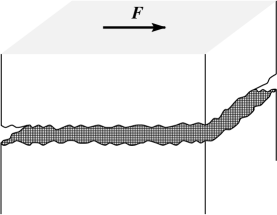
FIG. 18.: Picture illustrating two “tectonic plates” sliding past each other along a “fault zone”.

We shall focus on the $(1+1)$-dimensional caricature of the problem depicted in Fig. 19. We consider a two-dimensional random bead-spring network (of size $L_{x}\times L_{z}$) in contact with a one-dimensional disordered (and impenetrable) substrate $V(x)$ located at $z=0$ (see Fig. 19). We wish to study the dynamics generated by a driving force applied to the upper ($z=L_{z}$) surface. For simplicity, we assume there is a sufficiently large loading force $-F_{N}\hat{z}$ which keeps the elastic network in contact with the substrate, thereby allowing us to suppress the $z$-degrees of freedom in the displacement vectors ${\bf u}$.

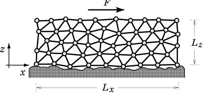
FIG. 19.: A 2D bead-spring system of thickness $L_{z}$ on disordered one-dimensional substrate.

Let the $x$-component of ${\bf u}({\bf R}_{n})$ at the upper and lower boundaries of the array be $w_{0}(n)$ and $w_{1}(n)$ respectively. Consider first the homogeneous elastic medium. The equations of motion for the $w$’s are then

$$\mu^{-1}_{0}\partial_{t}w_{0} = \sum_{n^{\prime}}\left\{-G^{-1}(n-n^{\prime},0)w_{0}(n^{\prime},t)\right.$$ (49)

$$\quad\quad\left.-G^{-1}(n-n^{\prime},L_{z})w_{1}(n^{\prime},t)\right\}$$

$$\quad-V^{\prime}(n\cdot a+w_{0}(n,t))$$

$$\mu^{-1}_{1}\partial_{t}w_{1} = \sum_{n^{\prime}}\left\{-G^{-1}(n-n^{\prime},0)w_{1}(n^{\prime},t)\right.$$ (51)

$$\quad\quad\left.-G^{-1}(n-n^{\prime},L_{z})w_{0}(n^{\prime},t)\right\}+F$$

where $\mu_{i}$’s are the microscopic frictional coefficients, and the $G(n,z)$’s are the Green’s functions whose Fourier transforms are given in Appendix B. We assume that the upper surface $w_{1}$ relaxes very quickly such that the nontrivial dynamics is dominated by the behavior of the lower surface $w_{0}$, due to its contact with the substrate. Setting $\partial_{t}w_{1}=0$ and solving Eq. (51), we obtain a closed equation of motion for $w_{0}$:

$$\mu_{0}\partial_{t}w_{0} = \sum_{n^{\prime}}J(n-n^{\prime})w_{0}(n^{\prime},t)$$ (53)

$$\quad-V^{\prime}(n\cdot a+w_{0}(n,t))+F,$$

where the kernel $J(n)$ is given in term of its Fourier transform

$$\widehat{J}(k) = -2\gamma L_{z}\,\left/\sum_{n=-\infty}^{\infty}\frac{1}{k^{2}+p_{n}^{2}}\right.\,,\quad p_{n}=n\pi{L_{z}}$$ (54)

$$\approx \left\{\begin{tabular}[]{ll}$-2\gamma\left|k\right|$&${\rm for}\quad\left|k\right|L_{z}\gg 1$\\ $-2\gamma L_{z}k^{2}$&${\rm for}\quad\left|k\right|L_{z}\ll 1$\end{tabular}\right.,$$ (57)

as detailed in the Appendix B. Thus, the familiar form of bulk-mediated elasticity, $\widehat{J}(k)\sim-|k|$ is recovered in the limit of large $L_{z},$ while for small $L_{z}$, the problem is effectively one-dimensional in the limit of small $k$.

Randomness in the elastic medium can be readily incorporated into the dynamics. Since the ground state configuration of the beads are unfrustrated, the effect of random spring lengths can be shifted away completely upon using the displacement field $u({\bf R}_{n})$ defined with respect to the equilibrium position ${\bf R}_{n}=(x_{n},z_{n})$ of the beads in the random system (without the external potential $V(x)$). Using $w_{0}(n)=u_{0}(n)+x_{n}-n\cdot a$ in Eq. (53), where $u_{0}(n)=u(x_{n},z_{n}=0)$, we obtain finally the full equation of motion

$$\mu_{0}^{-1}\partial_{t}u_{0} = \sum_{n^{\prime}}J(n-n^{\prime})u_{0}(n^{\prime},t)$$ (59)

$$\quad-V^{\prime}(x_{n}+u_{0}(n,t))+F.$$

The coarse-grained dynamics generated by the discrete system (59) with the kernel (54) can be derived as before. The resultant equation of motion is

$$\mu^{-1}_{0}\,\partial_{t}u_{0}(x,t) = \int_{x^{\prime}}\,J(x-x^{\prime})u_{0}(x^{\prime},t)$$ (61)

$$\quad-V^{\prime}(x)+f_{\rm pin}(x,u_{0})+F,$$

where the pinning force is $f_{\rm pin}(x,u_{0})=V_{>}^{\prime}(x)\delta\rho_{0}(x-u_{0},z=0)$, with $\delta\rho_{0}(x,z)$ being density variation of the relaxed bead-spring system as described before, yielding

$$\overline{[f_{\rm pin}(x,u_{0})f_{\rm pin}(0,0)]}\approx\Delta\delta(x)\delta(u_{0}),$$ (62)

for a variety of randomly-tethered networks.

Eq. (61) with the disorder correlator (62) is very similar to the equation of motion of a contact line which controls the spreading of a non-wetting liquid on a disordered solid surface [98]. As shown by Joanny and de Gennes [99], a contact line is governed by nonlocal elasticity of the form (57), reflecting the energetics of distorting the underlying liquid/gas interface. The driven dynamics of the contact line has been investigated by Ertas and Kardar [100] using the FRG method. A depinning transition similar to that of the driven RM was found. Upon generalizing the substrate to $D$-dimensions, an expansion about the upper critical dimension $D=2$ yields the exponent values $\chi=\epsilon/3$ and $z=1-2\epsilon/9$ to first order in $\epsilon=2-D$. Other exponents can be obtained from the exponent relations $\nu=1/(1-\chi)$, $\beta=(z-\chi)/(1-\chi)$, and $\kappa=D-1+\chi$. Thus the contact line problem ($\epsilon=1$) is described by the exponents $\nu\approx 3/2$, $\beta\approx 7/9$, and $\chi\approx 1/3$. Our problem of course differs from that of the contact line again by the long-range correlations in higher moments of the pinning force $f(x,u_{0})$. However, as in the case of the random spring with local elasticity, we do not expect these higher moments to change the universality class of the depinning dynamics.

To test this conjecture, we performed numerical integration of the discrete equation of motion (59), with the effective kernel $\widehat{J}$ precomputed using (54), with $L_{x}=128$ and $L_{z}=4096$. (Similar results were obtained when we directly used the kernel $\widehat{J}=-2\gamma|k|$.) The parameters describing the springs and the random potential $V$ were the same as the ones used in Sec. IV.B. The data for the velocity-force characteristic (shown in Fig. 20) were obtained by averaging over $15$ independent samples, while the spatial correlation function of $u_{0}(n)$ at $F=F_{c}$ (Fig. 21) was averaged over $100$ samples. From the numerical data, we find the exponents $\beta\approx 0.66$ and $\chi\approx 0.25$, which are consistent with the approximate FRG results for the contact line. Thus the correspondence between the critical dynamics of the random spring chain and that of the directed path appears to hold even with nonlocal elasticity [101].

FIG. 20.: The velocity-force characteristics in the vicinity of the depinning threshold, for the $1+1$ dimensional system of size $128\times 4096$. Log-log plot is shown in the inset. The slope of the straight line gives $\beta=0.66$.

FIG. 21.: Roughness of the displacement field at the threshold $F_{c}=0.1910$. The full line gives $\chi=0.25$. The statistical uncertainties are smaller than symbol size.

We have so far discussed only the critical dynamics of the elastic medium driven at a constant force. Another way the system may be driven is by a constant velocity imposed at the upper boundary. Such situations are of interest to the study of earthquakes [43], as they model tectonic plate motion along a fault. The well-known Burridge-Knopoff model [36] is of this class.

To consider the effect of a constant-$v$ drive, we return first to the linear bead-spring chain described in Sec. IV.B. We drive the chain by connecting each bead $n$ to a reference point $R_{n}^{\ast}$ via a weak loading spring of spring constant $\alpha$. The spacing of the reference points are chosen such that when the beads are in the relaxed state (i.e., without the external potential $V$), the loading springs are unstretched. Thus, $R_{n}^{\ast}=R_{n}=\sum_{m=1}^{n}a_{m}$ where $a_{m}$’s are the lengths of the springs connecting the beads. The reference points are then set to motion, with $R_{n}^{\ast}(t)=R_{n}+vt$. This motion forces the bead-spring chain to move, at the same velocity $v$, via the action of the loading springs (see Fig. 22.)

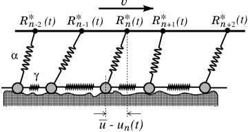
FIG. 22.: A one-dimensional random spring chain pulled by a constant velocity drive via a set of loading springs of spring constant $\alpha$. The mean lag distance is $\bar{u}$.

The equation of motion for the beads is

$$\partial_{t}r_{n} = \gamma[r_{n+1}-2r_{n}+r_{n-1}-(a_{n+1}-a_{n})]$$

$$-\alpha[r_{n}-R_{n}^{\ast}(t)]-V^{\prime}(r_{n}),$$

where $r_{n}(t)$ is the position of the bead $n$. In term of the displacement field $u_{n}(t)=r_{n}(t)-R_{n}^{\ast}(t)+\bar{u}$, ($\bar{u}$ is the mean lag distance as shown in Fig. 22), the equation of motion becomes

$$\partial_{t}u_{n} = \gamma\left[u_{n+1}-2u_{n}+u_{n-1}\right]-\alpha u_{n}$$ (64)

$$\quad-v+\alpha\bar{u}-V^{\prime}(R_{n}+vt+u_{n}(t)-\bar{u}).$$

It is instructive to compare Eq. (64) with Eq. (42) evaluated in the moving frame $r_{n}(t)=R_{n}+vt+u_{n}(t)$:

$$\partial_{t}u_{n} = \gamma\left[u_{n+1}-2u_{n}+u_{n-1}\right]$$ (66)

$$\quad-v-V^{\prime}(R_{n}+vt+u_{n}(t))+F.$$

We find the systems described by (64) and (66) to be statistically the same, up to the damping term $-\alpha u_{n}$, if we identify $\alpha\bar{u}$ in (64) with the driving force $F$. (The random forces $V^{\prime}(x)$ and $V^{\prime}(x-\bar{u})$ clearly have the same statistics.) The knowledge that Eq. (66) exhibits a depinning transition with $v\propto(F-F_{c})^{\beta}$ and a diverging correlation length $\xi\sim(F-F_{c})^{-\nu}$ immediately lead us to conclude that large fluctuations also occur in the system with constant-$v$ drive as $v\rightarrow 0$, with $\xi\sim v^{-\nu/\beta}$ and $\bar{u}\to F_{c}/\alpha$. However, true critical behavior is prevented by the linear damping term $-\alpha u_{n}$ in (64). The correlation length saturates at $\xi^{*}\sim\left(\gamma/\alpha\right)^{1/2}$.

We now turn to the system depicted in Fig. 19, with the upper ($z=L_{z}$) boundary set to constant velocity. Mathematically, the situation is described by Eq. (49), with $w_{1}(n,t)=vt$. The explicit form of the dynamics is readily obtained from the knowledge of $G^{-1}$ (see Appendix B); we find the following equation of motion,

$$\partial_{t}u_{0}(n,t) = \sum_{n^{\prime}}J(n-n^{\prime})\,u_{0}(n^{\prime},t)$$ (68)

$$\quad-\alpha_{L}(u_{0}-vt)-V^{\prime}(x_{n}+u_{0}(n,t))$$

where the kernel $J(n)$ is approximately the same as that describing the constant-$f$ dynamics in Eq. (59), and the damping coefficient is $\alpha_{L}\approx\gamma/(\pi L_{z})$. In the moving frame $u_{0}\rightarrow u_{0}+vt-\bar{u}$, Eq. (68) has the same form as (64) except for the nonlocal elasticity coupling $J$. Thus, we expect similar “near-critical” behavior for the system (68) as $v\rightarrow 0$, with a diverging correlation length $\xi\sim v^{-\nu/\beta}$ which saturates at $\xi^{*}\approx(\gamma/\alpha_{L})^{1/\sigma}$. The value of the exponent $\sigma$ depends on which regime of $J$ the system is in at the scale $\xi^{*}$; see Eq. (57). We have $\sigma=2$ if $L_{z}/\xi^{*}\ll 1$ and $\sigma=1$ if $L_{z}/\xi^{*}\gg 1$. Given the expression for $\alpha_{L}(L_{z})$, we find $\sigma=1$. Thus, $\xi^{*}\sim L_{z}$ becomes very large and the system is very nearly critical as $v\rightarrow 0$. (Note that the lag distance $\bar{u}$ also becomes very large.) Zero-temperature driven dynamics with $v\to 0$ studied here is an example of “extremal dynamics” studied extensively in the context of self-organized critical phenomena [57]. The relation between self-organized criticality and dynamic critical phenomena has been discussed in various contexts [45, 46, 49, 52, 53]. Within our model spring-bead system, we see that the equivalence between these two classes of phenomena can be explicitly established.

We finish this section with a discussion of the ($D+1$)-dimensional generalization of the system depicted in Fig. 19. Our analysis lead us to anticipate strongly that such a system is equivalent to the $D$-component, $D$-dimensional driven manifold in $(D+D)$-dimensional random media, with a nonlocal elasticity kernel (57). In particular, the $D=2$ case is analogous to the sliding slabs of elastic media (Fig. 18). Since $D=2$ is the critical dimension for problems with bulk-mediated elasticity, the critical exponents at the depinning transition are known exactly [2], e.g., $\chi=O(\log)$, $\nu=1$, and $\beta=1$. From these and the exponent relations given above, one finds the exponent describing the avalanches at the onset of motion to be $\kappa=1$. Recently, the avalanche distribution of a related earthquake model was investigated [52]. In the study of earthquakes, one monitors the distribution of the “moment” $M\equiv\int d^{D}{\bf x\,}\Delta u({\bf x})$, where $\Delta u({\bf x})$ is the total displacement at location ${\bf x}$ during an avalanche. Since $\chi=0$ in $D=2$, $M\sim\ell^{2}$ where $\ell$ is the linear size of the avalanche, assuming that the avalanche clusters are compact up to logarithmic correction. From (29), it follows [102] that the probability $\Pr(M)$ of finding an earthquake with moment exceeding $M$ is $\Pr(M)\sim M^{-B}\widehat{\rho}(M/\xi^{2})$ at the critical point, with $B=\kappa/2=1/2$. The model of Ref. [52] uses constant-$v$ drive with $v\rightarrow 0$. Thus, $\xi=\xi^{*}\sim L_{z}$. The numerical result on the moment-distribution is consistent with the RM analogy, as has been pointed out in Ref. [52].

VI Summary

We have presented a detailed study of the static and dynamic properties of an elastic medium interacting with a disordered substrate. The behavior depends crucially on the equilibrium density distribution of the elastic medium in the relaxed state. The interaction of a perfectly homogeneous medium with the substrate belongs to the CDW universality class as has already been discussed in the literature. The somewhat surprising result of this study is that a slight amount of quenched-in inhomogeneities of the elastic medium, even with only interstitials/vacancies or phonons, is sufficient to change the universality class. Instead of the CDW, a $D$-dimensional inhomogeneous medium on $D$-dimensional disordered substrate belongs to the universality class of a $D$-dimensional homogeneous manifold embedded in an effective $(D+D)$-dimensional random medium. This is a consequence of the fact that quenched-in density variation breaks the translational symmetry of the elastic medium, such that the dense/dilute parts of the medium preferentially stick to the attractive/repulsive parts of the substrate. We verified this numerically for a one-dimensional random bead-spring system: The finite-temperature static behaviors of the random chain are found to be indistinguishable from those of the directed path in $(1+1)$-dimensional random medium. The zero-temperature driven dynamics exhibits a depinning transition, the critical properties of which are also indistinguishable from those of the driven elastic string in $1+1$ dimensional random medium. The equivalence is found to hold also for elastic media with nonlocal (bulk-mediated) elasticity, making our model system and results relevant to tribology problems. Finally, a slow-velocity drive is shown to be equivalent to a constant-force drive close to the depinning transition, demonstrating explicitly that self-organized critical phenomenon obtained from certain extremal dynamics may be viewed as a dynamic critical phenomenon.

Although we formulated the interaction of the elastic medium with the substrate in terms of the energetics of density variations, the underlying physics governing the interaction is much more general. The situation being studied here is really one of pattern matching, i.e., matching of quenched-in fluctuations between two different elastic media. This could occur as well in the form of roughness matching, say, the matching of two rough surfaces in contact, or sequence matching, as in the hybridization of two heterogeneous DNA sequences. By viewing interacting random systems as effective homogeneous systems embedded in higher spatial dimension with external randomness, it is possible to simplify and resolve a large class of interesting problems. These include for example the reptation of heteropolymers in disordered gel matrix [55], where “pattern matching” of the polymer composition with its reptation tube leads to anomalously slow dynamics, and the preferential adsorption of heteropolymers on surfaces coated with specific chemical patterns [103]. We hope that this work will stimulate further progress in understanding the physics of interacting random systems.

A Coarse-Grained Dynamics

In this appendix we derive the coarse grained equation of motion (35) (with the definitions (36) – (38)), starting from the discrete model of the inhomogeneous elastic network driven by a constant force. For simplicity, we shall describe only the case $D=2$, and furthermore exclude all quenched-in topological defects including interstitials and vacancies. Inhomogeneities in the medium are described by small deviation ${\bf w}_{n_{1},n_{2}}$ of the equilibrium positions of the beads from a perfect lattice, ${\cal R}_{n_{1},n_{2}}=n_{1}{\bf a}_{1}+n_{2}{\bf a}_{2}$, where the ${\bf a}_{i}$’s are the lattice vectors. For $|{\bf w}|\ll|{\bf a}|$, we can use ${\bf n}\equiv(n_{1},n_{2})$ to label the beads.

We start with the coarse-grained density field,

$$\widetilde{\rho}({\bf r},t)=\frac{1}{\Lambda^{2}}\int_{\Lambda}d^{2}{\bf r}^{\prime}\,\rho({\bf r}+{\bf r}^{\prime})$$ (A1)

where

$$\rho({\bf r})=\sum_{{\bf n}}\delta\left({\bf r}-{\bf r}_{\bf n}(t)\right)$$ (A2)

is the microscopic density field, ${\bf r}_{\bf n}(t)$ gives the actual position of the bead ${\bf n}$, and $\Lambda$ is the coarse-graining scale, of the order of several $|{\bf a}|$’s. In Sec. II, we showed that in terms of the displacement field ${\bf u}({\bf r})$,

$$\rho({\bf r})\approx\bar{\rho}(1-\mbox{\boldmath$\nabla$}\cdot{\bf u})+\delta\rho_{0}({\bf r}-{\bf u}({\bf r})),$$ (A3)

where $\bar{\rho}=1/|{\bf a}_{1}\times{\bf a}_{2}|$ is the average bead density, and $\delta\rho_{0}({\bf x})$ describes the equilibrium density variations. For the specific 2D model considered here,

$$\delta\rho_{0}({\bf x})\sim\bar{\rho}\sum_{j}\cos[{\bf K}_{j}\cdot({\bf x}+{\bf w}({\bf x}))],$$ (A4)

with ${\bf K}_{j}$ being the reciprocal lattice vectors. Since $\delta\rho_{0}({\bf x})$ fluctuates predominantly at the scale $|{\bf a}|$’s, it does not survive the coarse graining, and we have

$$\widetilde{\rho}\approx\bar{\rho}\,(1-\mbox{\boldmath$\nabla$}\cdot{\bf u})$$ (A5)

to leading order in $(\mbox{\boldmath$\nabla$}\cdot{\bf u})$.

The equation of motion for ${\bf u}$ can now be obtained from the evolution of $\rho$, which is given by the continuity equation,

$$\partial_{t}\widetilde{\rho}({\bf r},t)+\mbox{\boldmath$\nabla$}\cdot\widetilde{{\bf j}}({\bf r},t)=0,$$ (A6)

where $\widetilde{{\bf j}}$ is the coarse grained “current”, given by

$$\widetilde{{\bf j}}({\bf r},t)=\frac{1}{\Lambda^{2}}\int_{\Lambda}d^{2}{\bf r}^{\prime}\,{\bf j}({\bf r}+{\bf r}^{\prime},t),$$ (A7)

and

$${\bf j}({\bf r},t)=\sum_{{\bf n}}\partial_{t}{\bf r}_{{\bf n}}\,\delta\left({\bf r}-{\bf r}_{\bf n}(t)\right).$$ (A8)

This choice of the current automatically satisfies the continuity equation, as can be verified directly by inserting the definitions (A1)–(A2), and (A7)–(A8) into Eq. (A6). Using (A5) for $\widetilde{\rho}$ in Eq. (A6), we easily find the form of the equation of motion for ${\bf u}$:

$$\partial_{t}{\bf u}({\bf r},t)=\widetilde{{\bf j}}({\bf r},t)/\bar{\rho}.$$ (A9)

Thus our task is to obtain the coarse-grained current $\widetilde{{\bf j}}$ starting from the discrete equation of motion,

$$\mu_{0}^{-1}\partial_{t}{\bf r}_{\bf n} = \sum_{{\bf a}}\gamma\big{(}{\bf r}_{{\bf n}+{\bf a}}-{\bf r}_{\bf n}+{\bf w}_{{\bf n}+{\bf a}}-{\bf w}_{\bf n}\big{)}+{\bf f}({\bf r}_{\bf n}),$$ (A10)

where the sum is over the nearest neighbors, and

$${\bf f}({\bf r})=-\mbox{\boldmath$\nabla$}V({\bf r})+{\bf F}$$ (A11)

is the external force.

Consider first the “one-particle” equation of motion, $\mu_{0}^{-1}\partial_{t}{\bf r}_{n}={\bf f}({\bf r}_{n}(t))$. Then from the definition (A7), we have

$${\bf j}({\bf r},t) = \mu_{0}\rho({\bf r},t){\bf f}({\bf r})$$ (A12)

$$= \mu_{0}(1-\mbox{\boldmath$\nabla$}\cdot{\bf u})\,{\bf f}({\bf r})+\mu_{0}{\bf f}_{1}({\bf r},{\bf u}(t)),$$ (A13)

where

$${\bf f}_{1}({\bf r},{\bf u})=\delta\rho_{0}({\bf r}-{\bf u})\cdot{\bf f}({\bf r})/\bar{\rho}.$$ (A14)

Upon coarse graining of Eq. (A13), we find

$$\widetilde{{\bf j}}=\mu_{0}(1-\mbox{\boldmath$\nabla$}\cdot{\bf u})\,\widetilde{{\bf f}}({\bf r})+\mu_{0}\,{\bf f}_{\rm pin}({\bf r},{\bf u}(t)),$$ (A15)

where

$$\widetilde{{\bf f}}({\bf r})\equiv\Lambda^{-2}\int_{\Lambda}d^{2}{\bf r}^{\prime}\,{\bf f}({\bf r}+{\bf r}^{\prime})=-\mbox{\boldmath$\nabla$}V_{<}({\bf r})+{\bf F}$$ (A16)

is the coarse-grained force, $V_{<}({\bf r})$ being the slowly varying part of the substrate potential, and

$${\bf f}_{\rm pin}({\bf r},{\bf u})=-\mbox{\boldmath$\nabla$}V_{>}({\bf r})\,\delta\rho_{0}({\bf r}-{\bf u}),$$ (A17)

$V_{>}({\bf r})$ denoting the Fourier modes close to the reciprocal lattice vector ${\bf K}_{i}$’s.

Inclusion of bead-bead coupling as specified by Eq. (A10) only affect the term $\widetilde{{\bf f}}$. For a statistically isotropic array (i.e., a triangular lattice), we find

$$\widetilde{{\bf f}} = (c_{11}({\bf r})-c_{66}({\bf r}))\mbox{\boldmath$\nabla$}(\mbox{\boldmath$\nabla$}\cdot{\bf u})$$ (A19)

$$\quad+c_{66}({\bf r})\nabla^{2}{\bf u}-\mbox{\boldmath$\nabla$}V_{<}({\bf r})+{\bf F}$$

where the elastic moduli $c_{11},c_{66}\sim\gamma a^{2}$. (The ${\bf r}$-dependences of the $c$’s come from $\mbox{\boldmath$\nabla$}\cdot{\bf w}({\bf r})$ and $\mbox{\boldmath$\nabla$}\times{\bf w}({\bf r})$.) The equation of motion for the displacement field ${\bf u}$ is finally

$$\mu_{0}^{-1}\partial_{t}{\bf u}=(1-\mbox{\boldmath$\nabla$}\cdot{\bf u})\,\widetilde{{\bf f}}+{\bf f}_{\rm pin}({\bf r},{\bf u})$$ (A20)

with $\widetilde{{\bf f}}$ and ${\bf f}_{\rm pin}$ given by Eqs. (A19) and (A17) respectively.

B Bulk-Mediated Elasticity

In this appendix, we derive the nonlocal equation describing the motion of the beads at the $z=0$ boundary of an elastic medium placed in $x-z$ half-plane (see Fig. 19). Our strategy is to obtain first the effective Hamiltonian describing the equilibrium fluctuation of the beads at the $z=0$ boundary, subject to various drive conditions applied to the opposing ($z=L$) boundary. The effective equation of motion is then obtained by applying gradient descent dynamics.

We consider here the homogeneous elastic medium which is described by the Hamiltonian (7). To simplify the description, we assume that a sufficiently large normal force is applied such that displacement in the transverse ($z$) direction is negligible. The Hamiltonian describing the residual displacement fluctuation $w(x,z)$ in the $x$-direction can then be written as

$$\beta{\cal H}_{0}\left[u\right]=\int dx\,dz\,\frac{\gamma}{2}\left(\mbox{\boldmath$\nabla$}w(x,z)\right)^{2}.$$ (B1)

The probability to find a system in the state with displacement $w_{0}(x)$ at the $z=0$ boundary and $w_{1}(x)$ at the $z=L_{z}$ boundary is

$$P\left[w_{0},w_{1}\right] \propto \int{\cal D}w\,\delta\left(w(x,0)-w_{0}(x)\right)$$ (B3)

$$\quad\quad\times\;\delta\left(w(x,L_{z})-w_{1}(x)\right)\,e^{-\beta{\cal H}_{0}\left[w\right]}.$$

Integrating out the $w$-field, we obtain

$$P\{w_{0},w_{1}\}\propto e^{-\beta{\cal H}_{{\rm eff}}}$$ (B4)

where

$$\beta{\cal H}_{{\rm eff}} = \int\frac{dk}{2\pi}\left\{\frac{1}{2}G^{-1}(k,0)\left[\left|\widehat{w}_{0}(k)\right|^{2}+\left|\widehat{w}_{1}(k)\right|^{2}\right]\right.$$ (B6)

$$\qquad\qquad\quad\left.-G^{-1}(k,L_{z})\widehat{w}_{0}(k)\widehat{w}_{1}(-k)\right\},$$

with $\widehat{w}_{i}(k)$ being the Fourier transform of $w_{i}(x)$,

$$G^{-1}(k,0) = \frac{C(k,0)}{C^{2}(k,0)-C^{2}(k,L_{z})}$$ (B7)

$$G^{-1}(k,L_{z}) = \frac{C(k,L_{z})}{C^{2}(k,0)-C^{2}(k,L_{z})}$$ (B8)

and

$$C(k,z) = \frac{1}{2\gamma L_{z}}\sum_{p=-\infty}^{\infty}\frac{\cos(pz)}{k^{2}+p^{2}}\,,\quad p=0,\pm\frac{\pi}{L_{z}},\ldots$$ (B9)

$$\approx \left\{\begin{tabular}[]{ll}$\frac{1}{2\gamma|k|}e^{-|k|z}$&${\rm for}\quad|k|L_{z}\gg 1$\\ $\frac{1}{2\gamma L_{z}k^{2}}\left(1+k^{2}L_{z}^{2}/\pi\right)$&${\rm for}\quad|k|L_{z}\ll 1$\end{tabular}\right.$$ (B12)

The equations of motion for $w_{0}$ and $w_{1}$ are now straightforwardly obtained from gradient descent of $\beta{\cal H}_{{\rm eff}}$. For a constant force drive applied to the $z=L_{z}$ boundary, we have

$$\mu^{-1}_{0}\partial_{t}\widehat{w}_{0}(k,t) = -G^{-1}(k,0)\widehat{w}_{0}(k,t)$$ (B14)

$$\quad-G^{-1}(k,L_{z})\widehat{w}_{1}(k,t)$$

$$\mu^{-1}_{1}\partial_{t}\widehat{w}_{1}(k,t) = -G^{-1}(k,L_{z})\widehat{w}_{0}(k,t)$$ (B16)

$$\quad-G^{-1}(k,0)\widehat{w}_{1}(k,t)+F\,\delta(k)$$

where $\mu_{i}$ are the different microscopic frictional coefficients at the boundaries. Assuming that the upper boundary $w_{1}$ relaxes very quickly such that the nontrivial dynamics is dominated by the lower boundary (due to its contact with the substrate), we can set $\partial_{t}w_{1}=0$ and obtain an effective equation for $u_{0}$ itself. It reads in Fourier space

$$\mu_{0}\partial_{t}\widehat{w}_{0}(k,t)=\widehat{J}(k)\widehat{w}_{0}(k,t)+F\,\delta(k)$$ (B17)

with

$$\widehat{J}(k) = -C^{-1}(k,0)$$ (B18)

$$\approx \left\{\begin{tabular}[]{ll}$-2\gamma\left|k\right|$&${\rm for}\quad\left|k\right|L_{z}\gg 1$\\ $-2\gamma L_{z}k^{2}$&${\rm for}\quad\left|k\right|L_{z}\ll 1$\end{tabular}\right..$$ (B21)

Thus, in the limit of large $L_{z}$, the kernel $\widehat{J}$ takes on the form $\widehat{J}(k)=-2\gamma\left|k\right|$ familiar for bulk-mediated elasticity. And in the opposite limit, the coupling becomes local again as the system reverts back to being one-dimensional.

Equation of motion for constant $v$-drive at the $z=L_{z}$ boundary is obtained simply by setting $\widehat{w}_{1}(k,t)=vt\,\delta(k)$ in Eq. (B14). It reads in Fourier space

$$\partial_{t}\widehat{w}_{0}(k,t) = -G^{-1}(k,0)\widehat{w}_{0}(k,t)$$ (B23)

$$\quad+\;G^{-1}(k,L_{z})v_{0}t\,\delta(k).$$

Using the result (B12) in Eqs. (B7) and (B8), we find

$$G^{-1}(k,0) = \left\{\begin{tabular}[]{ll}$2\gamma\left|k\right|$&${\rm for}\quad\left|k\right|L_{z}\gg 1$\\ $\alpha_{L}+\gamma_{L}L_{z}k^{2}$&${\rm for}\quad\left|k\right|L_{z}\ll 1$\end{tabular}\right.$$ (B26)

$$G^{-1}(0,L_{z}) = \alpha_{L}$$ (B27)

with $\alpha_{L}\approx\gamma/(\pi L_{z})$ and $\gamma_{L}\propto\gamma$. Thus the equation of motion for the constant-$v$ drive is

$$\partial_{t}\widehat{w}_{0}(k,t) \approx -\alpha_{L}\left(\widehat{w}_{0}(k,t)-vt\delta(k)\right)$$ (B29)

$$\quad+\widehat{J}(k)\widehat{w}_{0}(k,t),$$

with $\widehat{J}(k)$ given approximately by Eq. (B21).

REFERENCES

- [1]
- [2] See M. Kardar and D. Ertas, in Scale Invariance, Interfaces, and Non-Equilibrium Dynamics, edited by A. McKane, M. Droz, J. Vannimenus, and D. Wolf (Plenum Press, New York, 1995); and references therein.
- [3] H. Fukuyama and P.A. Lett, Phys. Rev. B 17, 535 (1978); P.A. Lee and T.M. Rice, Phys. Rev. B 19, 3970 (1979).
- [4] D.S. Fisher, Phys. Rev. B 31, 1396 (1985).
- [5] O. Narayan and D.S. Fisher, Phys. Rev. B 46, 11520 (1992).
- [6] G. Blatter, M. V. Feigel’man, V.B. Geshkenbein, A.I. Larkin, and V.M. Vinokur, Rev. Mod. Phys. 66, 1125 (1994).
- [7] J. Toner and D.P. DiVicenzo, Phys. Rev. B 41, 632 (1990).
- [8] Y.-C. Tsai and Y. Shapir, Phys. Rev. Lett. 69, 1773 (1992); Phys. Rev. E 50, 3546 (1994); 50, 4445 (1994).
- [9] R. Bruinsma and G. Aeppli, Phys. Rev. Lett. 52, 1547 (1984); J. Koplik and H. Levine, Phys. Rev. B 32, 280 (1985).
- [10] J.L. Cardy and S. Ostlund, Phys. Rev. B 25, 6899 (1982).
- [11] J. Villain and J.F. Fernandez, Z. Phys. B 54, 139 (1984).
- [12] M. Mezard and G. Parisi, J. Phys. (Paris) I 1, 809 (1991).
- [13] T. Giamarchi and P. Le Doussal, Phys. Rev. B 52, 1242 (1995).
- [14] D.S. Fisher, Phys. Rev. Lett. 56, 1964 (1986).
- [15] S. Korshunov, Phys. Rev. B 48, 3969 (1993).
- [16] M. Kardar, and Y.-C. Zhang, Phys. Rev. Lett. 58, 2087 (1987).
- [17] For a review of the directed path in random media, see J. Krug and H. Spohn, in Solids far from equilibrium: Growth, Morphology and Defects, C. Godreche ed. (Cambridge University Press, 1991); and T. Halpin-Healy, and T.-C. Zhang, Phys. Rep. 254, 215 (1995).
- [18] A.A. Middleton, Phys. Rev. E. 52, R3337 (1995).
- [19] C. Zeng et al, Phys. Rev. Lett. 77, 3204 (1996); H. Rieger and U. Blasum, Phys. Rev. B 55, R7394 (1997).
- [20] T. Nattermann, S. Stepanow, L.-F. Tang, and H. Leschhorn, J. Phys. II (France) 2, 1483 (1992); H. Leschhorn, T. Nattermann, S. Stepanow, L.-F. Tang, Annalen der Physik 6, 1 (1997).
- [21] O. Narayan and D.S. Fisher, Phys. Rev. B 48, 7030 (1993).
- [22] D. Ertaş and M. Kardar, Phys. Rev. B 53, 3520 (1996).
- [23] P. Sibani and P.B. Littlewood, Phys. Rev. Lett. 64, 1305 (1990).
- [24] A.A. Middleton and D.S. Fisher, Phys. Rev. Lett. 66, 92 (1991), and Phys. Rev. B 47, 3530 (1993).
- [25] C.R. Myers and J.P. Sethna, Phys. Rev. B 47, 11171 (1993), ibid. 47, 11194 (1993).
- [26] B. Koiller, H. Ji, and M.O. Robbins, Phys. Rev. B 46, 5258 (1992); C.S. Nolle, B. Koiller, N. Martys, and M.O. Robbins, Phys. Rev. Lett. 71, 2074 (1993).
- [27] M. Dong, M.C. Marchetti, A.A. Middleton, and V. Vinokur, Phys. Rev. Lett. 70, 662 (1993).
- [28] H. Leschhorn and L.-H. Tang, Phys. Rev. Lett. 70, 2973 (1993); H. Leschhorn, Physica A 195, 324 (1993).
- [29] L.A.N. Amaral, A.-L. Barabasi, and H.E. Stanley, Phys. Rev. Lett. 73, 62 (1994).
- [30] D. Cule, Phys. Rev. E 52, 1 (1995).
- [31] M.A. Rubio, C.A. Edwards, A. Dougherty, and J.P. Gollub, Phys. Rev. Lett. 63, 1685 (1989).
- [32] V.K. Horváth, F. Family, and T. Vicsek, Phys. Rev. Lett. 67, 3207 (1991).
- [33] S. He, G.L.M.K.S. Kahanda, and P.-Z. Wong, Phys. Rev. Lett. 69, 3731 (1992).
- [34] S.V. Buldyrev et al, Phys. Rev. A 45, R8313 (1992).
- [35] F. Family, K.C.B. Chan, and J. Amar, in Surface Disordering: Growth, Roughening and Phase Transitions, Les Houches Series, (Nova, New York, 1992).
- [36] R. Burridge and L. Knopoff, Bull. Seismol. Soc. Am. 57, 341 (1967).
- [37] H. Takayasu and M. Matsuzaki, Phys. Lett. A 131, 244 (1988).
- [38] J. Carlson and J.S. Langer, Phys. Rev. Lett. 62, 2632 (1989); Phys. Rev. A 40, 6470 (1989).
- [39] H. Nakanishi, Phys. Rev. A 41, 7086 (1990).
- [40] P.A. Thompson and M.O. Robbins, Science 250, 792 (1990).
- [41] H.J.S. Feder, and J. Feder, Phys. Rev. Lett. 66, 2669 (1991).
- [42] D.P. Vallette, and J.P. Golub, Phys. Rev. E 47, 820 (1993).
- [43] J.M. Carlson, J.S. Langer, and B.E. Shaw, Rev. Mod. Phys. 66, 657 (1994).
- [44] P. Bak and C. Tang, Geophys. Rev. B 94, 15635.
- [45] K. Chen, P. Bak, and S.P. Obukhov, Phys. Rev. A 43, 625 (1991).
- [46] C. Tang and P. Bak, Phys. Rev. Lett. 60, 2347 (1988).
- [47] P. Bak, C. Tang, and K. Wiesenfeld, Phys. Rev. Lett. 59, 381 (1987).
- [48] C. Tang, K. Wiesenfeld, P. Bak, S. Coppersmith, and P. Littlewood, Phys. Rev. Lett. 58, 1161 (1987).
- [49] O. Narayan and A.A. Middleton, Phys. Rev. B 49, 244 (1994).
- [50] P. Miltenberger, D. Sornette and C. Vanette, Phys. Rev. Lett. 71, 3604 (1993); P.A. Cowie, C. Vanette and D. Sornette, J. Geophys. Res. 98, 21809 (1993).
- [51] D. Cule, and T. Hwa, Phys. Rev. Lett. 77, 278 (1996).
- [52] D.S. Fisher, K. Dahmen, S. Ramanathan and Y. Ben-Zion, Phys. Rev. Lett. 78, 4885 (1997).
- [53] M. Paczuski and S. Boettcher, Phys. Rev. Lett. 77, 111 (1996).
- [54] T. Hwa, M.C. Marchetti, and V.M. Vinokur (unpublished).
- [55] D. Cule and T. Hwa, preprint (cond-mat/9706262).
- [56] T. Hwa and M. Lässig, Phys. Rev. Lett. 76, 2591 (1996).
- [57] M. Paczuski, S. Maslov, and P. Bak, Phys. Rev. E 53, 414 (1996).
- [58] L.D. Landau and E.M. Lifshitz, Theory of Elasticity, (Pergamon Press, London, 1959).
- [59] The elastic moduli have space-dependent components due to the presence of quenched randomness in the medium; however short-ranged variations are irrelevant as can be easily checked.
- [60] A random torque coupling to will be generated by the interaction and may be included in Eq. (12) for completeness. However, this and the random compression term are both irrelevant as we will see.
- [61] C. Carraro, and D.R. Nelson, Phys. Rev. E 56, 797 (1997).
- [62] D. Carpentier and P. LeDoussal, Phys. Rev. B 55, 12128 (1997).
- [63] P. Le Doussal and T. Giamarchi, Phys. Rev. Lett. 74, 606 (1995); J. Kierfeld, J. Phys. (France) I 5, 379 (1995).
- [64] G.G. Batrouni and T. Hwa, Phys. Rev. Lett. 72, 4133 (1994); D. Cule and Y. Shapir, Phys. Rev. Lett. 74, 114 (1995) and Phys. Rev. B 51, 3305 (1995); H. Rieger, Phys. Rev. Lett. 74, 4964 (1995); E. Marinari, R. Monasson, J.J. Ruiz-Lorenzo, J. Phys. A 28, 3975 (1995).
- [65] T. Hwa and D.S. Fisher, Phys. Rev. Lett. 72, 2466 (1994).
- [66] T. Halpin-Healy, Phys. Rev. Lett. 62, 442 (1989); Phys. Rev. A 42, 711 (1990).
- [67] For a recent review, see L. Balents, Lecture notes for the Beg-Rohu Spring School on Disordered Systems, available online at http://www.itp.ucsb.edu/ balents/bignotes/bignotes.html.
- [68] For the random manifold, linear terms such as in the Hamiltonian (12) are irrelevant.
- [69] D.R. Nelson and V.M. Vinokur, Phys. Rev. B 48, 13060 (1993).
- [70] T. Hwa, D.R. Nelson, and V.M. Vinokur, Phys. Rev. B 67, 1167 (1993).
- [71] J. Krug and T. Halpin-Healy, J. Phys. I (France) 3, 2179 (1993); I. Arsenin, J. Krug and T. Halpin-Healy, Phys. Rev. E 49, R3561 (1994).
- [72] N. Hatano and D.R. Nelson, Phys. Rev. Lett. 77, 570 (1996).
- [73] In Ref. [56], the irrelevancy of correlated disorder for a closely related sequence alignment problem was conjectured based on similar reasons.
- [74] More generally, if the dimensionality of and are and respectively, then the problem is equivalent to that of a -component random manifold in -dimensions.
- [75] C. Zeng et al, private communication (1997).
- [76] We are grateful to D.R. Nelson for suggestions and discussions. See also Ref. [61] for discussions.
- [77] C. Carraro and D.S. Fisher, Phys. Rev. B 51, 534 (1995).
- [78] We are indebted to D.S. Fisher for an illuminating discussion on the significance of the relabeling symmetry breaking in the context of the one-dimensional random-spring system.
- [79] A similar disorder correlator was obtained in Appendix A of Ref. [13].
- [80] M. Kardar, in Fluctuating Geometries in Statistical Mechanics and Field Theory - Les Houches, Vol. 62, edited by F. David, P. Ginsparg, and J. Zinn-Justin (Elsevier, Amsterdam, 1996).
- [81] E. Medina, T. Hwa, M. Kardar and Y.-C. Zhang, Phys. Rev. A 39 3053, (1987).
- [82] D.S. Fisher and D.A. Huse, Phys. Rev. B 43 10728, (1991).
- [83] J.M. Kim, M.A. Moore, and A.J. Bray, Phys. Rev. A 44, 2345 (1991); J.M. Kim, A.J. Bray, and M.A. Moore, Phys. Rev. A 44, R4782 (1991).
- [84] The avalanche distribution was discussed in the context of CDW in Ref. [49], and extended to RM in Ref. [21] . The exponent relation for relies on argument relating the critical behaviors as and .
- [85] H. Ji and M.0. Robbins, Phys. Rev. B 46, 14519 (1992).
- [86] J. Krug, Phys. Rev. Lett. 75, 1795 (1995).
- [87] L. Balents and M.P.A. Fisher, Phys. Rev. Lett. 75, 4270 (1995).
- [88] Some of the terms have also been obtained in T. Giamarchi and P. Le Doussal, Phys. Rev. Lett. 76, 3408 (1996).
- [89] The term is used in RG calculations [62] as a “bookkeeping” device to keep track of fluctuations in .
- [90] For certain anisotropic driven system [29], the coefficient of the terms does not vanish even as ; see Ref. [91] for a detailed discussion. This is however not the case here.
- [91] L.-H Tang, M. Kardar, and D. Dhar, Phys. Rev. Lett. 74, 920 (1995).
- [92] The kinetic term is again irrelevant right at the depinning transition as in the CDW case.
- [93] The regime of overlapping avalanches was studied in Ref. [94] for the sandpile model. The dynamics in this regime was shown to be described by the driven-diffusion equation, which is a nonlinear Langevin equation. For the problem at hand, the moving phase with overlapping avalanches is described analogously by the KPZ equation [95].
- [94] T. Hwa and M. Kardar, Phys. Rev. A 45, 7002 (1992).
- [95] M. Kardar, G. Parisi, and Y.-C. Zhang, Phys. Rev. Lett. 56, 889 (1986).
- [96] S. Maslov, M. Paczuski, and P. Bak, Phys. Rev. Lett. 73, 2162 (1994).
- [97] S. Roux and A. Hansen, J. de Physique I 4, 515 (1994).
- [98] P.G. de Gennes, Rev. Mod. Phys. 57, 827 (1985).
- [99] J.F. Joanny and P.G. de Gennes, J. Chem. Phys. 81, 552 (1984).
- [100] D. Ertas, and M. Kardar, Phys. Rev. E 49, R2532 (1994).
- [101] To test our results more quantitatively, it would be useful to compare directly with the numerics of the contact line depinning when it becomes available.
- [102] More generally, , where is the fractal dimension of the avalanche cluster, yielding .
- [103] T. Hwa and D. Cule, preprint (cond-mat/9707079).
- [104] K.V. Samokhin, JETP Lett. 64, 580 (1996); ibid. 853 (1996).