[

The Lower Critical Dimension of the $XY$ Spin Glass

Abstract

We investigate the $XY$ spin-glass model in two and three dimensions using the domain-wall renormalization-group method. The results for systems of linear sizes up to $L=12$ (2D) and $L=8$ (3D) strongly suggest that the lower critical dimension for spin-glass ordering may be $d_{\rm c}\approx 3$ rather than four as is commonly believed. Our 3D data favor the scenario of a low but finite spin-glass ordering temperature below the chiral transition but they are also compatible with the system being at or slightly below its lower critical dimension.

]

It has been known since the early work of Villain[1] that frustrated planar models possess, in addition to the continuous degeneracy associated with spin rotations, a discrete two-fold degeneracy associated with the invariance of the Hamiltonian under a reflection about an arbitrary direction. As a consequence, each plaquette has an Ising-like degree of freedom, the chirality, that corresponds to the handedness of the configuration of the spins around it. It is also well established[2, 3, 4, 5] that in two and three dimensions chiral and spin variables decouple at long distances and order separately[6]. In 2D long range chiral and spin order appear simultaneously at zero temperature, but the transition is unusual in that there are two independent divergent correlation lengths as $T\to 0$[2, 3]. While there is convincing evidence[2, 4, 5] that in 3D the chiral-glass transition occurs at a finite temperature $T_{\rm CG}$, existing Monte Carlo simulations[5, 7] and studies of the scaling of defect energies at zero temperature[2, 5] suggest that spin-glass order sets in at $T_{\rm SG}=0$ just as in two dimensions. These, as well as older numerical results[8, 9, 10] have led to the belief that the lower critical dimension (LCD) for spin-glass order in this model is $d_{c}\geq 4$, a conjecture that is widely accepted even if a rigorous proof has turned out to be elusive[11, 12, 13]. The limitations inherent to the numerical methods raise some doubts about the robustness of this conclusion, however. The systems studied with the defect-energy method are rather small. While the domain wall energy flows towards weak coupling with increasing linear size $L$ for systems with $L\leq 4$[10], more recent simulations[5] for $L\leq 6$ show a tendency towards saturation for the bigger sizes. It is thus conceivable that the systems studied up to now are still far from the scaling regime. The Monte Carlo simulations[5, 7] were for much larger lattices but the rapid increase in the thermalization times with decreasing $T$ makes it impossible to attain the relevant temperature region, $T\ll T_{\rm CG}$. It appears that is also difficult to reach the asymptotic regime with this technique. Indeed, Kawamura[5] has noticed that the Binder function associated with the spin-glass order parameter fails to show scaling behavior in the temperature range covered by his simulations, $T\gtrsim T_{\rm CG}$. The spin-glass susceptibility does seem to scale but Jain and Young[7] found that their data can be fitted with comparable accuracy by assuming such different values of the spin-glass critical temperature as $T_{\rm SG}=0$ and $T_{\rm SG}=0.45J$. In view of such uncertainties we may still regard the nature of the low-temperature phase of the 3D $XY$ spin-glass as an open problem.

In this paper we study the $XY$ spin-glass model in two and three dimensions with the domain-wall renormalization-group method (DWRG)[8, 9] . Using a new and powerful algorithm for the search of ground-state energies we have been able to study systems with linear sizes up to $L=12$ (in 2D) and $L=8$ (in 3D). In both cases our largest system contains more than twice as many spins as have been considered before. Our results in 2D agree with those found by other authors[2], confirming that the scaling regime had been reached in previous simulations. This turns out not to be the case in three dimensions, where we find that there is a crossover between small- and large-$L$ behavior at $L\approx 5$. The domain-wall energies scale as $W\sim L^{\lambda}$. The sign of the stiffness exponent $\lambda$ may be positive or negative depending on whether the system is above or below its LCD. We find $\lambda_{\rm c}=0.5\pm 0.2$ and $\lambda_{\rm s}=0.056\pm 0.11$ for chiral and spin domain walls, respectively. The fact that $\lambda_{\rm c}>0$ is the signature that there is long-range chiral order at low-temperature in the system as found by other authors[2, 5]. The smallness of $\left|\lambda_{\rm s}\right|$ constitutes to our knowledge the first numerical evidence that the LCD of the $(\pm J)$ $XY$ model may be close to three. Two scenarios are compatible with the measured value of $\lambda_{\rm s}$, i) a spin-glass transition at a finite temperature $T_{\rm SG}\ll T_{\rm CG}$ or ii) a zero-temperature transition with the correlation length $\xi\sim T^{-\nu}$ and $\nu\gg 1$. Statistics favors the former.

The Hamiltonian of the model is

$$H=-\sum_{<ij>}J_{ij}\ \cos\left(\theta_{i}-\theta_{j}\right),$$ (1)

where the sum runs over all pairs of nearest-neighbor sites of the 2D square or 3D cubic lattices. The exchange couplings $J_{ij}$ are random independent variables that take the values $J=+1$ and $J=-1$ with equal probability. In the DWRG method[8, 9] one studies the sensitivity of the system to changes in the boundary conditions at $T=0$. The ground-state energies of an ensemble of systems of size $L^{D}$ are calculated using periodic (P) and anti-periodic (AP) boundary conditions along a given direction while keeping fixed boundary conditions along the $(d-1)$ remaining directions. The width of the distribution of differences of ground-states energies, $W_{\rm s}(L)=[\left(E_{\rm P}-E_{\rm A}\right)^{2}]^{1/2}_{J}$ is interpreted as an effective coupling constant between blocks of $L^{D}$ spins. This is expected to scale as $W(L)\sim L^{\lambda}$ for large enough $L$. If the stiffness exponent, $\lambda$, is positive the rigidity of a block diverges with its size, a sign that there is long-range order in the system. If $\lambda<0$ there exists a length scale $L^{-|\lambda|}\sim T$ beyond which the effective coupling between blocks becomes smaller than the temperature. This scale is identified with the correlation length and the correlation-length exponent is obtained from $\nu=1/|\lambda|$[10]. Chiral ordering may be studied similarly except that the calculation requires knowledge of the ground-state energy for reflective boundary conditions as well as the other two[2].

The success of this approach relies on the availability of an efficient and accurate way of finding the lowest-lying states of the system. In the usual spin-quench algorithm[14] (SQA) one randomly generates long sequences of metastable configurations among which one hopes to find the ground-state or states sufficiently close in energy. The number of metastable states of a frustrated system increases rapidly with its size (probably exponentially[10]) and so does the number of trials that need to be performed to have a non-negligible chance of finding a relevant state. This fact restricts severely the sizes of the systems that can be studied using this method. In order to go beyond the limits of the SQA we have developed a ground-state search algorithm of far greater efficiency. This algorithm is inspired by some of the morphological features of the low-lying states of the frustrated $XY$ model that are as follows[15, 16]. i) In a given sample there are regions with a low density of frustrated plaquettes where the spins form almost collinear domains, and regions where frustration is high and the spin arrangement looks random. The position, size and shape of the domains are mostly determined by the random bond realization and hardly vary from one state to another. ii) Apart from smooth spin-wave-like distortions, the essential differences between the spin configurations of any two low-energy states are large amplitude, almost rigid rotations of the individual domains, and chirality reversals of a fraction of the frustrated plaquettes in the regions separating them. The energies of states that do not have this structure are much higher[16, 15]. Our method suceeds in preserving the domain structure at each stage of the procedure by treating the spins in high local fields (domain spins) differently from those in the more frustrated regions. In this way the appearance of uninteresting high-energy configurations becomes unlikely. The algorithm will be sketched in the following paragraph. Full details will be given in a separate publication[16].

The initial (or parent) state of the sequence, $\{\theta_{\rm 0}\}$, is obtained by a conjugate-gradient minimization (CGM) of the energy with a random spin distribution as initial condition. Next, new spin configurations are generated by iterating the following loop any number of times. i) The spins in the $n$-th configuration $\{\theta_{\rm n}\}$ are divided into two groups according to whether their local field $h_{i}=\sum_{j}J_{ij}\cos\left(\theta_{i}-\theta_{j}\right)$ is greater or smaller than an appropriately chosen threshold field, $0\leq h_{t}\leq 2D$ (see below). The spins in the first group are defined as the domain spins. ii) Existing correlations between the domains and the rest of the system are broken by means of a random rigid rotation of the former. iii) A fraction $p$ of the spins in weak local fields are randomly picked and their orientations are randomly reset. iv) The energy of the subsystem of domain spins is minimized with the rest of the spins held fixed. v) The resulting configuration is let to relax performing a CGM of the total energy of the system. The outcome is the next state in the sequence, $\{\theta_{\rm n+1}\}$. vi) The energy of this state is stored and $h_{t}$ is rescaled if necessary (see below). vii) End of the loop.

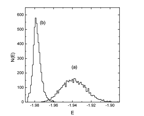
FIG. 1.: Distribution of the energy per spin E of two series of 5 000 metastable states each of one realization of the $XY$ $J=\pm 1$ spin glass on a 512-site 3D lattice. The states have been generated using the spin-quench method (a) and the algorithm described in the text (b).

The parameter $h_{t}$ must be carefully chosen for this algorithm to be efficient. It defines the degree of collinearity required of an ensemble of spins for it to qualify as a domain ($h_{t}=2D$ for perfectly aligned spins in an homogeneous environment). If $h_{t}$ is set very high, too many spins are involved in step iii) above and the domain structure is not preserved. In this regime the method is equivalent to the SQA where all the spins are randomly reset at each step. On the other hand, too small a threshold field leads to trapping, i.e., all the states of the sequence are in the vicinity of the parent state. There is an optimum value of the threshold field in between these extreme cases. In the running version of our code the performance of the algorithm is continuously monitored and a procedure has been devised that allows $h_{t}$ to self-adjust when degradation is detected. This method is particularly appropriate for the treatment of large systems. This is illustrated in Fig. 1 which shows the energy distributions of two sequences of metastable states of the same realization of a disordered 3D system of $N=8^{3}$ spins with anti-periodic boundary conditions. Histograms (a) and (b) have been obtained from 5000 energy levels each generated using the SQA and our algorithm, respectively. In the latter case we have verified that trapping had not occurred by making sure that the same histogram results from sequences originating from different parent states. Distributions (a) and (b) are quite different. Whereas the histogram of the energy levels obtained with the standard method is wide and peaks at high energies, that of our sequences is much narrower and is concentrated in the low-energy end of the spectrum. It is remarkable that most of the energies found with the new method lie in a region where the SQA did not find any state after the same number of trials. The calculation with our method takes only 20% more CPU time than that with the traditional one.

We have used this method to perform DWRG calculations for two- and three-dimensional systems. Much is known about the two-dimensional case which therefore serves as a test of our methods. We have determined spin and chiral defect energies for systems of size $L\times L$ with $L$=4,5,6,7,8,10 and 12. The disorder averages were taken over 128000 ($L$=4), 64000 ($L$=5), 12800 ($L$=6 and 7), 6400 ($L$=8), 2560 ($L$=10) and 1280 ($L$=12) independent bond configurations, respectively. The ground state energy was estimated from the analysis of sequences containing 20 ($L$=4), 50 ($L$=5), 100 ($L$=6), 200 ($L$=7 and 8), 1500 ($L$=10), and 3000 ($L$=12) states. Low-energy states were accepted as ground-state candidates only if they and their chirality-reversed partners appeared several times in the sequence at widely spaced positions. This guarantees that the states in the sequence come from well separated regions of phase-space. A log-log plot of the size dependence of the two-dimensional defect energies is shown in Fig. 2. The symbols are the numerical results and the dashed lines are fits to a power-law. The fits are of good quality even for small $L$. The renormalized stiffness decreases with increasing $L$ for both types of domain wall indicating that spin and chiral variables only order at zero temperature. From the slopes determined by the fits we can compute the correlation length exponents for the two transitions. We find $\nu_{\rm s}=1.29\pm 0.02$ and $\nu_{\rm c}=2.57\pm 0.003$ for the spin and chiral order parameters, respectively. These values are in good agreement with the results of Kawamura and Tanemura[2] who find $\nu_{\rm s}=1.2\pm 0.15$ and $\nu_{\rm c}=2.6\pm 0.3$, respectively in their DWRG calculations for systems with $L\leq 8$. Moreover, the value of the chiral exponent deduced from our data is very close to the correlation length exponent of the 2D Ising spin-glass obtained by Monte Carlo[17] ($2.6\pm 0.4$) or transfer-matrix[18] ($2.59\pm 0.13$) methods. This agrees with the view that the chiral transition in the $XY$ spin glass model is in the Ising universality class.

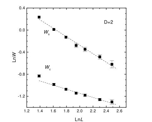
FIG. 2.: The $L$-dependence of the spin (squares) and chiral (circles) domain-wall energies of the $(\pm J)$ $XY$ spin-glass model on $L\times L$ square lattices. Where not drawn the statistical error bars are smaller than the size of the data points. The dashed lines are the power-law fits mentioned in the text.

We now turn to the results for three-dimensional systems. Much longer sequences of stationary states are needed to determine the ground-state energy in this case. Our series consist of 100 ($L$=3), 200 ($L$=4), 500 ($L$=5), 1000 ($L$=6), 3000 ($L$=7) and 5000 ($L$=8) states, respectively. Moreover, the results for the bigger lattices were further checked by repeating the calculation starting form three different parent states. Sample averages were taken over 25600 ($L$=3), 6400 ($L$=4), 1280 ($L$=5,6), 640 ($L$=7) and 128 ($L$=8) samples, respectively. The $L$-dependence of the effective couplings in three dimensions is shown by the symbols in Fig.  3. An important difference with the 2D case is that a crossover region is clearly seen around $L$=5. Power-law behavior, shown in the figure by the dashed lines, is only observed for the largest lattices. We first discuss the chiral degrees of freedom. As found in previous studies[2, 5], $W_{\rm c}$ flows towards strong coupling signaling the existence of finite-temperature chiral-glass transition in the infinite system. From the fits shown in the figure we can estimate the chiral stiffness exponent $\lambda_{\rm c}=0.56\pm 0.18$.

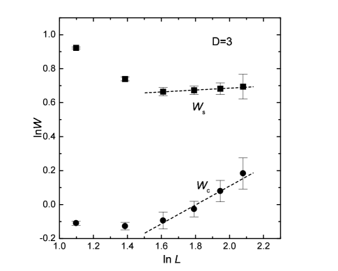
FIG. 3.: The $L$-dependence of the spin (squares) and chiral (circles) domain-wall energies for the $(\pm J)$ $XY$ spin-glass model on $L\times L\times L$ simple cubic lattices. The dashed lines are the power-law fits mentioned in the text.

The spin domain-wall-energy decreases rapidly with $L$ for small sizes but it exhibits a much slower variation for $L\gtrsim 5$. This behavior was not observed in older simulations[2] but Kawamura’s more recent DWRG results distinctively show the beginning of the saturation of the spin defect energy for $L\sim 5$. Fitting the results for the four largest sizes with a power-law we find the spin-stiffnes exponent $\lambda_{\rm s}=0.056\pm 0.11$. The large error bar is due to poor statistics in the case of our largest size for which the sample average could only be taken over 128 configurations of the bonds. The error in the determination of the ground-state energy, estimated from a comparison of the results of searches conducted starting from different parent states, is much lower. It is worth mentioning that if we make the fit omitting the last point the result is $\lambda_{\rm s}=0.052\pm 0.03$.

The smallness of $|\lambda|$ suggests that the LCD of the $(\pm J)$ $XY$ model is close to three. The data statistically favor $\lambda_{\rm s}\gtrsim 0$. If this is the case the spin-glass transition temperature should be finite with $T_{\rm SG}\ll T_{\rm CG}$ as implied by our finding that $\lambda_{\rm c}\gg|\lambda_{\rm s}|$. The numerical results are also compatible with a second and far less exciting possibility, a zero-temperature transition with an unusually large correlation-length exponent.

There exist no theoretical objections against a spin-glass transition below $T_{\rm CG}$ since the proofs[11, 13] of the absence of SG ordering in the three-dimensional model at finite $T$ fail if reflection-symmetry is broken[5, 12, 13] as is the case when chiral-glass order is present. The possibility of a finite-temperature SG transition discussed here is thus restricted to the case of the $XY$ model for which one can convincingly argue that $T_{\rm CG}\neq 0$. The case of the Heisenberg model seems quite different in that the role of the chiral variables is not as clear as in the planar model and there is no evidence of the existence of chiral order at finite temperatures. Therefore we still expect isotropic three-dimensional spin-glass models to have an ordered phase only at zero temperature[8, 9, 19].

We thank Professors H. Nishimori and H. Kawamura for helpful correspondence and T. Ziman for a critical reading of the manuscript. The calculations reported in this work have been performed on the 256-processor CRAY T3E parallel computer at the ‘Centre Grenoblois de Calcul Vectoriel’. We thank the staff for technical help.

REFERENCES

- [1] J. Villain, J.Phys. C 10, 4793 (1977) and J.Phys. C 11, 745 (1978).
- [2] H. Kawamura and M. Tanemura, J. Phys. Soc. Jpn. 60, 608 (1991).
- [3] P. Ray and M. A. Moore, Phys. Rev B 45, 5361 (1992).
- [4] H. Kawamura, J. Phys. Soc. Jpn. 61, 3062 (1992).
- [5] H. Kawamura, Phys. Rev B 51, 12 398 (1995).
- [6] In a recent preprint (cond-mat/9703162 ) S. Jain has suggested that this may not be true in four dimensions.
- [7] S. Jain and A. P. Young, J. Phys. C 19, 3913 (1986).
- [8] J. R. Banavar and M. Cieplak, Phys. Rev. Lett. 48, 832 (1982); M. Cieplak and J. R. Banavar, Phys. Rev. B 29, 469 (1984).
- [9] W. L. McMillan, Phys. Rev. B 31, 342 (1985).
- [10] B. M. Morris, S. G. Colborne, M. A. Moore, A. J. Bray and J. Canisius, J. Phys. C 19, 1157 (1986).
- [11] H. Nishimori and Y. Ozeki, J. Phys. Soc. Jpn. 59, 289 (1990).
- [12] M. Schwartz and A. P. Young, Europhys. Lett. 15, 209 (1991).
- [13] Y. Ozeki and H. Nishimori, Phys. Rev. B 46, 2879 (1992).
- [14] L. R. Walker and R. E. Walstedt, Phys. Rev. B 22, 3816 (1980).
- [15] P. Gawiec and D. R. Grempel, Phys. Rev. B 44, 2613 (1991).
- [16] P. Gawiec, D. R. Grempel and J. Maucourt, to be published.
- [17] R. N. Bhatt and A. P. Young, Phys. Rev. Lett. 54, 245 (1985); Phys. Rev. B 37, 5606 (1988).
- [18] H. F. Cheung and W. L. McMillan, J. Phys. C 16, 7027 (1983).
- [19] F. Matsubara, T. Iyota, and S. Inawashiro, Phys. Rev. Lett. 67, 1458 (1991).