Shear-Induced Isotropic-to-Lamellar Transition in a Lattice-Gas Model of Ternary Amphiphilic Fluids

Abstract

Although shear-induced isotropic-to-lamellar transitions in ternary systems of oil, water and surfactant have been observed experimentally and predicted theoretically by simple models for some time now, their numerical simulation has not been achieved so far. In this work we demonstrate that a recently introduced hydrodynamic lattice-gas model of amphiphilic fluids is well suited for this purpose: the two-dimensional version of this model does indeed exhibit a shear-induced isotropic-to-lamellar phase transition.

PACS numbers: 82.70.-y;05.70.Lm

I Introduction

Soft materials such as polymer solutions, liquid crystals, surfactants, and microemulsions are frequently processed or utilized through the application of large deformations. Various attempts have been made to investigate and characterise the behaviour of such complex systems under conditions such as shear flow, for which there are numerous industrial applications [1]. In this letter we model the effect of linear shear flow on a hydrodynamic, isotropic, sponge microemulsion phase using our recently introduced lattice-gas automaton model for simulating self-assembling amphiphilic systems [2]. Experimental results [3, 4, 5] as well as theoretical predictions [6] provide evidence for the presence of a transition from an isotropic to a lamellar phase in such systems; however, we are unaware of any model that is capable of simulating complex multi-phase flow of this sort. This is because of the considerable difficulty involved in simulating ternary amphiphilic systems under hydrodynamic flow, as well as in the implementation of the boundary conditions required for shear. Traditional continuum based fluid-dynamical modelling methods, such as finite-difference, finite-element or volume-of-fluid techniques cannot viably deal with the complexity involved; molecular dynamics, on the other hand, are too computationally expensive.

Hydrodynamic lattice-gas models have evolved from simulating simple one-component Navier-Stokes fluids [7], to two- and multi-component immiscible fluids [8]. We have recently extended such models to systems including amphiphiles [2]. Lattice-gas models can reproduce fluid dynamics on mesoscopic and higher levels, permitting the investigation of non-equilibrium (kinetic) behaviour over a broad range of length and time scales [9]. The relative simplicity of the collision rules, the self-assembly of complex interfaces, the presence of natural underlying kinetic fluctuations and the ease of implementation of complex boundary conditions suggest that such hydrodynamic lattice-gas models are an appropriate choice for the study of amphiphilic fluids under linear shear.

Linear shear flow has previously been applied to binary fluid systems in both two [10] and three-dimensional [11] lattice-gas models. We make use of the method introduced in the second of these papers for obtaining linear shear flow on the lattice, although some modification is required for our ternary amphiphilic system.

As well as simulating the shear-induced isotropic-to-lamellar transition, this work was undertaken in order to investigate further the validity of our amphiphilic model for complex fluid simulation. This is the first application of the model to the simulation of known physical effects associated with bulk fluid flow. In Section II we briefly describe our model and the numerical techniques we have used to investigate the system under shear; our simulations are presented in Section III with concluding remarks in Section IV.

II Model and Analysis

We perform simulations using our hydrodynamic lattice-gas model of amphiphilic systems as previously published [2]. The model is a microscopic dynamical system which gives the correct mesoscopic and macroscopic behaviour of mixtures of oil, water and surfactant. The model is based on the two-fluid immiscible lattice-gas of Rothman and Keller [12], which we have reformulated using a microscopic particulate description to permit the inclusion of amphiphile. Pursuing the electrostatic analogy with the Rothman-Keller model, we describe surfactant molecules as dipoles, characterised by a dipole vector $\sigma$. The model exhibits the commonly formed equilibrium microemulsion phases, including droplets, sponge structures (the two-dimensional analogue of the bicontinua in three dimensions) and lamellae [2]. Moreover, the lattice-gas model conserves momentum as well as the masses of the various species, and correctly simulates fluid dynamical and scaling behaviour during self-assembly of these phases [13, 14].

It should be noted that, formally, no lamellar phase can exist at finite temperature in two spatial dimensions: thermal fluctuations are large enough to destroy true long-range smectic order. We showed in our original paper that the stability of such relatively small and artificially created structures is greatly enhanced compared to that observed in the absence of surfactant or when amphiphilic interactions are extinguished in a ternary fluid [2]. A more thorough investigation of the relative stability of the observed lamellae remains as work for the future.

In order to incorporate the most general form of interaction energy within our model system, we introduce a set of coupling constants $\lambda,\mu,\epsilon,\zeta$, in terms of which the total interaction energy can be written as [2]

$$\Delta H_{\mbox{int}}=\lambda\Delta H_{\mbox{cc}}+\mu\Delta H_{\mbox{cd}}+\epsilon\Delta H_{\mbox{dc}}+\zeta\Delta H_{\mbox{dd}}.$$ (1)

The four terms on the right hand side correspond, respectively, to the relative immiscibility of oil and water, the tendency of surfactant to surround oil or water droplets, the propensity of surfactant dipoles to align across oil-water interfaces and the contribution from pairwise interactions between surfactant molecules. For consistency we choose these coefficients to be of the same value for all simulations in this paper, which allow a sponge microemulsion phase to form in one part of the ternary phase diagram [2]; as such these are,

$$\lambda=1.0,\mu=0.05,\epsilon=8.0,\zeta=0.5.$$ (2)

As stated above, in order to investigate the effect of linear shear flow on a sponge microemulsion phase we apply a technique devised by Olson and Rothman [11] for shearing two-component binary lattice-gas fluids, which we have adapted to meet the requirements of our amphiphilic lattice-gas model. The technique provides a linearly varying, tunable velocity gradient in a direction orthogonal to the flow (see Fig. 1). The velocities used are small enough to ensure that the lattice gas accurately represents the hydrodynamic flow [11].

We analyse the simulation results in three ways. The first is direct visualisation of the growth of domains both with and without the imposition of a shear velocity. The second, performed in order to observe any anisotropic domain growth and the formation of a characteristic Bragg peak in the presence of shear, is a quantitative analysis of the structure factor for the oil-water density difference,

$$S({\bf k},t)=\frac{1}{N}\left|\sum_{{\bf x}}(q({\bf x},t)-q^{av})e^{i{\bf k}\cdot{\bf x}}\right|^{2},$$ (3)

where ${\bf k}=\left(2\pi/L\right)\left(m{\bf i}+n{\bf j}\right)$, $m,n=1,2,...,\frac{L}{2}$, q(x,t) is the water-minus-oil order parameter at site ${\bf x}$ and time step $t$, $q^{av}$ is the average value of this order parameter, $L$ is the length of the system and $N=L^{2}$ is the number of lattice sites in the system. In order to improve statistics and to reduce fluctuation effects we calculate the running time-average of this structure factor over $T$ measurements at times $t_{i}=\tau+A\frac{i}{T}$, where $i$ runs from $1$ to $T$ and $A$ is the number of time steps after which we start a new running average. In our simulations we choose $A=4,000$ and $T=100$. The time-averaged structure factor is then given as

$$\bar{S}({\bf k},\tau)=\frac{1}{T}\sum_{i=1}^{T}S({\bf k},\tau+A\frac{i}{T})$$ (4)

Thirdly, we evaluate the values of the average $x$ and $y$ components of all the surfactant dipole vectors in the system at each time $t$, namely:

$$X^{2}=\sum_{\bf x}\left(\sum_{i}\sigma_{ix}^{2}({\bf x})\right),$$ (5)

and,

$$Y^{2}=\sum_{\bf x}\left(\sum_{i}\sigma_{iy}^{2}({{\bf x}})\right),$$ (6)

where $\sigma_{ix}$ is the $x$ component of the surfactant dipole vector moving in direction $i$ at lattice site ${\bf x}$, and similarly $\sigma_{iy}$ is the $y$ component of that vector. A significant difference between $X^{2}$ and $Y^{2}$ not only indicates anisotropic ordering in the system, but also provides evidence for the formation of aligned surfactant layers between oil and water interfaces, which are typical for the lamellar phase.

As well as undertaking simulations both with and without a shear velocity present for the entire duration of the run, we also investigate the case where the imposed velocity becomes non-zero only after a predetermined number of time steps of the simulation, in order to verify that the transition to the lamellar phase can indeed be accessed from a perturbation of the equilibrium isotropic sponge phase (as Cates and Milner assumed [6]) and is not just a shear-induced pattern of phase-separated fluid domains resulting from the initial configuration, which is a random mixture of the three fluids [15].

III Simulations

As already discussed, we perform simulations both with and without shear flow present in order for a critical comparison to be made; in the former case the shear velocity is introduced at two different stages during the simulations, either at time step $0$ or after time step $10,000$. For all simulations reported here we use reduced densities for water, surfactant and oil of $0.215$, $0.1075$ and $0.215$ respectively, although we note that these are just one set of many in their vicinity that give the behaviour we describe below. We use a $2D$ lattice of size $N\times N$, where $N$ takes the values $64,128$ and $256$, with periodic boundary conditions in both dimensions. With varying system size we also have to change the shear velocity imposed on the left and right ($y$ direction) sides of the simulation box in order to produce the same velocity gradient. For $N=128$ we choose velocities of $-0.1$ and $+0.1$ lattice units per time step for the left and right side. Therefore we use $-0.05$ and $+0.05$ as velocities for $N=64$ and $-0.2$ and $+0.2$ for $N=256$. In each case the initial condition is a random configuration of all three particle types in the system. The actual performance of the simulations proved to be computationally very intensive, especially for the larger system sizes ($N=256$), where a typical run computing $40,000$ time steps took 2.5 days on a Sparc Ultra Enterprise 3000.

A Absence of Shear

The first set of simulations are with zero shear velocity. We performed five independent simulations over $40,000$ time steps for a system size $N=128$. The visualisations of this process at selected time steps of one run are shown in Fig. 2. We observe the development of the usual sponge microemulsion phase [2, 13] consisting of tubular-like domains; the phase is isotropic in nature.

We have calculated the time-averaged structure factor of the oil-water density every $4,000$ time steps during one run, which we then ensemble-averaged over five independent runs. For typical results at different values of $\tau$ see Figs 3 & 4. The sponge phase is isotropic; however, the system has a preferred length scale. This length scale corresponds to a finite wave length, but not to a specific wave vector in the structure function. It is clear from our plots that the growth of structure has no preference for any lattice direction: various peaks at non-zero wave vectors and a high background intensity around a wavelength $\left|\bf{k}\right|\approx 0.11$ characterize our system. When we analyze the structure factor more carefully we find that its maximal peak is not at a constant wave vector, but at a constant wave length, as expected in the isotropic sponge phase.

Additionally, as we found in our previous work [2], the domain structures do not grow in size indefinitely. Rather, what we see is the development of an equilibrium sponge phase; however, we note that the underlying lattice dynamics are still present. The characteristic size of the oil-water domains has stopped growing before time step $8,000$. The peak height in the structure factor has then reached a level of approximately $3,000$ and stays at this value for the rest of the simulation. Comparative runs with a system size $N=64$ showed no difference in this behaviour.

The other measurement we make is of the sums $X^{2}$ and $Y^{2}$ of the squared $x$ and $y$ components of all surfactant vectors in the system at every time step, eqns (5) and (6); again these values are calculated for later comparison with the case when shear is imposed. The data at various time steps are shown in Table I. In this no-shear case, as expected, there is essentially no difference between the $X^{2}$ and $Y^{2}$ components during the time scale of the simulation, this being further evidence for the presence of an isotropic system.

In conclusion, from our results we can say that without shear flow our system quickly reaches the isotropic sponge equilibrium phase. We will now turn our attention to the case when shear flow is present, with all the other parameters in the system remaining fixed.

B Application of Shear

We study the effect of shear flow on our system for three different lattice sizes, with $N=64,128$ and $256$. As discussed in Sec. III, we have to adjust the applied shear velocity in the $y$ direction of the simulation box accordingly. We have performed a minimum of five statistically independent runs for each of these lattice sizes in order to obtain good statistics and consistency of our results. A typical visual result we obtain for a system size of $256\times 256$ is shown in Fig. 5. The difference from the case without shear is dramatic: the shear causes the system to form lamellar-like objects, which finally connect by wrapping around the simulation box and therefore – due to the periodic boundary conditions – extend ‘infinitely’ in the $y$ direction. The lamellae are formed correctly with oil and water rich layers separated by a thin layer of surfactant and are oriented perpendicular to the velocity gradient as found in experiments in hyperswollen lyotropic systems [4]. There is a clear orientational ordering in the system and – since the lamellae are of equal width – also evidence for positional ordering. It is also obvious from the visualisation that the underlying dynamics of our model cause long transient times until the lamellar phase has stabilised.

To gain more evidence for the formation of a lamellar phase in our system we also repeated the calculation of the structure factor of the oil-water density. Typical results are shown in Fig. 6 for $N=64$, in Fig. 7 for $N=128$ and in Fig. 8 for $N=256$. Again, we obtain very different behaviour from the case of no shear. In all simulations we observe the formation of a clear peak in the structure factor at $k_{y}=0.0$ and $k_{x}\approx 0.18$, indicating structures that are infinitely extended in the $y$ direction and periodic in the $x$ direction. The periodic ordering in the $x$ direction appears to be sinusoidal rather than a square wave. We believe that the presence of surfactant, which carries colour charge (order parameter) $q=0$, smoothes the ordering and hence suppresses the higher harmonics. The height of this peak is essentially constant after $32,000$ time steps, indicating that our system is now in an equilibrium state. In most simulations we observe another one or even two more peaks at earlier time steps, all with $k_{y}=0.0$ but different $k_{x}$. We believe that these peaks originate from competing lamellar widths in our system and therefore cause long transient effects in our simulations. We have, however, run several of our simulations for over $60,000$ time steps and the peak height and position remained stable in these simulations.

The existence of a single peak in $S({\bf k})$, however, is not complete evidence for lamellar ordering [15]. Hence, we additionally studied the behaviour of the peak as a function of system size. For a truly ordered state, one expects sharpening and divergence of the peak when the system size is increased. In Fig. 9, where we have plotted $S(k_{x})$ at $k_{y}=0.0$ for the peaks from Figs. 6, 7 $\&$ 8, this behaviour is obvious. The shift in the position of the peak at system size $N=256$ is due to the fact that, owing to the discretisation of $k_{x}$ the value of $k_{x}=0.1718$ is not available for $N=64$ or $N=128$. The peak instead appears at the nearest wavevector, being $k_{x}=0.1963$. From this result we can conclude that in the case of shear flow, our system is truly in an ordered phase.

Finally, we also looked at the sums $X^{2}$ and $Y^{2}$ of the squared $x$ and $y$ components of all surfactant vectors. The values of these expressions at selected time steps for system size $N=128$ are shown in Table II. As expected, the surfactant vectors starting from an isotropic distribution at time step $t=0$ align perpendicular to the direction of shear, hence $X^{2}>Y^{2}$. This indicates again the formation of lamellae which are extended in the $y$ direction. The corresponding values for $N=64$ and $N=256$ give similar results; the ratio $X^{2}:Y^{2}$ increases slightly with system size.

Summing up our evidence, we have established that under the influence of shear our system no longer evolves to the isotropic sponge microemulsion phase but instead to the lamellar phase with structures which are periodic in one dimension and infinitely extended in the other.

In addition, we have confirmed that the lamellar state is not simply a shear-induced pattern of phase separated fluid domains, but actually results from perturbing the equilibrium sponge microemulsion phase. This is accomplished by imposing shear only after time step $10,000$ has been reached in a simulation of lattice size $128\times 128$, by which point the domain structure formed is that of a sponge equilibrium phase [2, 13]; this then comes under the influence of the shear flow. Although we now have to wait longer for the phase transition to occur, the system still evolves from the isotropic, equilibrium phase to the anisotropic lamellar state as we would expect (see Figs. 10 $\&$ 11). Both the visualisation and the structure factor show the characteristics of the sponge phase at $t=10,000$, but following time step $t=80,000$ the system is in the lamellar phase.

IV Conclusions

On general theoretical grounds, one does not expect an isotropic-to-smectic transition at equilibrium at nonzero temperature in two dimensions. However, using our hydrodynamic lattice-gas model, we have been able to simulate the transition from an isotropic sponge to a lamellar phase in a two dimensional ternary amphiphilic system under the influence of an applied linear shear. This finding implies that shear shifts the isotropic-to-smectic transition point from zero to nonzero temperature. Our work confirms that the model is capable of describing complex multi-phase fluid phenomena that are currently out of reach of other simulation methods. To link our results more fully with both experimental data and theoretical analysis, a three dimensional version of the present model [16] and a detailed investigation of the complete non-equilibrium phase diagram are required. These represent an area of ongoing and future work.

FIG. 1.: Vertical (y-direction) velocity against column number (x-direction) for a $128\times 128$ lattice. The data points are averaged over $300$ measurements starting at time step $10,000$, when the steady state has been reached. The error bars result from ensemble-averaging over five independent runs.

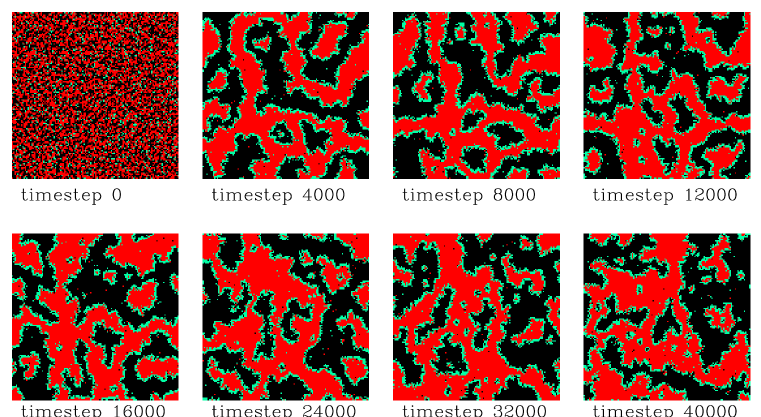
FIG. 2.: Time evolution of sponge microemulsion phase in absence of shear. The $x$ axis is along the horizontal and the $y$ axis along the vertical side of the simulation images shown here. The system size is $128\times 128$.

FIG. 3.: Time-averaged structure factor $S({\bf k},\tau)$ for sponge microemulsion case with no shear velocity. The system size is $128\times 128$. Values of $\tau$ depicted here are $8,000$ time steps on the left-hand side and $12,000$ time steps on the right. The axes on the right-hand figure are a mirror image of those on the left to aid visual clarity.

FIG. 4.: Time-averaged structure factor $S({\bf k},\tau)$ for sponge microemulsion case with no shear velocity. The system size is $128\times 128$. Values of $\tau$ depicted here are $28,000$ time steps on the left-hand side and $36,000$ time steps on the right. The axes on the right-hand figure are a mirror image of those on the left to aid visual clarity.

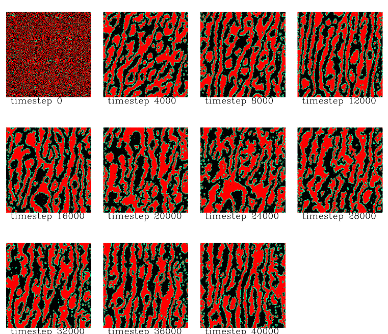
FIG. 5.: Time evolution of lamellar phase for a system size $256\times 256$ in the presence of shear. The $x$ axis is along the horizontal and the $y$ axis along the vertical side of the simulation images shown here. The imposed shear velocity is $\pm 0.2$ lattice units per time step in the $y$ direction, $+0.2$ being on the right.

FIG. 6.: Time-averaged structure factor $S({\bf k},\tau)$ for lamellar case with shear. The system size is $64\times 64$ and the shear velocity is $\pm 0.05$. Values of $\tau$ depicted here are $28,000$ time steps on the left-hand side and $36,000$ time steps on the right. The axes on the right-hand figure are a mirror image of those on the left to aid visual clarity.

FIG. 7.: Time-averaged structure factor $S({\bf k},\tau)$ for lamellar case with shear. The system size is $128\times 128$ and the shear velocity is $\pm 0.1$. Values of $\tau$ depicted here are $48,000$ time steps on the left-hand side and $56,000$ time steps on the right. The axes on the right-hand figure are a mirror image of those on the left to aid visual clarity.

FIG. 8.: Time-averaged structure factor $S({\bf k},\tau)$ for lamellar case with shear. The system size is $256\times 256$ and the shear velocity is $\pm 0.2$. Values of $\tau$ depicted here are $40,000$ time steps on the left-hand side and $48,000$ time steps on the right. The axes on the right-hand figure are a mirror image of those on the left to aid visual clarity.

FIG. 9.: Time averaged structure factor at $k_{y}=0.0$ for system sizes $N=64$ (solid line), $N=128$ (dashed line) and $N=256$ (dotted line) plotted against $k_{x}$. The data is taken from the left-hand plots of Figures $6,7\&8$ respectively. Note that the shift in the position of the peak is due to the discretisation of the wave vectors (compare discussion in Sec. III.B.)

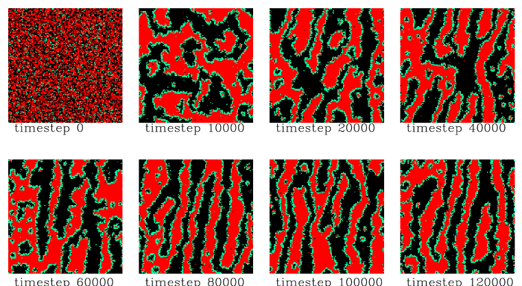
FIG. 10.: Time evolution of ternary amphiphilic system, shear imposed only after time step $10,000$. The $x$ axis is along the horizontal and the $y$ axis along the vertical side of the simulation images shown here. The imposed shear velocity is $\pm 0.1$ lattice units per time step in the $y$ direction, $+0.1$ being on the right. The system size is $128\times 128$.

FIG. 11.: Time-averaged structure factor $S({\bf k},\tau)$ for the case with shear imposed only after $10,000$ time steps. The system size is $128\times 128$ and the shear velocity is $\pm 0.1$. Values of $\tau$ depicted here are $10,000$ time steps on the left-hand side and $120,000$ time steps on the right. The axes on the right-hand figure are a mirror image of those on the left to aid visual clarity.

Time Step	$X^{2}$	$Y^{2}$	$X^{2}$:$Y^{2}$
0	6148$\pm$ 68	6147$\pm$ 52	1.000$\pm$ 0.014
4000	6081$\pm$ 144	6214$\pm$ 166	0.979$\pm$ 0.035
8000	6046$\pm$ 33	6249$\pm$ 91	0.968$\pm$ 0.015
12000	6161$\pm$ 137	6134$\pm$ 143	1.005$\pm$ 0.033
16000	6129$\pm$ 160	6166$\pm$ 152	0.994$\pm$ 0.036
20000	6169$\pm$ 103	6126$\pm$ 92	1.007$\pm$ 0.023
24000	6148$\pm$ 144	6147$\pm$ 169	1.000$\pm$ 0.036
28000	6135$\pm$ 150	6160$\pm$ 155	0.996$\pm$ 0.035
32000	6150$\pm$ 101	6145$\pm$ 103	1.001$\pm$ 0.024
36000	6113$\pm$ 56	6182$\pm$ 93	0.989$\pm$ 0.017
40000	6107$\pm$ 147	6188$\pm$ 155	0.987$\pm$ 0.034

TABLE I.: Total $X$ and $Y$ component values of surfactant dipole vectors at selected time steps for the case of no shear and $N=128$. The ratio $X^{2}$:$Y^{2}$ is also shown. The error bars result from ensemble averaging over five independent runs.

Time Step	$X^{2}$	$Y^{2}$	$X^{2}$:$Y^{2}$
0	6163$\pm$ 77	6152$\pm$ 51	1.001$\pm$ 0.015
4000	7248$\pm$ 276	5068$\pm$ 234	1.430$\pm$ 0.086
8000	7647$\pm$ 218	4669$\pm$ 229	1.638$\pm$ 0.093
12000	7320$\pm$ 136	4996$\pm$ 168	1.465$\pm$ 0.056
16000	7348$\pm$ 184	4968$\pm$ 238	1.479$\pm$ 0.080
20000	7120$\pm$ 253	5196$\pm$ 319	1.370$\pm$ 0.097
24000	7120$\pm$ 193	5196$\pm$ 221	1.370$\pm$ 0.069
28000	7083$\pm$ 195	5232$\pm$ 225	1.354$\pm$ 0.069
32000	7310$\pm$ 100	5006$\pm$ 149	1.460$\pm$ 0.048
36000	7060$\pm$ 125	5256$\pm$ 200	1.343$\pm$ 0.056
40000	7211$\pm$ 132	5105$\pm$ 219	1.412$\pm$ 0.066

TABLE II.: Total $X$ and $Y$ component values of surfactant dipole vectors at selected time steps for the case of shear flow and $N=128$. The ratio $X^{2}$:$Y^{2}$ is also shown. The error bars are obtained from averaging over five independent runs.

REFERENCES

- [1] Hoffmann H., Adv. Mater. 6 (1994) 116-129.
- [2] Boghosian B.M., Coveney P.V. and Emerton A.N., Proc. Roy. Soc. Lond. A. 452 (1996) 1221-1250.
- [3] Koppi K.A., Tirrell M. and Bates F.S., Phys. Rev. Lett. 70 (1993) 1449-1452.
- [4] Yamamoto J. and Tanaka H., Phys. Rev. Lett. 77 (1996) 4390-4393.
- [5] Mahjoub H.F., McGrath K.M. and Kleman, M., Langmuir 12 (1996) 3131-3138.
- [6] Cates M.E. and Milner S.T., Phys. Rev. Lett. 62 (1989) 1856-1859.
- [7] Frisch U., Hasslacher B. and Pomeau Y., Phys. Rev. Lett. 56 (1986) 1505-1508.
- [8] Gunstensen A.K. and Rothman D.H., Physica D. 47 (1991) 47-52.
- [9] Rothman D.H. and Zaleski S., Rev. Mod. Phys. 66 (1994) 1417-1475.
- [10] Rothman D.H., Phys. Rev. Lett. 65 (1990) 3305-3308.
- [11] Olson J.F. and Rothman D.H., J. Stat. Phys. 81 (1995) 199-222.
- [12] Rothman D.H. and Keller J.M., J. Stat. Phys. 52 (1988) 1119-1127.
- [13] Emerton A.N., Coveney P.V. and Boghosian B.M., Phys. Rev. E. 55 (1997) 708-720.
- [14] Weig F.W.J., Coveney P.V. and Boghosian B.M., “Lattice-gas simulations of minority-phase domain growth in binary immiscible and ternary amphiphilic fluids” submitted to Phys. Rev. E. (1997).
- [15] Cates M.E., private communication (1996/97).
- [16] Boghosian B.M., Coveney P.V, unpublished.