Critical point shift in a fluid confined between opposing walls

Abstract

The properties of a fluid, or Ising magnet, confined in a $L\times\infty$ geometry with opposing surface fields at the walls is studied by density matrix renormalization techniques. In particular we focus on the effect of gravity on the system, which is modeled by a bulk field whose strength varies linearly with the distance from the walls. It is well known that in the absence of gravity phase coexistence is restricted to temperatures below the wetting temperature. We find that gravity restores phase coexistence up to the bulk critical temperature, in agreement with previous mean field results. A detailed study of the scaling to the critical point, as $L\to\infty$, is performed. The temperature shift scales as $1/L^{y_{T}}$, while the gravitational constant scales as $1/L^{1+y_{H}}$, with $y_{T}$ and $y_{H}$ the bulk thermal and magnetic exponents respectively. For weak surface fields and $L$ not too large, we also observe a regime where the gravitational constant scales as $1/L^{1+y_{H}-\Delta_{1}y_{T}}$ ($\Delta_{1}$ is the surface gap exponent) with a crossover, for sufficiently large $L$, to a scaling of type $1/L^{1+y_{H}}$.

I Introduction

The Ising model has played a central role in the theory of critical phenomena. It is simple enough that it can be studied in great detail (although exact solutions are restricted only to a few cases in two dimensions), and it can be used to model many interesting physical situations. The two phases with opposite magnetization, which coexist in an infinite system for temperatures lower than the bulk critical temperature $T_{c}$, can be thought as the two coexisting phases (liquid and vapor) of a simple fluid. Besides bulk critical phenomena, which occur in a system infinitely extended in all directions, much interest has been focused on the study of the critical behavior of confined systems, which are of finite extensions in one or more directions.

A few years ago Parry and Evans [1, 2], using a mean field Ginzburg-Landau approach, investigated the phase diagram of a $d$-dimensional Ising model in a $L\times\infty^{d-1}$ geometry, i.e. confined between two walls separated by a finite distance $L$. They considered opposing walls, where one wall favors the “liquid” and the other the “vapor” phase; in the Ising language this corresponds to introducing surface magnetic fields $h_{1}$ and $h_{2}$ with opposite sign ($h_{1}h_{2}<0$). It was found [1] that two phase coexistence is restricted to temperatures below the wetting temperature $T_{w}$; Brochard and de Gennes had come to a similar conclusion as well [3]. These results were later confirmed by extensive Monte Carlo simulations, both in two and three dimensions [4, 5, 6]. The two dimensional Ising model with opposing surface fields was recently solved exactly by Maciołek and Stecki [7] using transfer matrices and pfaffian techniques. The surprising characteristic of Parry and Evans’ results [1, 2] is that one does not seem to recover information about the bulk critical point when the limit $L\to\infty$ is taken: for all values of $L$ two phase coexistence is restricted to $T<T_{w}$.

In trying to clarify the remarkable properties of this system, Rogiers and Indekeu [8] introduced an extra bulk field which varies linearly with the distance from the walls and which plays the role of gravity in the fluid. They found, in a mean field analysis, that the competing effect of opposing surface fields and gravity restores phase coexistence up to the bulk critical temperature.

In the present paper we study the model of Rogiers and Indekeu at the lower critical dimension ($d=2$) and beyond the mean field approximation to test the validity of their conclusion when thermal fluctuations are properly taken into account. Our results are based on a density matrix renormalization group (DMRG) calculation and essentially confirm the mean field scenario. We also analyze the exponents describing the critical point shift along the thermal and gravitational field direction and compare our findings with some predictions due to scaling analysis [8, 9, 10, 11].

A brief report of this work has been presented in Ref. [12]; here we give a full account of our work and present a series of results concerning in particular the analysis of the finite size scaling of the gravitational constant for low surface fields, where interesting crossover phenomena take place. This paper is organized as follows. In Sec.II we introduce the model and in Sec.III briefly review the DMRG technique. In Sec.IV we compare DMRG results with exact ones in the absence of a gravitational field. In Sec.V we present the phase diagram as derived from DMRG calculations and discuss its main features. In Sec.VI we show some magnetization profiles and compare the DMRG results with those obtained by capillary wave theory. In Sec. VII we present some conclusions.

II Model

We consider a ferromagnetic Ising model in a $L\times\infty$ strip with the following Hamiltonian:

$$H=-J\sum_{i,j}s_{i,j}s_{i+1,j}-J\sum_{i,j}s_{i,j}s_{i,j+1}+h_{1}\sum_{j}s_{1,j}$$ (1)

$$-h_{1}\sum_{j}s_{L,j}+g\sum_{j}\sum_{i=1}^{L}(2i-1-L)s_{i,j},$$ (2)

where $J>0$, $s_{i,j}=\pm 1$, $-\infty<j<\infty$ and $1\leq i\leq L$. For simplicity we restrict ourselves to the case of surface fields of equal magnitude $|h_{1}|$. The last term of the right-hand side of Eq. (2) is a bulk field varying linearly with the distance from the walls, which, for convenience, is chosen antisymmetric with respect to the center of the strip. This field models the effect of gravity on a fluid and $g$ plays the role of the gravitational constant.

In the limit $g\to 0$ one recovers the models studied by Parry and Evans [1]; in two dimensions the wetting temperature $T_{w}$ is known exactly and satisfies the equation [13]

$$e^{a}\left[\cosh(a)-\cosh(b)\right]=\sinh(a),$$ (3)

where $a=2J/T_{w}$ and $b=2h_{1}/T_{w}$. For $h_{1}=0$ the wetting temperature $T_{w}$ is equal to the bulk critical temperature $T_{c}=2J/\ln(1+\sqrt{2})$. It decreases monotonically with $h_{1}$ and vanishes for $h_{1}=J$.

In the rest of the paper we will be primarily interested in the competing effect of surface fields and gravity; it is clear from the Hamiltonian (2) that these occur when $h_{1}$ and $g$ have the same sign.

III DMRG method

The density matrix renormalization group was introduced by White [14, 15] to study the ground state properties of quantum spin chains. The method is very accurate and it has been successfully applied to many one dimensional quantum problems (for a review see Ref. [16]).

Exploiting the relation between a $d$-dimensional quantum system and a $d+1$-classical system, Nishino [17] was able to extend the DMRG to two-dimensional classical systems. In this case White’s algorithm is applied to the construction of effective transfer matrices of large systems.

In a transfer matrix approach the partition function of a system defined on a $L\times\infty$ strip is equal to the largest eigenvalue of the so-called transfer matrix $T_{L}$ [18]. Numerical calculations are restricted to strips of small widths (typically $L<20$ for an Ising model) since the dimension of $T_{L}$ grows exponentially with the strip width.

In a DMRG calculation one starts from a transfer matrix of a small system that can be handled exactly. Using the information about the thermodynamics of this system one generates an effective transfer matrix of a larger system. The strip width grows at each DMRG iteration and the spin space is very efficiently truncated to keep the dimensionality of the effective transfer matrix controlled.

Figure 1 shows schematically a transfer matrix element generated by the DMRG algorithm. The matrix consists of block and spin variables indicated in the figure by rectangles and circles respectively. A block, whose states are labeled by a variable $\xi$ which can take $m$ possible values only, describes approximately a collection of spins.

FIG. 1.: Schematic view of a transfer matrix element of a strip of width $L$ generated by DMRG. $\xi$ and $s$ label block and spin variables respectively, with $\xi=1,2\ldots m$ and $s=\pm 1$. The total dimension of the matrix is $4m^{2}\times 4m^{2}$. The arrow denotes the transfer direction.

Obviously by allowing larger $m$ one obtains more accurate numerical results; in a typical DMRG calculation the accuracy grows very rapidly with $m$ [14]. In the present case we found that for strips up to $L=100$ a value of $m=40$ is sufficient to guarantee a very high accuracy of the numerical results. In our calculations we have used the finite system method described by White in Ref.[15], a version of the DMRG algorithm designed to accurately study finite size systems. For more details we refer readers to the existing literature (see Refs.[14, 15, 16, 17]).

Note that we use open boundary conditions: the blocks on the left and right side of Fig. 1 are not coupled together. Although it is possible to implement the DMRG method with periodic boundary conditions it turns out that the accuracy is lower than in the open boundary condition case [15]. Therefore the method is best suited to study properties of two dimensional classical systems in contact with walls or with free surfaces.

IV Zero-gravity case

In the limit $g\to 0$ the model described by the Hamiltonian (2) has been solved exactly [7]. In this section we summarize briefly some known facts and present results obtained from DMRG calculations.

For temperatures below a temperature $T_{d}(L)$, which Parry and Evans [1] interpreted as the critical temperature of the confined system, two phases coexist. Typical magnetization profiles are shown in Fig. 2(a). For $T_{d}(L)\leq T<T_{c}$ the system is in a single interface-like state as depicted in Fig. 2(b). For $L\to\infty$ $T_{d}(L)$ scales as [1]:

$$T_{d}(L)-T_{w}\sim L^{-1/\beta_{s}}.$$ (4)

Here $\beta_{s}$ is the exponent describing the divergence of the thickness of the wetting layer for a semi-infinite system with a surface field $h_{1}$: $l\sim(T_{w}-T)^{-\beta_{s}}$.

Swift et al. [19], who analyzed the same system from a different angle, interpreted $T_{d}(L)$ rather as a shifted wetting temperature, in contrast with the point of view of Ref.[1]. We will come back to this point again later.

FIG. 2.: Magnetization profiles for the model in absence of gravity in the two phase coexistence region for $0\leq T<T_{d}(L)$ (a) and in the single phase region for $T_{d}(L)\leq T<T_{c}$ (b). $m_{0}$ denotes the bulk magnetization of the Ising model.

We have calculated $T_{d}(L)$ from the correlation function between two neighboring spins at the center of the strip:

$$c_{L/2}=\langle s_{\frac{L}{2},j}s_{\frac{L}{2}+1,j}\rangle.$$ (5)

In the two phase coexistence region $c_{L/2}$ is large and positive since the two spins are preferably aligned. If an interface is present, $c_{L/2}$ drops to smaller values, since in many configurations when the interface is located at the center of the strip the two spins tend to have opposite values. We identify $T_{d}(L)$ as the maximum of the temperature derivative of $c_{L/2}$. There is obviously no sharp phase transition on an $L\times\infty$ system and in the present case $T_{d}(L)$ corresponds to a pseudocritical point.

As $L\to\infty$, $T_{d}(L)$ scales as (4) towards the wetting temperature, with the two dimensional wetting exponent $\beta_{s}=1$ [13]. Figure 3 shows a plot of $T_{d}(L)$ vs $1/L$ for various values of the surface field $h_{1}$. On the vertical axis the exact values of the wetting temperatures $T_{w}(h_{1})$, derived from Eq. (3), are shown. As can be seen from the figure the scaling behavior of $T_{d}(L)$ is in good agreement with Eq. (4).

FIG. 3.: Plot of $T_{d}(L)$ vs $1/L$ for $J=1$ and various values of the surface field $h_{1}$. The crosses on the vertical axis are the values of the wetting temperatures derived from Eq.(3) where the data points are expected to scale to for $L\to\infty$.

The shift of $T_{d}(L)$ as $L\to\infty$ was also investigated in Monte Carlo simulations by Albano et al. [4]. They also found good agreement with (4).

Table I shows a comparison between the values of the wetting temperatures extrapolated from a finite size scaling of the DMRG data for $T_{d}(L)$ and the exact values given by Eq. (3); the agreement is up to the fourth decimal digit. We stress that the relevant source of errors for $T_{d}(L)$ is in the calculation of the numerical derivative of $c_{L/2}$; DMRG calculations provide values of $c_{L/2}$ which are very accurate.

TABLE I.: Comparison between DMRG data and exact values of the wetting temperatures $T_{w}$ for different values of the surface field $h_{1}$. The number between parenthesis are the error on the last two digits of the DMRG results.

$h_{1}$	$0.1$	$0.5$	$0.7$	$0.9$	$0.99$
DMRG	$2.25761(77)$	$1.95814(77)$	$1.63532(77)$	$1.10753(77)$	$0.58848(77)$
Exact [13]	$2.25710$	$1.95845$	$1.63496$	$1.10745$	$0.58845$

V Effect of gravity

It is convenient, before discussing the full phase diagram of the system described by the Hamiltonian (2) to focus on its ground state properties. The two states with all spins positive or negative are degenerate, with an energy per spin equal to:

$$\epsilon_{o}=-\left(2-\frac{1}{L}\right)J.$$ (6)

If $g$ is large and positive the ground state configuration is:

$$s_{i,j}=\left\{\begin{array}[]{cl}+1&\,\,\,{\mbox{i}f}\,\,\,1\leq i\leq\frac{L}{2}\\ &\\ -1&\,\,\,{\mbox{i}f}\,\,\,\frac{L}{2}+1\leq i\leq L,\end{array}\right.$$ (10)

with an energy per spin equal to:

$$\epsilon_{+-}=-\left(2-\frac{3}{L}\right)J+\frac{2h_{1}}{L}-\frac{gL}{2}.$$ (11)

Alternatively, if $g$ is large and negative the ground state has all spins reversed with respect to the configuration (10); in this case the energy is

$$\epsilon_{-+}=-\left(2-\frac{3}{L}\right)J-\frac{2h_{1}}{L}+\frac{gL}{2}.$$ (12)

The ground state is thus double degenerate if $\epsilon_{o}<\epsilon_{+-}$ and $\epsilon_{o}<\epsilon_{-+}$, which yields the following condition:

$$\frac{4(h_{1}-J)}{L^{2}}\,\,\,<\,\,g\,\,<\,\,\,\frac{4(h_{1}+J)}{L^{2}}$$ (13)

At $T=0$ the two phase coexistence region shrinks as $1/L^{2}$ towards the $g=0$ axis. The previous calculation is valid only for $h_{1}<J$; if the surface field is larger than $J$ (this implies also $T_{w}=0$) the range of values of $g$ for which one has phase coexistence at $T=0$ is given by:

$$0\,\,\,<\,\,g\,\,<\,\,\,\frac{4(h_{1}+J)}{L^{2}}.$$ (14)

In the rest of the paper we will consider only the case $h_{1}<J$.

The phase diagram of the model in a $(g,T)$ plane for $h_{1}=0.5$, $J=1$ is shown in Fig. 4. The curves indicate the phase boundaries between the two phase coexistence region (area below the curves) and a single phase region (above) for different values of the strip width $L$ [20]. When continued down to $T=0$ the phase boundaries meet the horizontal axis at the values of $g$ equal to the extremes of the interval (13).

The phase boundaries cross the axis $g=0$ at the interface delocalization temperatures $T_{d}(L)$ (indicated by horizontal arrows in Fig. 4), which scale to the wetting temperature $T_{w}$, indicated by a cross on the $g=0$ axis of Fig. 4. The striking feature of the phase diagram [8] is that for non-zero gravity phase coexistence extends at higher temperatures with respect to the case $g=0$ due to the competing effect of surface and gravitational fields. At negative $g$ the two phase coexistence is suppressed at lower temperatures than for $g=0$, since in this case gravity enhances the effect of the surface fields.

The phase boundary maxima [$g_{\rm max}(L)$,$T_{\rm max}(L)$], indicated by the vertical arrows in Fig. 4, shift towards the bulk critical point $T=T_{c}$, $g=0$ and can be identified as the finite system (pseudo) critical points. As $L\to\infty$ the whole critical region shifts towards the $g=0$ axis. This is in agreement with the results of Van Leeuwen and Sengers [11] who pointed out that in presence of gravity there is no criticality in an infinitely extended system.

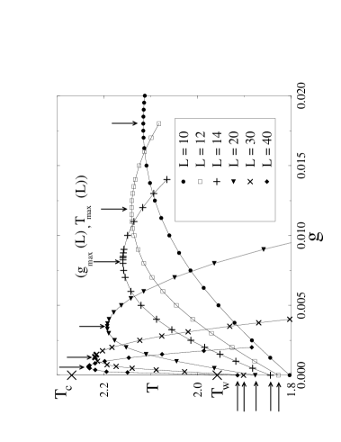
FIG. 4.: Phase diagram of the model in the $(g,T)$ plane. The curves are the phase boundaries between the two phase coexistence and the single phase regions for different values of the strip width. Notice the scaling to the wetting temperature (horizontal arrows) and to the critical point (vertical arrows).

The phase diagram of Fig. 4 is in agreement with the mean field results of Rogiers and Indekeu [8], who, in addition, found tricritical points located in the phase boundaries, which separate continuous from first order transition lines. Obviously these features are not found in two dimensions where the wetting transition is always critical, but they should be found in three dimensions where the wetting tricritical point is at $T>0$.

Finite size scaling [8, 9, 10, 11] predicts that the critical point shifts as follows:

$$T_{\rm max}(L)-T_{c}\sim L^{-y_{T}},$$ (15)

$$g_{\rm max}(L)\sim L^{-(1+y_{H})}.$$ (16)

$y_{T}$ and $y_{H}$ are the thermal and magnetic exponents of the Ising model, which in two dimensions are $y_{T}=1$ and $y_{H}=15/8$.

TABLE II.: The values of the extrapolated critical temperature from the scaling analysis of $T_{\rm max}(L)$ for different values of the surface field $h_{1}$, when $h_{1}<J$. The exact value is $T_{c}=2.269185\ldots$

$h_{1}$	$0.1$	$0.5$	$0.99$
DMRG	$2.269(3)$	$2.272(3)$	$2.271(3)$

In deriving Eq. (16) one assumes, as done by van Leeuwen and Sengers [11], that the gravitational constant $g$ times a length scales as a bulk constant field. This relates the scaling of $g$ to the bulk magnetic exponent $y_{H}$.

The DMRG data for $T_{\rm max}(L)$ are in very good agreement with the scaling relation (15), as shown in Fig. 5. Table II shows the values of $T_{c}$ extrapolated from the finite size scaling analysis of $T_{\rm max}(L)$ by means of iterated fits. Results are in good agreement with the exact value.

FIG. 5.: Scaling of $T_{\rm max}(L)-c$ vs $1/L$ for different surface fields. To avoid overlapping of data the values of $T_{\rm max}(L)$ have been shifted by a constant $c$, with $c=0$ for $h_{1}=0.1$, $c=0.3$ for $h_{1}=0.5$ and $c=0.6$ for $h_{1}=0.99$. Dotted lines are linear fits of the data points.

The finite size scaling along the gravitational field direction is more intriguing. Figure 6 shows a plot of $\ln[g_{\rm max}(L)]$ vs $\ln(L)$ for $h_{1}=0.5$ and $h_{1}=0.99$. In both cases there is agreement with the scaling relation (16): as $L$ grows the data points approach the dashed lines which have slope $-2.875$ (the value of the exponent $-1-y_{H}$ for the two dimensional Ising model). Notice that for $h_{1}=0.99$ the asymptotic behavior sets in already for $L\geq L_{0}\approx 20$ while for $h_{1}=0.5$ this happens only for $L\geq L_{0}\approx 60$.

The scaling behavior of $g_{\rm max}(L)$ for smaller surface fields is shown in Fig. 7; in this case the deviation from the expected exponents is so strong that one concludes that either (16) does not hold for small $h_{1}$ or the asymptotic behavior sets in only for strip widths much larger than those analyzed.

Following Fisher and Nakanishi [9, 10] who investigated the critical point shift in an Ising model confined between identical walls, one expects a scaling of $g_{\rm max}(L)$ of the type:

$$g_{\rm max}(L)=L^{-(1+y_{H})}\,\,\,\Omega\left(h_{1}L^{\Delta_{1}y_{T}}\right),$$ (17)

where $\Omega(x)$ is a scaling function and $\Delta_{1}$ the surface gap exponent (recall that $\Delta_{1}=1/2$ for the two-dimensional Ising model). The fact that the surface field enters in the form of a scaling variable $h_{1}L^{\Delta_{1}y_{T}}$ is a direct consequence of the scaling form of the singular part of the surface free energy [9, 10].

For $L\to\infty$ one should recover from (17) the scaling relation (16), which implies that:

$$\lim_{x\to\infty}\Omega(x)=\Omega_{\infty}\neq 0$$ (18)

When $h_{1}$ is sufficiently large and for not too small values of $L$, the scaling function in (17) can be replaced by its asymptotic value $\Omega_{\infty}$. In this limit, which we refer to as the saturated regime, $g_{\rm max}(L)$ becomes practically independent of $h_{1}$.

FIG. 6.: Plot of $\ln[g_{\rm max}(L)]$ vs $\ln L$ for $h_{1}=0.5$ (left) and $h_{1}=0.99$ (right). Error bars are smaller than symbol sizes. The dashed lines correspond to a slope $-2.875$ and are drawn as a guide to the eye.

From the analysis of the numerical data for $h_{1}=0.99$ one finds that $\Omega(x)$ saturates for $x>x_{0}\approx\sqrt{20}$. Consequently, for $h_{1}=0.5$, $0.2$ and $0.1$ the saturated regime is expected to occur for $L>L_{0}\approx 80$, $L>L_{0}\approx 500$ and $L>L_{0}\approx 2000$ respectively. Notice that a saturation value of $L_{0}\approx 80$ for $h_{1}=0.5$ is in agreement with our numerical data. Strips of width $L=500$ or $L=2000$ are beyond the possibilities of our numerical investigation; actually, calculations for $L>100$ (the largest size analyzed in the present work) are feasible, but for such large systems the value of $g_{\rm max}(L)$ is very small and affected by large relative error bars that make the scaling analysis difficult.

For $h_{1}=0$ one has $g_{\rm max}(L)=0$ since the phase boundaries of Fig. 4 become symmetric with respect to the $g=0$ axis. For very small surface fields one expects that $g_{\rm max}(L)$ scales linearly with $h_{1}$ [21]; this implies that:

$$\Omega(x)\sim x\hskip 28.45274pt{\mbox{\rm for}}\,\,\,x\to 0.$$ (19)

Therefore, in the strongly “undersaturated” regime, where $x=h_{1}L^{\Delta_{1}y_{T}}\ll\sqrt{20}$, one expects a scaling behavior in $L$ of the type:

$$g_{\rm max}(L)\sim L^{-(1+y_{H}-\Delta_{1}y_{T})}$$ (20)

In Fig. 7 the dashed-dotted lines have slopes equal to $-2.375$, which is the value of the exponent $-1-y_{H}+\Delta_{1}y_{T}$ for the two dimensional Ising model. As can be seen from the figure the numerical data are in good agreement with a scaling of type (20).

FIG. 7.: As in Fig. 6 for $h_{1}=0.1$ (left) and $h_{1}=0.2$ (right). Dashed and dashed-dotted lines have slopes $-2.875$ and $-2.375$ respectively.

We stress that (20) is not the asymptotic behavior of $g_{\rm max}(L)$ as $L\to\infty$, since for sufficiently large $L$ the scaling is of type (16). To verify this we have calculated $g_{\rm max}(L)$ for different strip widths at constant values of $x=h_{1}L^{\Delta_{1}y_{T}}$. The data points are shown in Fig. 8 and they are calculated in the undersaturated regime ($x<x_{0}\approx\sqrt{20}$); the agreement with the exponent $1+y_{H}=2.875$ is very good.

To conclude this section we point out that also for the temperature one expects a shift of the type [9, 10]:

$$T_{c}-T_{\rm max}(L)=L^{-y_{T}}\,\,\Gamma(h_{1}L^{\Delta_{1}y_{T}}).$$ (21)

Nakanishi and Fisher [10] analyzed the behavior of $\Gamma(x)$ in a mean field model confined between identical walls and found that $\Gamma(x)$ depends very weakly on its argument $x$. This is also found in the present study, as it can be seen from the fact that (1) the slopes of the data points of Fig. 5 are almost equal, i.e. they do not depend sensibly on the value of the surface field, and (2) the points are very well fitted by straight lines.

FIG. 8.: Plot of $\ln[g_{\rm max}(L)]$ vs $\ln L$ at constant values of $x=h_{1}L^{\Delta_{1}y_{T}}$. The data correspond to (a) $x={\sqrt{10}}$ and (b) $x={\sqrt{0.4}}$. Dashed lines have slope ${-2.875}$.

VI Magnetization Profiles

Figures 9 and 10 show some examples of magnetization profiles calculated by DMRG for various values of the gravitational constant and temperatures. The profiles (a) refer to points below the phase boundaries of Fig. 4, i.e. in the two phase coexistence region. The two coexisting phases are expected to have magnetization profiles similar to those depicted in Fig. 2(a); the profiles (a) are actually the result of the average over the two phases.

The magnetization in the two phase coexistence region does not decay to a bulk constant value far from the walls as in Fig. 2(a). The inset of Fig. 9 shows an enlargement of the profile (a) at the center of the strip: due to the presence of gravity the profile follows a straight slightly inclined line. We stress that the accuracy of the DMRG results for the magnetization profiles is very high, so error bars are much smaller than symbol sizes also in the scale of the inset of Fig. 9.

In the single phase region (Figs. 9,10 (b,c)) the system develops an interface: gravity has the tendency to localize the interface at the center of the strip in a configuration of minimal energy. The larger the value of $|g|$ the stronger the localization effect, as it can be seen in the figures: the profiles (b) correspond to a value of the gravitational constant $7.5$ times larger than the profiles (c). Notice also in the profiles (b) the competing effect of surface fields and gravity which is visible in the vicinity of the walls.

The dashed lines of Figs. 9-10 are the magnetization profiles predicted by the capillary wave theory, which are derived in the Appendix and are given by:

$$m(l)=\frac{2m_{0}}{\sqrt{\pi}}\int_{0}^{l/\xi_{\perp}}dt\,e^{-t^{2}},$$ (22)

Here $2\xi_{\perp}$ is the average interfacial width and $m_{0}$ is the bulk magnetization of the Ising model in absence of gravity. All the parameters appearing in (22) are known exactly, and the dashed lines of Fig. 9, 10 are not the results of a fitting.

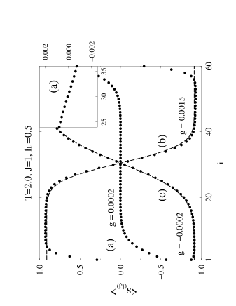
FIG. 9.: Magnetization profiles at a fixed temperature $T=2.0$ and for three different values of the gravitational constants calculated by DMRG (filled circles). The profile (a) is in two phase coexistence region. (b) and (c) are profiles in the single phase region situated to the left and to the right of the two phase coexistence region of Fig. 4 respectively. The dashed lines are the result of the capillary wave theory calculation as given by (22). Inset: enlargement of the profile (a) in the center of the strip.

FIG. 10.: As in Fig. 9 at higher temperature ($T=2.1$). Notice that the discrepancy between the profiles in the interfacial region ((b) and (c)) and those predicted by the capillary wave theory increase at higher temperatures. Inset: enlargement of the profile (b) in the vicinity of one wall.

Capillary wave theory profiles agree very well with the DMRG results especially at low temperatures where the approximations introduced are very good. Eq. (22) is valid in the limit $\xi_{\perp}\ll L$ where the effects of the walls can be neglected. This condition is satisfied at low temperatures and at not too small values of $|g|$. Notice also that if $|g|$ is too large the magnetization profile (22) far from the interfacial region differs sensibly from the DMRG results, since the effect of gravity in that region has been neglected. This can be seen more clearly in the inset of Fig. 10.

VII Conclusions

In this article we have studied the critical behavior of an Ising model confined between opposing walls and subject to a bulk “gravitational” field. The competing effects of surface and bulk fields restore phase coexistence up to the bulk critical temperature, in agreement with the results of a mean field study of the model [8]. The strong thermal fluctuations in two dimensions do not affect the mean field results, which a fortiori should also be valid in three dimensions where fluctuation effects are weaker.

Wetting plays an important role in the model as it was found in the studies in the absence of gravity [1, 2, 3]. However, limiting the analysis to $g=0$ causes us to miss much of the interesting physics that arises when gravity is included. In particular, one misses the critical point of the confined system [8], which we have identified with [$g_{\rm max}(L)$,$T_{\rm max}(L)$], the maximum of the phase boundaries separating the two-phase coexistence from the single phase regions.

We have performed a detailed analysis of the critical point shift as $L\to\infty$ and found that temperature and gravitational constant scale in agreement with previous finite size scaling hypothesis [8, 9, 10, 11]. Along the gravitational field direction in the limit of small surface fields a crossover behavior between two different scaling regimes is found.

This limit has been considered recently in studies of critical adsorption [22, 23]. Desai et al. [22] in a experiment on a binary liquid mixture were able to investigate the weak surface field regime by chemically modifying the surface of the solid substrate which is in contact with the liquid. They found an unexpected behavior of the adsorption for small surface fields, in possible disagreement with scaling theory. This issue was discussed recently also by Ciach et al. [23]. In general we expect interesting physics to arise in the limit $h_{1}\to 0$ due to the interplay between bulk and surface criticality, as we found in the analysis of the scaling behavior of the gravitational constant for the model studied in this article.

Acknowledgments - It is a pleasure to thank C.J. Boulter, R. Dekeyser, M.S.L. du Croo de Jongh, C. Franck, J.O. Indekeu, J.M.J. van Leeuwen, A.O. Parry and J. Rogiers for stimulating discussions. We acknowledge also fruitful correspondence with A. Maciołek and J. Stecki. E.C. would like to thank J. Sznajd for the kind hospitality during his visit to the Institute for Low Temperature and Structure Research of the Polish Academy of Sciences (Wrocław) where part of this work was done. A.D. is grateful to R. Dekeyser for financial support during his visit at the Institute for Theoretical Physics of the Catholic University of Leuven. E.C. is financially supported by KULeuven Research Fund F/96/20.

Appendix: Capillary-wave theory

In capillary wave theory [24] one assumes that a sharp interface separates two regions of constant magnetization. We take magnetizations equal to $\pm m_{0}$, the bulk magnetization of the Ising model in absence of external fields, which is known exactly. In this approximation gravity does not affect the magnetization far from the interfacial region and bulk fluctuations are neglected. In the continuum limit the interface is described by a single valued function $l(y)$ where $y$ is the coordinate along the wall ($-\infty<y<\infty$) and $l$ denotes the displacement of the interface from the center of the strip (see Fig. 11). This is a solid-on-solid (SOS) approximation where overhangs are neglected [25].

The continuum Hamiltonian is given by:

$$H\left[l(y)\right] = \int_{-\infty}^{+\infty}dy\,\,\left\{\frac{\sigma_{0}}{2}\left(\frac{dl}{dy}\right)^{2}+U(l)\right\}$$ (23)

where $\sigma_{0}$ is the surface tension and $U(l)$ the potential acting on the interface. The partition function is given by:

$$Z=\int{\cal{D}}l(y)\,\,e^{-\beta H[l(y)]}$$ (24)

where $\beta$ denotes the inverse temperature. In (24) we integrate over all the possible interface shapes described by single valued functions. Due to well-known relations between path integrals and quantum mechanics [26], the previous problem can be mapped into a one dimensional quantum problem which consists in solving the following Schrödinger equation:

$$\left(-\frac{1}{2\sigma_{0}\beta^{2}}\frac{d^{2}}{dl^{2}}+U(l)\right)\psi_{n}(l)=E_{n}\psi_{n}(l)$$ (25)

The ground state wave function squared $|\psi_{0}(l)|^{2}$ denotes the probability of finding the interface at a position $l$. The potential has the following form:

$$U(l;L)=W(l;L)+V_{g}(l)$$ (26)

Here $W(l;L)$ is the confining potential due to the presence of the walls:

$$W(l;L)=\left\{\begin{array}[]{cc}0&\mbox{if}\,\,|l|\leq L/2\\ &\\ +\infty&\mbox{if}\,\,|l|>L/2\end{array}\right.$$ (30)

$V_{g}(l)$ represents the contribution of gravity to the interfacial potential and can be calculated from the microscopic Hamiltonian (2). If the interface is located between the k-th and (k+1)-th spin of the system gravity gives the following contribution to the energy:

$$Q(k) = gm_{0}\left\{\sum_{i=1}^{k}(2i-1-L)-\sum_{i=k+1}^{L}(2i-1-L)\right\}$$ (31)

$$= 2m_{0}gk(k-L)$$ (32)

Shifting appropriately the origin of the coordinates one finds:

$$V_{g}(l) = 2m_{0}gl^{2}+c$$ (33)

where $c$ is a constant.

FIG. 11.: Example of an interfacial configuration described by a continuous single-valued function $l(y)$ as in the solid-on-solid approximation. All the spins at the two sides of the interface are fixed and equal to $\pm m_{0}$. The arrows denote the elastic force that tends to bring the interface in its equilibrium position.

Neglecting the effect of the confining potential (30) becomes the Schrödinger equation for a harmonic oscillator, with ground state wave function equal to:

$$\psi_{0}(l) = \frac{e^{-l^{2}/(2\xi_{\perp}^{2})}}{\pi^{1/4}\sqrt{\xi_{\perp}}}.$$ (34)

$\xi_{\perp}$ denotes the interfacial width:

$$\xi_{\perp}=\sqrt{\frac{T}{2\sqrt{|g|m_{0}\sigma_{0}}}}.$$ (35)

Here $m_{0}$ is the bulk magnetization and $\sigma_{0}$ is the surface tension which are known exactly for the $d=2$ Ising model at $g=0$. The analysis is valid for $\xi_{\perp}\ll L$ where the probability of finding the particle outside the walls is negligible and the confining potential $W(l;L)$ can be ignored.

From (34) one can easily calculate the magnetization profile as function of the distance from the center of the strip $l$:

$$m(l)=m_{0}\left\{\int_{-\infty}^{l}ds\,\,\left|\psi_{0}(s)\right|^{2}-\int_{l}^{+\infty}ds\,\,\left|\psi_{0}(s)\right|^{2}\right\}$$ (36)

which yields the result given in (22).

REFERENCES

- [1] A. O. Parry and R. Evans, Phys. Rev. Lett. 64, 439 (1990).
- [2] A. O. Parry and R. Evans, Physica 181 A, 250 (1992).
- [3] F. Brochard-Wyart and P. G. de Gennes, C. R. Acad. Sci. Paris II 297, 223 (1983).
- [4] E. V. Albano, K. Binder, D.W. Heermann and W. Paul, Surf. Sci. 223, 151 (1989).
- [5] E. V. Albano, K. Binder, D.W. Heermann and W. Paul, J. Chem. Phys. 91, 3700 (1989).
- [6] K. Binder, D. P. Landau and A. M. Ferrenberg, Phys. Rev. Lett. 74, 298 (1995); Phys. Rev. E 51, 2823 (1995).
- [7] A. Maciołek and J. Stecki, Phys. Rev. B 54, 1128 (1996).
- [8] J. Rogiers and J. O. Indekeu, Europhys. Lett. 24, 21 (1993).
- [9] M. E. Fisher and H. Nakanishi, J. Chem. Physics 75, 5857 (1981).
- [10] H. Nakanishi and M. E. Fisher, J. Chem. Physics 78, 3279 (1983).
- [11] J. M. J. van Leeuwen and J. V. Sengers, Physica 128 A, 99 (1984); Physica 138 A, 1 (1986).
- [12] E. Carlon and A. Drzewiński, Phys. Rev. Lett.79, 1591 (1997).
- [13] D. B. Abraham, Phys. Rev. Lett.44, 1165 (1980).
- [14] S. R. White, Phys. Rev. Lett.69, 2863 (1992).
- [15] S. R. White, Phys. Rev. B 48, 10345 (1993).
- [16] For a review of the DMRG method and some of its applications for one dimensional quantum systems see: G. A. Gehring, R. J. Bursill, T. Xiang, Act. Phys. Pol. A 91, 105 (1997); cond-mat/9705128.
- [17] T. Nishino, J. Phys. Soc. Jpn. 64, 3598 (1995).
- [18] For more details about transfer matrices see, for instance, R. J. Baxter, Exactly Solved Models in Statistical Mechanics, Academic Press 1982.
- [19] M. R. Swift, A. L. Owczarek and J. O. Indekeu, Europhys. Lett. 14, 475 (1991); J. O. Indekeu, M. R. Swift and A. L. Owczarek, Phys. Rev. Lett.66, 2174 (1996).
- [20] The phase boundaries have been calculated with the same method that has been used for the calculation of : at fixed we identified the phase boundaries with the maximum of the temperature derivative of .
- [21] Fisher and Nakanishi [9] argued that it is plausible to expect a linear scaling of the critical bulk field as function of , for small in the case of confinement between identical walls.
- [22] N. S. Desai, S. Peach and C. Franck, Phys. Rev. E52 4129 (1995).
- [23] A. Ciach, A. Maciołek and J. Stecki, submitted to J. Chem. Phys.
- [24] J. S. Rowlinson and B. Widom, Molecular Theory of Capillarity, Clarendon Press, Oxford 1982.
- [25] J. Stecki, Phys. Rev. B47, 7519 (1993); J. Stecki, A. Maciołek and K. Olaussen, Phys. Rev. B49, 1092 (1993).
- [26] D. M. Kroll and R. Lipowski,Phys. Rev. B28, 5273 (1983).