Universal scaling behavior of coupled chains of interacting fermions

Abstract

The single-particle hopping between two chains is investigated by exact-diagonalizations techniques supplemented by finite-size scaling analysis. In the case of two coupled strongly-correlated chains of spinless fermions, the Taylor expansion of the expectation value of the single-particle interchain hopping operator of an electron at momentum $k_{F}$ in powers of the interchain hopping $t_{\perp}$ is shown to become unstable in the thermodynamic limit. In the regime $\alpha<\alpha_{2p}$ ($\alpha_{2p}\simeq 0.41$) where transverse two-particle hopping is less relevant than single-particle hopping, the finite-size effects can be described in terms of a universal scaling function. From this analysis it is found that the single-particle transverse hopping behaves as $t_{\perp}^{\alpha/(1-\alpha)}$ in agreement with a RPA-like treatment of the interchain coupling. For $\alpha>\alpha_{2p}$, the scaling law is proven to change its functional form, thus signaling, for the first time numerically, the onset of coherent transverse two-particle hopping.

]

The physical nature of a system of coupled chains of strongly-correlated fermions is currently a very controversial issue. Such a problem has motivated lots of efforts in the recent past, both theoretically and experimentally, for a number of fundamental reasons. First, a better knowledge of this system will provide further insights to understand the dimensional cross-over from one dimension ($1D$) to two dimensions ($2D$) [1]. Secondly, strictly $1D$ chains have a very peculiar generic physical behavior known as the Luttinger Liquid (LL) behavior and it is essential to know how stable the LL is with respect to small perturbations such as the interchain hopping. Moreover, it is not clear yet under which experimental conditions the LL behavior can be observed experimentally.

Some time ago, Anderson suggested [2] that the effect of the interchain hopping may be strongly affected by the $1D$ character of each chain. It was conjectured that an intrachain repulsion of intermediate strength might be sufficient to lead to a confinement of the particles within each chain. Anderson’s confinement scenario has received much interest since such a mechanism could explain the anomalous transverse transport [3] observed for instance in quasi one-dimensional compounds such as the organic superconductors [4, 5].

The LL generic behavior of a $1D$ interacting electrons chain [6] differs radically from that of a Fermi liquid. First, there are no quasiparticle-like excitations but rather collective modes with different velocities for spin and charge (spin-charge separation). This leads to the absence of a step in the momentum distribution at the Fermi level but rather to a singularity of the form $n(k)-n(k_{F})\sim|k-k_{F}|^{\alpha}\,\text{sign}(k_{F}-k)$. It is remarkable that the exponent $\alpha$ is the only parameter which determines completely the low-energy properties of a spinless LL. In particular, all the exponents of the static and dynamical correlation functions are simply related to $\alpha$ (with given sign of the interaction). We shall then consider $\alpha$ as the key parameter fully determining the important properties of the $1D$ metallic system.

The central issue we shall focus on in the following study is the physical role of a small interchain hopping $t_{\perp}$. Such a question has been addressed by several authors using different methods and various concepts have emerged from these studies such as the notion of relevance/irrelevance in the Renormalization Group (RG) sense or the concept of coherence/incoherence.

Simple RG calculations [7, 8] suggest that the transverse hopping is a relevant perturbation for $\alpha<1$. In that case, the system flows towards a strong-coupling fixed point which can not be determined. On the other hand, for $\alpha>1$, the hopping becomes irrelevant and can in principle be neglected. This approach, however, has some limitations. First, it is a perturbative method limited to first order in $t_{\perp}$ and there is no guaranty that this should work for such a problem. Secondly, even when irrelevant, the hopping term always generates new and relevant interchain two-particles hopping for all values of the LL parameter $\alpha$ [8, 9]. As a consequence, the system always flows to strong coupling and, thus, it seems hazardous to make predictions about the true ground state based only upon the RG arguments.

Another approach to this problem takes advantage of a mapping of the two-chain system onto a two-level system coupled to a bath of oscillators [10]. This study suggests that relevance itself is not a sufficient condition to cause coherent motion between the chains. The notion of coherence has been explained in simple terms by Anderson and coworkers [10] by assuming a system of two separate chains prepared at time $t=0$ with a different number of particles. Then, if the interchain hopping is switched on, one can consider the probability $P(t)$ of the system returning to its initial state after a time $t$. Coherence or incoherence can then be simply defined as the presence or absence of oscillations in $P(t)$. This treatment suggests the existence of two different regimes: for $\alpha<\alpha_{0}$, where $\alpha_{0}$ depends on $t_{\perp}$ and is always smaller than $1/2$, coherent motion between the chains takes place while this motion becomes incoherent for $\alpha>\alpha_{0}$. It is argued that, since the interchain hopping is treated as a perturbation, this result can be applied to an arbitrary number of chains. These ideas have been tested extensively by numerical methods [11, 12] showing that the amplitudes of the oscillations of $P(t)$ can be drastically affected by ergodic properties of the single chain Hamiltonian while only the characteristic frequency of the oscillations is a reliable measure of interchain coherence.

In this paper, the role of the interchain hopping is investigated by unbiased numerical methods. Exact Diagonalisations (ED) [13] of $2\times L$ (double chains) systems of interacting spinless fermions are performed for a large set of parameters $t_{\perp}$ and several system sizes. The “ladder” is the simplest geometry which can capture the essential mechanisms of the interchain coherence while still being tractable numerically. We focus here on simple ground-state expectation values related to the basic single-particle transverse (i.e. involving charge motion between the two chains) Green’s functions. In contrast to dynamical correlations such as the transverse optical conductivity [14] such static quantities enable a convenient finite-size scaling analysis as shown below. Indeed, the scaling behavior obtained can be directly compared to the ones predicted by various analytical approaches hence providing a test of the validity or range of applicability of these methods.

First, in Sec. I, we shall describe the model of coupled chains with variable-range intra-chain interaction and in Sec. II discuss the properties of a single isolated chain. In particular, the fundamental $1D$ correlation exponent $\alpha$ is calculated as a function of the intra-chain parameters. In Sec. III, we shall define the difference between the momentum distributions $\delta n(k_{F})$ of the two-chain system which coincides with the expectation value of the single-particle interchain hopping operator of an electron at momentum $k_{F}$ and which is the central physical quantity of the present analysis. Predictions for $\delta n(k_{F})$ based on various analytical approaches will be discussed. In Sec. IV, the cross-over to coherent two-particle interchain hopping is discussed in terms of the RG flow equations. In Sec. V, extensive numerical results are presented for $\delta n(k_{F})$ and analyzed using some scaling hypothesis. The scaling behaviors based on the numerical results are compared to existing analytical treatments. The relevance of more complicated two-particle operators is investigated.

I The model

The model of interacting spinless fermions defined on a lattice of two coupled chains of length $L$ can be written as follows,

$$H=-\sum_{j,\beta} ( c^{\dagger}_{j+1,\beta}c^{\phantom{\dagger}}_{j,\beta}+{\rm H.c.})+\sum_{j,\beta,r}V(r)\,n_{j,\beta}\,n_{j+r,\beta}$$ (1)

$$- t_{\perp}\sum_{j}(c^{\dagger}_{j,1}c^{\phantom{\dagger}}_{j,2}+{\rm H.c.})$$ (2)

where $\beta$ labels the chain ($\beta=1,2$), $j$ is a rung index ($j=1,\dots,L$), $c_{j,\beta}$ is the fermionic operator which destroys one fermion at site $j$ on the chain $\beta$, and $V(r)$ is an intra-chain repulsive interaction between two fermions at a distance $r$ (the lattice spacing has been set to one). Energies are defined in unit of the intra-chain hopping amplitude which has been set to 1. In order to mimic a screened Coulomb interaction, we choose a repulsive interaction of the form $V(i)=2V/(i+1)$ for $i\leq i_{0}$. More specifically, we shall consider here the three cases $i_{0}=1$ , $2$ or $3$ which correspond to an interaction extending up to first, second and third nearest neighbors (NN) respectively. For example, in the $i_{0}=3$ case, a configuration with two fermions sitting on two lattice sites of the same chain at a distance 1, 2 or 3 will contribute to a diagonal positive energy of $V$, $\frac{2}{3}V$ and $V/2$ respectively. Extending the range of the Coulomb interaction to second and third nearest-neighbor is necessary in order to obtain larger values of the exponent $\alpha$.

Throughout the paper, we have used closed rings (site L is connected to site 1) so that the system is invariant under discrete translations along the chain direction. The “ladder” is then defined on a cylinder. Depending on the number of sites, particles, etc… periodic or antiperiodic boundary conditions are used in such a way that the corresponding non-interacting system corresponds to a closed shell configuration, hence minimizing finite-size effects. Ground state properties of these clusters are obtained by standard ED methods [13].

II LL properties of a single chain

Before understanding the role of the interchain hopping we shall first characterize the $1D$ models (i.e. $t_{\perp}=0$) in terms of a Luttinger-Liquid description (for a comprehensive review concerning this section see e.g. Ref. [15, 16]). In other words, the charge velocity and the correlation exponent $\alpha$ (which are the two important physical quantities in the case of spinless fermions) are determined as a function of the original parameters of the models.

Crudely speaking, $\alpha$ measures the “force” of the intra-chain interaction. However, the range of the interaction also plays major role and $\alpha$ increases sharply with $i_{0}$ as seen below. Since the set of $1D$ models as previously defined are controlled by two parameters, the magnitude and the range of the interaction, and since different models can be related to the same value of $\alpha$, we can then investigate in the next Sections whether the anomalous dimension $\alpha$ alone controls the interchain transport or whether non-universal details of the $1D$ system also matter.

Nevertheless, it is important to notice here that some care is needed when working at commensurate densities and strong repulsion between fermions. Indeed, when the repulsion exceeds a critical value the LL metallic phase can undergo a transition to an insulating commensurate Charge Density Wave (CDW) state. In fact, due to umklapp scattering, this metal-insulator transition occurs when the value of $\alpha$ reaches a critical value which only depends on the filling factor [15]. For low commensurability (i.e. filling factor $\frac{p}{q}$ with large $q$) one has a larger value of the critical $\alpha$ and the metallic LL state is then stable in a wider range of the interactions. For this reason, we shall consider a density of $n=1/4$ where $\alpha$ can reach a critical value of about 3. However, we believe that the results of this paper are generic and not specific to such a filling fraction.

FIG. 1.: Finite-size scaling of the Drude weight (a) and the charge velocity $v$ (b) for the 1D spinless Hubbard model with $V=4$ at $n=1/4$ with $i_{0}=2$ ($\blacksquare$) and $i_{0}=3$ (${\bullet}$). These quantities follow a clear $1/L^{2}$ behavior.

Let us here follow the lines of Ref. [14]. For various rings of size $L$, physical quantities such as the Drude weight $2\pi D$ ($D$ is the charge stiffness), the charge velocity $v$ and the compressibility are easily calculated by ED methods. Rings with up to $36$ sites can be handled at quarter filling using the Lanczos algorithm. The finite-size scaling analysis shown in Fig. 1 reveals that the $1/L^{2}$ law expected for a $1D$ LL [17] is very well satisfied. The extrapolations to the thermodynamic limit can then be accurately performed. By using the relation [16] $2\pi D=vK$, the exponent $\alpha=\frac{1}{2}(K+1/K-2)$ can be eventually obtained. Results are shown in Fig. 2. $\alpha$ increases with $V$ but remains small when only NN repulsion is included. On the other hand, values of $\alpha$ as large as $1.5$ can be achieved with intermediate values of $V$ provided the interaction extends up to distance $i_{0}=3$.

FIG. 2.: Exponent $\alpha$ vs $V$ for $n=1/4$ and for NN interaction ($\blacklozenge$) and longer range $i_{0}=2$ ($\blacksquare$), $i_{0}=3$ ($\bullet$).

The ED technique supplemented by finite-size analysis is itself a very accurate method to investigate model Eq. (2) and extract the values of $\alpha$. Moreover, more controls on the obtained values of $\alpha$ can be performed. For example, the finite-size corrections of the ground-state energy per site is predicted by Conformal Invariance arguments [16] and (assuming that the central charge is equal to 1) is completely determined by $v$. Similarly, the compressibility (which can be directly calculated numerically) is uniquely related to $v$, $D$ and $\alpha$ [16] All these constraints are satisfied numerically in the finite-size scaling giving even more confidence in the accuracy of the exponent $\alpha$.

Since the numerical value of $\alpha$ will be crucial in the scaling analysis of the next Sections, it is important here to test that correct finite-size scaling behaviors can be obtained for some quantities for a single chain. Let us e.g. consider the ground-state correlation $\big{<}\phi_{0}|n(k_{F})n(-k_{F})|\phi_{0}\big{>}$ where $|\phi_{0}\big{>}$ is the ground state of the system and $n(k)$ is the distribution at momentum $k$. This quantity corresponds physically to two processes which are depicted schematically in Fig. 3. The first diagram involving an exchange of two particles between the two Fermi points at $k_{F}$ and $-k_{F}$ can then be defined by the connected part $\big{<}n(k_{F})n(-k_{F})\big{>}_{C}$ obtained by subtracting the (less interesting) disconnected term,

$$\big{<}n(k_{F})n(-k_{F})\big{>}_{C}\, = \,\big{<}\phi_{0}|n(k_{F})n(-k_{F})|\phi_{0}\big{>}$$ (3)

$$- \,\big{<}\phi_{0}|n(k_{F})|\phi_{0}\big{>}\big{<}\phi_{0}|n(-k_{F})|\phi_{0}\big{>}\ .$$ (4)

FIG. 3.: Schematic picture of the two processes contained in the ground-state correlation function $<\phi_{0}|n(k_{F})n(-k_{F})|\phi_{0}>$.

Roughly, one can estimate the large-L behavior of this quantity by the following scaling argument: in the LL theory, the momentum distribution satisfies $n(k)-n(k_{F})\sim|k-k_{F}|^{\alpha}\,\text{sign}(k_{F}-k)$. However, in a finite system of size $L$ the Fermi momentum $k_{F}(L)$ is not precisely determined, having an uncertainty of order $1/L$ because of the discreteness of the lattice. Therefore, $|k_{F}-k_{F}(L)|\sim 1/L$ and this gives for $\big{<}n(k_{F})n(-k_{F})\big{>}_{C}$ a behavior like $L^{-2\alpha}$. We have checked numerically this behavior for various models by using the extrapolated values of $\alpha$. For convenience, $L\big{<}n(k_{F})n(-k_{F})\big{>}_{C}$ is plotted in Fig. 4 and shows a very accurate linear behavior as a function of $L^{1-2\alpha}$.

FIG. 4.: $L<\phi_{0}|n(k_{F})n(-k_{F})|\phi_{0}>_{C}$ vs $L^{1-2\alpha}$ for $i_{0}=3$, $V=1,2,3,3.5$ from right to left and at density $n=1/4$.

III Single-particle transverse hopping

Transport properties between the chains can be studied numerically by considering dynamical correlation function such as the transverse Green’s function [12] or the optical conductivity [14]. Although very useful, the numerical analysis of dynamical correlations is rather involved and an accurate finite-size scaling is difficult to carry out. Here, we shall rather concentrate on ground-state equal-time correlations which, while also giving direct informations on transverse transport, are easier to analyse in terms of finite-size scaling.

A particularly useful physical quantity in the following analysis is the momentum distribution $n(k,k_{\perp})$ defined as usual by

$$n(k,k_{\perp})=\big{<}\phi_{0}|\,c^{\dagger}_{k,k_{\perp}}c^{\phantom{\dagger}}_{k,k_{\perp}}\,|\phi_{0}\big{>}\;,$$ (5)

where the fermion operators $c$ are expressed in the momentum representation both for the longitudinal and for the transverse momenta. In the case of two coupled chains (ladder) the transverse momentum can take the two values $k_{\perp}=0$ or $k_{\perp}=\pi$ corresponding to bonding or antibonding states. The effect of a small transverse hopping $t_{\perp}$ can then be analyzed by considering the difference,

$$\delta n(k_{F})=n(k_{F},0)-n(k_{F},\pi)$$ (6)

where $k_{F}$ is the $1D$ Fermi momentum of the $t_{\perp}=0$ system. The physical meaning of $\delta n(k_{F})$ is clear; it describes a single-particle hopping from one chain to the next and can also be written as,

$$\delta n(k_{F})=\big{<}\phi_{0}|(c^{\dagger}_{k_{F},1}c_{k_{F},2}+c^{\dagger}_{k_{F},2}c_{k_{F},1})|\phi_{0}\big{>}\ ,$$ (7)

where $c_{k,\beta}$ is a destruction operator of a fermion on chain $\beta$ with a longitudinal momentum $k$.

Since $n(k,k_{\perp})$ is simply related to the fermion Green’s function $G(k,k_{\perp},\omega)$ by an integration over frequency, we expect that $n(k,k_{\perp})$ can also give informations on interchain coherence or incoherence. We shall first briefly review some of the simplest analytical approaches available in the literature. As we shall see, different behaviors as a function of $t_{\perp}$ are predicted for $n(k,k_{\perp})$ from these analytical approaches. Therefore, from a direct comparison with the analytical behaviors, a numerical analysis of $n(k,k_{\perp})$ is expected to give useful insights on the relevant physical mechanisms describing transport of particles across the chains.

One of the simplest perturbative treatment in $t_{\perp}$ which has been proposed by Wen [7] and others [8, 18, 19] consists in expanding the self-energy in powers of $t_{\perp}$. By keeping only the lowest order term $\Sigma(k,k_{\perp},\omega)=t_{\perp}(k_{\perp})$, where $t_{\perp}(k_{\perp})=t_{\perp}\cos(k_{\perp})$, and by using the Dyson equation, the Green’s function can be written as

$$G(k,k_{\perp},\omega)=\frac{1}{[G_{1D}(k,\omega)]^{-1}+t_{\perp}(k_{\perp})}$$ (8)

where $G_{1D}(k,\omega)$ is the exact Green’s function for the isolated (but fully interacting) single chain. This (RPA-like) approximation was shown to become exact for a system of an infinite number of chains where each chain is coupled to all the others [20]. Moreover, the approximation is particularly appealing since it gives the two correct limits: (i) $\alpha=0$, i.e. the formula (8) gives the exact free-electron propagator and (ii) $t_{\perp}=0$, i.e. (8) becomes the exact $1D$ propagator itself.

This RPA treatment can be applied to the calculation of the momentum distribution difference $\delta n(k_{F})$ in the specific case of two coupled chains, i.e. $t_{\perp}(k_{\perp}=0)=t_{\perp}$ and $t_{\perp}(k_{\perp}=\pi)=-t_{\perp}$. The Green’s functions for the bonding and antibonding states are then given by

$$G_{\pm}(k,\omega)=\frac{1}{[G_{1D}(k,\omega)]^{-1}\pm t_{\perp}}$$ (9)

At this step, the form of the $1D$ Green’s function is needed. For the Tomonaga-Luttinger model with a linearized dispersion, one can compute this quantity in real space [16]. In the case of spinless fermions, the Fourier transform can be performed [21, 22]. Given the fact that we are only interested here in dimensional analysis which is governed by the anomalous exponent $\alpha$, we shall take the simplest form of the $1D$ Green’s function for the right movers only:

$$G_{1D}^{-1}(k,\omega)\propto\frac{\omega-v{\tilde{k}}}{(v^{2}{\tilde{k}}^{2}-\omega^{2})^{\alpha/2}}\;.$$ (10)

This function has a branch cut on the real axis for $|\omega|<|v{\tilde{k}}|$ ($\tilde{k}$ is defined by $k-k_{F}$ and $\omega$ is measured with respect to the chemical potential $\mu$).

Special care is needed for analyzing the analytic properties of this Green’s function. Introducing a positive infinitesimal imaginary part $\delta$ one gets,

$$\left\{\begin{array}[]{ccc}Im\,G_{1D}^{-1}(\tilde{k}=0,\omega+i\delta)&\propto&-|\omega|^{1-\alpha}\sin(\frac{\pi}{2}\alpha)\\ Re\,G_{1D}^{-1}(\tilde{k}=0,\omega+i\delta)&\propto&sgn(\omega)|\omega|^{1-\alpha}\cos(\frac{\pi}{2}\alpha)\end{array}\right.$$ (11)

It follows immediately that the spectral function of the two-chain system (proportional to the imaginary part of its Green’s function) can be written in the form $A(\omega,t_{\perp}(k_{\perp}))=|\omega|^{\alpha-1}a(t_{\perp}(k_{\perp})|\omega|^{\alpha-1}sgn(\omega))$, where $a$ is an $\alpha$-dependent function. The $1D$ Green’s function (10) diverges at small frequency when $\alpha<1$. In this case, a pole in the two-chain Green’s function is produced for an arbitrarily small $t_{\perp}$. A Fermi liquid-like behavior is thus recovered with a quasiparticle residue behaving like $Z\sim t_{\perp}^{\alpha/(1-\alpha)}$.

The location of the new poles (measured with respect to the chemical potential of the isolated chain) is given by the solution of the equation $G^{-1}_{\pm}(k,\omega=0)=0$, which leads, under the RPA approximation (8), to two real solutions (one for each sign) for the momentum $k$ corresponding to two Fermi points $k_{F+}$ and $k_{F-}$. This can be interpreted as a splitting between the bonding and antibonding branches which thus become separated in momentum space by $\delta k_{F}=|k_{F+}-k_{F-}|$. Using the previous Green’s function, one gets $\delta k_{F}=t_{\perp}^{1/(1-\alpha)}/v$, i.e. the Fermi surface warp depends on the strength of the electron-electron interaction. This result is actually shown to be valid at all orders in $t_{\perp}$ for the self-energy, provided a Fermi surface exists [23].

Let us now investigate what are the consequences for the key parameter $\delta n(k_{F})$. Since the momentum distribution is given by the integrated spectral function one gets,

$$\delta n(k_{F})=\int_{-\Lambda}^{0}\Bigl{(}A(\omega,t_{\perp})-A(\omega,-t_{\perp})\Bigr{)}d\omega$$ (12)

where $\Lambda$ is some cut-off proportional to the bandwidth or to $t$ (set to 1 for convenience). By introducing a new variable of integration $x$ such that $\omega=xt_{\perp}^{1/(1-\alpha)}$, we can determine the behavior of the integral for small $t_{\perp}$. When $\alpha<1/2$, $\delta n(k_{F})$ becomes proportional to $t_{\perp}^{\alpha/(1-\alpha)}$ times a dimensionless integral which is convergent both at small and high frequencies so that we can let $\Lambda\rightarrow\infty$. However, for $\alpha>1/2$ a finite cut-off is required to avoid ultraviolet divergences and thus, it is found that the dominant term in $\delta n(k_{F})$ is linear with $t_{\perp}$.

It is important to stress here that although there exist two distinct regimes of scaling of $\delta n(k_{F})$ as a function of $t_{\perp}$ (namely, for $\alpha$ smaller or larger than $1/2$), in both regimes there are always real poles in the Green’s function at two new Fermi momenta away from $k_{F}$. The behavior of $\delta n(k_{F})$ with the interchain hopping $t_{\perp}$ (obtained for example by numerical methods) is an important quantity giving useful informations on the coupled-chain system. Also, it is interesting to note that the behavior $\delta n(k_{F})\propto t_{\perp}^{\alpha/(1-\alpha)}$ predicted by the RPA approach when $\alpha<1/2$ can also be simply obtained assuming a crude picture of two rigid LL momentum distributions separated in $k$-space by $\delta k_{F}$. Using the well-known result for the momentum distribution of a 1D LL [16] one obtains for small $\delta k_{F}$ and for any value of $\alpha$

$$\delta n(k_{F})=A\,(\delta k_{F})^{\alpha}+B\,\delta k_{F}$$ (13)

where $A$ and $B$ are $\alpha$-dependent constant whose expression is known. By using the scaling form $\delta k_{F}\propto t_{\perp}^{1/(1-\alpha)}$ valid in the RPA treatment, and considering that linear corrections (not included in this consideration) dominate for $\alpha>1/2$, one obtains the correct behavior of $\delta n(k_{F})$. Of course, this derivation is not completely correct since the existence of new Fermi momenta implies that the LL form of the momentum distribution is no longer valid once $t_{\perp}$ is finite.

A different approach has been followed in Ref. [24] by calculating directly the linear response to the interchain hopping $t_{\perp}$ of the momentum distribution of an array of chains. The main result is the following,

$$n(k,k_{\perp})=n_{1D}(k)+t_{\perp}\cos(k_{\perp})\Bigl{(}A+B|k-k_{F}|^{2\alpha-1}\Bigr{)}$$ (14)

for $\alpha<1$, and

$$n(k,k_{\perp})=n_{1D}(k)+t_{\perp}\cos(k_{\perp})\Bigl{(}A+B|k-k_{F}|\Bigr{)}$$ (15)

for $\alpha>1$, where $n_{1D}(k)$ is the exact $1D$ momentum distribution. If $\alpha<1/2$ this formula diverges when $k$ approaches $k_{F}$ which indicates the failure of the linear-behavior hypothesis at $k=k_{F}$. On the contrary, for $\alpha>1/2$, $n(k,k_{\perp})$ and $\delta n(k)$ are linear in $t_{\perp}$ also at $k=k_{F}$, in agreement with the RPA results. Although, strictly speaking Eq. (14) can not be used for $k=k_{F}$ and $\alpha<1/2$, we shall see later that it can nevertheless be very useful to interpret our numerical results in the $t_{\perp}\rightarrow 0$ limit at fixed system length $L$.

We finish our brief review by exploring the behavior of $\delta n(k_{F})$ within the high-dimensional bosonisation method applied to very anisotropic 2D system. It was found [25] that the system of coupled chains is a Fermi liquid with a quasiparticle weight $Z\propto t_{\perp}^{\alpha}$ which does not vanish for any critical value of $\alpha$ (of course, this is valid only for small $t_{\perp}$). The physical picture is very simple consisting of two bands separated by $\delta k_{F}\sim t_{\perp}$, each band exhibiting a step-like feature. Therefore, for small $t_{\perp}$, the difference between the two momentum distributions is directly related to the amplitude of the step, $\delta n(k_{F})\simeq Z$. The behavior $\delta n(k_{F})\simeq t_{\perp}^{\alpha}$ contrasts with the prediction from the RPA $\delta n(k_{F})\simeq t_{\perp}^{\alpha/(1-\alpha)}$. A numerical study is then needed for further clarifications.

All previous analytic treatments find, at least for $\alpha<1$, finite quasi-particle residues at some new Fermi points. However, one could also wonder whether the effect of the transverse hopping could be to generate a splitting between the two bands while keeping a LL form. In fact, this is indeed the case for some ad-hoc electron-electron interaction with equal interchain and intra-chain magnitudes [26], i.e. in which the Fourier transform of the potential has no component transferring particles from one band to the other, or when the chains are connected only by density-density interactions and not by hopping [27].

IV Two-particle processes

According to the RG analysis applied to this problem [8, 9], the single-particle hopping generates under the RG flow new processes involving the hopping of two particles between neighboring chains: the electron-electron (EEPH) and the electron-hole pair hoppings (EHPH). The former is relevant for any attractive intra-chain interaction while the latter becomes relevant for any repulsive interaction.

As we are interested in the repulsive case, the flows of the one-particle hopping $t_{\perp}$ and of the amplitude of the EHPH $J$ are given by the set of coupled equations,

$$dt_{\perp}/dl = (1-\alpha)t_{\perp}$$ (16)

$$dJ/dl = 2(1-K)J+(K-1/K)t_{\perp}^{2}/2\pi v_{F}\ .$$ (17)

Using the initial conditions $t_{\perp}(0)=t_{\perp}$ and $J(0)=0$, the RG flow can be integrated,

$$J=\frac{t_{\perp}^{2}}{2\pi v_{F}}\frac{K-1/K}{2\alpha}(e^{2(1-\alpha)l}-e^{2(1-K)l}).$$ (18)

From this expression, the competition between two terms can be clearly seen. The first one (associated with $e^{2(1-\alpha)l}$) is directly related to the one-particle hopping while the second term (associated with $e^{2(1-K)l}$) is related to the dimension of the two-particle hopping $J$. For $K<\alpha$ the second term dominates the large-$l$ (i.e., low-energy) behavior and therefore a cross-over is expected when $\alpha=\alpha_{2p}=K_{2p}=\sqrt{2}-1\simeq 0.41$. In section V we shall investigate whether this crossover affects the single-particle hopping operator.

V Numerical results

The momentum distribution $n(k_{F},k_{\perp})$ for the two-chain model is calculated by diagonalizing exactly by means of the Lanczos algorithm a finite cluster of $2\times L$ sites with $L=8,12,16,20$ at quarter filling. Along the chains, we use either periodic or antiperiodic boundary conditions in order to get “open shell” configurations as defined in Fig. 5. This condition ensures a non-degenerate ground state and the possibility of adding or removing a particle at the Fermi momentum $k_{F}$. We proceed as follows: first, the absolute ground state of the complete Hamiltonian is calculated; then, a new state is constructed by applying a destruction operator corresponding to a fermion of momentum ($k_{F}$,$k_{\perp}$). Eventually, $n(k_{F},k_{\perp})$ is obtained by computing the squared norm of the resulting state. The final goal is of course to extract an extrapolation to the thermodynamic limit from the behavior of $\delta n(k_{F})$ as a function of $L$. We shall see later that such an extrapolation is made possible by the existence of a simple scaling function.

FIG. 5.: Non-interacting dispersion relations along the chain direction. Open shell configurations for $2\times 16$ (left) and $2\times 20$ (right) clusters. Full (open) symbols correspond to occupied (empty) states and $\mu$ is the chemical potential.

In a finite system of fixed length $L$ we expect to be able to write $\delta n(k_{F})$ as a Taylor expansion in powers of $t_{\perp}$. Since the change $t_{\perp}\rightarrow-t_{\perp}$ leads to the exchange of the bonding and antibonding states, this series contains only odd powers. For our purpose it is sufficient here to restrict to third order in $t_{\perp}$ [28],

$$\delta n(k_{F})=a(L)\,t_{\perp}-b(L)\,t_{\perp}^{3}\ .$$ (19)

Here, it is essential to remark that the coefficients $a(L)$ and $b(L)$ might depend strongly on the system size. Formally, they can be obtained from the investigation of the $t_{\perp}\rightarrow 0$ limit, e.g. $a(L)=\frac{\partial\delta n(k_{F})}{\partial t_{\perp}}|_{t_{\perp}=0}$ where the partial derivative is performed at fixed $L$. In order to get a hint on how $\delta n(k_{F})$ should behave in the thermodynamic limit, a numerical analysis of the size-dependence of $a(L)$ is needed.

The finite-size dependence of $a(L)$ can, in principle, be predicted by applying linear response theory to a finite system. In fact, the results of Ref. [24] displayed in Eqs. (14) and (15) can be used provided one replaces the “cut-off” $|k-k_{F}|$ with $1/L$. Therefore, according to Eq. (14) and (15), linear response suggests a variation of the slope $a(L)$ as $(1/L)^{2\alpha-1}$ for $\alpha<1$ and as $1/L$ for $\alpha>1$.

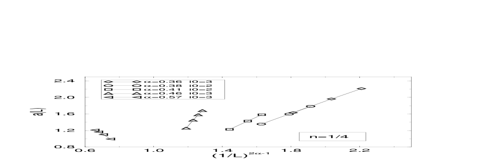
FIG. 6.: Slope $a(L)$ plotted as a function of $L^{1-2\alpha}$ for $n=1/4$ and various interactions ($i_{0}=3$) and for clusters of lengths $L=8$, $12$, $16$ and $20$. Case $\alpha<1$.

The numerical results for $a(L)$ are shown in Fig. 6 and Fig. 7 for various models and are in perfect agreement with the prediction from linear response theory. One can notice that different models (i.e with different ranges $i_{0}$) with almost the same value of $\alpha$ give very similar results. This strongly confirms that only $\alpha$ determines the scaling law. As seen in Fig. 6, for $\alpha<1/2$ the slope $a(L)$ diverges with increasing system sizes. One might thus expect $\delta n(k_{F})$ to vary more rapidly than $t_{\perp}$ and linear response to be no longer valid. The Taylor expansion (19) then breaks down in the thermodynamic limit in this case. On the other hand, for $\alpha>1/2$, $a(L)$ goes to a finite limit when $L\rightarrow\infty$. It is interesting to notice that as one gets close to the cross-over value $\alpha=1$ the fits in terms of a single power law become less accurate since both terms of order $1/L$ and $L^{1-2\alpha}$ compete with each other.

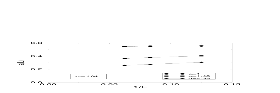
FIG. 7.: Slope $a(L)$ plotted as a function of $1/L$ for $n=1/4$ and various interactions and for clusters of lengths $L=8$, $12$, and $16$. Case $\alpha>1$.

The fact that $a(L)$ remains finite for increasing $L$ (which happens when $\alpha>1/2$) is not sufficient to guaranty the validity of the Taylor expansion. To see this we have investigated the size dependence of the coefficient $b(L)$ of the first non-linear correction.

The numerical estimations of $b(L)$ show unambiguously that $b(L)$ dangerously increases with $L$ at least for $\alpha\lesssim 1$. Moreover $b(L)$ follows very closely a power law behavior $b(L)\sim L^{\gamma}+\hbox{const.}$. The values of the exponents $\gamma$ obtained by a fit of the numerical data are shown in Fig. 8 and are compared to analytic predictions based on a diagrammatic analysis [23]. For $\alpha$ smaller than a certain value, for which the single-particle hopping is more relevant than the two-particle one, the previous RPA treatment (see Sec. III, and also the diagrammatic analysis) suggests that $\gamma=3-4\alpha$. In fact, one can show that at a given order $n$ in the expansion in $t_{\perp}$ the coefficients of the $t_{\perp}^{n}$ term scale like $L^{n(1-\alpha)-\alpha}$ [23]. However, when two-particle interchain hopping becomes dominant, i.e. for $\alpha>\alpha_{2p}$ ($\alpha_{2p}=\sqrt{2}-1\sim 0.41$), there is a cross-over to a different regime. Taking into account the divergence at short distances of some diagrams for the self energy one obtains $\gamma=3-2K-2\alpha$ [9, 23]. Fig. 8 shows indeed an excellent agreement between these predictions and the numerical data. Moreover, it is clear that the results do not depend on the details of the model (e.g. the range $i_{0}$) but only on the value of $\alpha$ characterizing the low-energy behavior. As an additional check, we also show in Figs. 9 and 10 the excellent fits of the numerical data with the expected $L^{\gamma}$ laws in the two regimes.

FIG. 8.: Numerical estimations of $\gamma$ (obtained from a fit) plotted versus $\alpha$. Models of range $i_{0}=3$ ($\bullet$) and $i_{0}=2$ ($\square$) are considered. The analytic predictions (see text) $\gamma=3-4\alpha$ for $\alpha\lesssim\alpha_{2p}$ and $\gamma=3-2\alpha-2K$ for $\alpha\gtrsim\alpha_{2p}$ are shown for comparison as full lines.

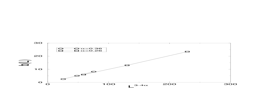
FIG. 9.: Coefficient $b(L)$ ($L=8$, $12$, $16$ and $20$) plotted vs $L^{3-4\alpha}$ in the regime $\alpha<\alpha_{2p}$. The values of $\alpha$ are shown in the plot.

This preliminary analysis shows that there exists a cross-over to a non-linear regime at large system sizes (or, equivalently, small temperatures). The cross-over takes place when the two terms in $\delta n(k_{F})$ become of the same order of magnitude e.g. when $t_{\perp}\gtrsim L^{-(1-\alpha)}$ in the regime $\alpha<\alpha_{2p}$. In the range $1/2<\alpha<1$, even though $a(L)$ has a finite thermodynamic limit, this also happens due to the contribution from higher-order diagrams. This again signals the instability of the Taylor expansion.

FIG. 10.: Coefficient $b(L)$ ($L=8$, $12$, $16$ and $20$) plotted vs $L^{3-2K-2\alpha}$ in the regime $\alpha>\alpha_{2p}$. The values of $\alpha$ are shown in the plot.

The failure of the linear response is signaled in Ref. [24] by the divergence of the linear term at $k=k_{F}$, whenever $\alpha<1/2$. This failure occurs, as expected, only at the interesting point $k=k_{F}$. However, even if the coefficient $a(L)$ of the linear term has a finite limit, one cannot exclude that higher-order terms might become relevant. We have indeed shown numerically that this is the case for the $t_{\perp}^{3}$ term. Actually, due to the relevance of $t_{\perp}$, higher powers of $t_{\perp}$ carry even more divergent terms in the $L\to\infty$ limit. This problem can be also translated into the fact that the $t_{\perp}\rightarrow 0$ and $L\rightarrow\infty$ limits do not commute. By considering the linear behavior, we first take the $t_{\perp}\rightarrow 0$ limit and we study the size dependence of this regime. But, since we are interested in the infinite-volume case, we should consider the opposite limit, in which $L$ is taken to infinity first, i.e. we shall study $\lim_{t_{\perp}\rightarrow 0}\{\lim_{L\rightarrow\infty}\delta n(k_{F})\}$. To perform this, we can gain some insights from the previous study. Indeed, we have obtained the following small-$t_{\perp}$ behavior

$$\delta n(k_{F})\sim(a_{0}+a_{1}L^{1-2\alpha})t_{\perp}-(b_{0}+b_{1}L^{\gamma})t_{\perp}^{3}\ ,$$ (20)

where the $a_{i}$ and $b_{i}$ are $L$-independent constants. Although, in principle, $a_{0}$ and $b_{0}$ could be neglected when $L\gg 1$ and $\alpha<1/2$, in practice, for the sizes $L$ we have studied and when $\alpha$ gets close to $1/2$, it is important to consider the $a_{0}$ term in the following analysis. Let us first focus on the $\alpha<\alpha_{2p}$ regime. Since for $\alpha<\alpha_{2p}$ the dominating term at each finite order $n$ of the Taylor sum is proportional to $t_{\perp}^{n}L^{n(1-\alpha)-\alpha}$, one can group these elements in terms of a scaling function $G_{\alpha}[y]$ of a single variable $y=t_{\perp}L^{1-\alpha}$, obtaining for the Taylor sum a form $G_{\alpha}[y]\ L^{-\alpha}$. Further requiring that the Taylor sum has a finite value in the $L\to\infty$ limit, one can rewrite $G_{\alpha}[y]\ L^{-\alpha}=\tilde{G}_{\alpha}[y]\ y^{\alpha/(1-\alpha)}\ L^{-\alpha}=t_{\perp}^{\alpha/(1-\alpha)}\ \tilde{G}_{\alpha}[y]$, or, equivalently

$$\delta n(k_{F})=a_{0}\ t_{\perp}+t_{\perp}^{\alpha/(1-\alpha)}\ F_{\alpha}(Lt_{\perp}^{1/(1-\alpha)})\ ,$$ (21)

where the $\alpha$-dependent function $F_{\alpha}(x)=G_{\alpha}[x^{1-\alpha}]$ (cf. Ref. [23]) should go to a constant in the $x\to\infty$ limit, and we have restored the linear term that becomes important for $\alpha$ close to or larger than $1/2$. So far, we have proven numerically this scaling form in the regime where the argument $x$ of $F_{\alpha}(x)$ is small, i.e. $t_{\perp}\ll L^{-(1-\alpha)}$. Indeed, using $\gamma=3-4\alpha$, it is easy to rewrite Eq. (20) into the scaling form Eq. (21). If the resummation of the Taylor sum as explained above is justified, the scaling form (21) is not restricted to the range $x\ll 1$ but extends to all values of $x$, in particular to the case $x\rightarrow\infty$ which corresponds to the thermodynamic limit $L\rightarrow\infty$ at fixed $t_{\perp}$. In this case, as explained above, one expects the function $F_{\alpha}$ to have a finite limit, $\lim_{x\rightarrow\infty}F_{\alpha}(x)=c_{\alpha}$, since $\delta n(k_{F})$ is finite in the infinite-volume limit. Therefore, formula (21) leads naturally to $\delta n(k_{F})=c_{\alpha}\,t_{\perp}^{\alpha/(1-\alpha)}$. Note that for $\alpha<1/2$ the contribution of the $a_{0}t_{\perp}$ term can be neglected for small $t_{\perp}$ since the exponent $\alpha/(1-\alpha)$ is smaller than unity.

To investigate numerically the validity of the scaling relation (21) for all values of the argument of $F_{\alpha}$ we proceed as follows; from the numerical data $\delta n(k_{F})$ and the previous estimations of the constant $a_{0}$ (which depends on $\alpha$) we construct the quantity

$$F_{\alpha}^{\prime}(L,t_{\perp})=(\delta n(k_{F})-a_{0}t_{\perp})/t_{\perp}^{\alpha/(1-\alpha)}$$ (22)

which, a priori is a function of $L$ and $t_{\perp}$ independently.

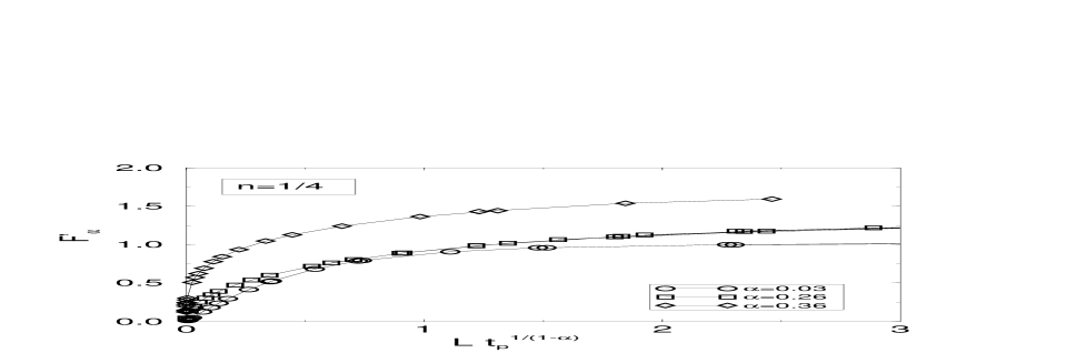
FIG. 11.: $F_{\alpha}^{\prime}(L,t_{\perp})$ for various values of $t_{\perp}$ and for lengths $L=8$, $12$, $16$ and $20$ as a function of a unique variable $Lt_{\perp}^{1/(1-\alpha)}$.

In Fig. 11 $F_{\alpha}^{\prime}$ is plotted as a function of the combined variable $Lt_{\perp}^{1/(1-\alpha)}$. As can be seen on the plot, it is striking that, for $\alpha<\alpha_{2p}$, all the data sets lie on a single curve. The scaling hypothesis is then verified to a high accuracy. This unique curve then defines the scaling function $F_{\alpha}(x)$ where $x=Lt_{\perp}^{1/(1-\alpha)}$. From Fig. 11 it is also clear that, when $x\rightarrow\infty$, the function $F_{\alpha}(x)$ saturates to a finite value which, according to the previous discussion, implies the asymptotic law

$$\delta n(k_{F})\propto t_{\perp}^{\alpha/(1-\alpha)}\ ,$$ (23)

in the thermodynamic limit.

FIG. 12.: $\delta n(k_{F})$ vs $t_{\perp}$ for various interactions calculated on $2\times 8$ ($\circ$), $2\times 12$ ($\square$) and $2\times 16$ ($\lozenge$) ladders. The thermodynamic limit, for $\alpha<1/2$, $\delta n=c_{\alpha}\,t_{\perp}^{\alpha/(1-\alpha)}+a_{0}t_{\perp}$ (where $c_{\alpha}$ is estimated from Fig. 11 and the linear $t_{\perp}$ term is subdominant at small $t_{\perp}$) is also shown as dashed lines. $V=1$, $2$, $3$ and $5$ correspond to $\alpha=0.10$, $0.26$, $0.46$ and $1.00$ respectively. For $V=5$, the dashed line corresponds to a linear term only.

For comparison, we have plotted in Fig. 12 the raw data and the expected $L\to\infty$ behaviors according to (21) for the quantity $\delta n(k_{F})$ as a function of $t_{\perp}$. It is very clear from this plot that the finite-size effects are particularly strong when $t_{\perp}$ is small. This result can be qualitatively understood since, as we explained above, the thermodynamic limit is obtained when $Lt_{\perp}^{1/(1-\alpha)}\rightarrow\infty$. A typical length scale $L_{\text{typ}}(t_{\perp})$ is defined from the scaling behavior and $L_{\text{typ}}$ increases rapidly with decreasing $t_{\perp}$ as $t_{\perp}^{-1/(1-\alpha)}$.

Our scaling results for $\alpha<\alpha_{2p}$ are in excellent agreement with the predictions based on the approximate (RPA) Green’s function Eq. (8), as long as exponents are concerned. This agreement is expected to persist at least as long as the coherent two-particle interchain hopping does not play an important role, i.e. up to the value of $\alpha_{2p}$. The approximation first made by Wen that consists in neglecting the vertex corrections in the computation of the Green’s function turns out not to be dramatic as proven here numerically, due to the fact that higher-order corrections build up in an homogeneous way.

As stated in Sec. IV, RG calculations [8, 9] predict a cross-over from a one-particle regime to a two-particle regime around $\alpha=\alpha_{2p}\sim 0.41$. Physically, in this regime particle-hole hopping dominates with respect to single-particle hopping. This cross-over is also signaled by the change in behavior of the exponent $\gamma$ governing the size dependence of $b(L)$ as seen in Fig. 8. In fact, in the regime $\alpha>\alpha_{2p}$, the diagrammatic expansion of the self-energy generates nonhomogeneous contributions at higher orders in $t_{\perp}$ so that a re-summation in a simple scaling form similar to (21) is quite difficult. By taking into account the leading diagrams contributing to the self-energy, it has been shown that this crossover changes the functional form of the exponent of the behavior of $\delta n(k_{F})$ as a function of $t_{\perp}$ also in the thermodynamic limit. For $L\gg 1$ and $t_{\perp}\ll t$ one can argue the scaling behavior

$$\delta n(k_{F})=t_{\perp}^{\alpha/(1-K)}F_{K}(t_{\perp}^{1/(1-K)}L)+a_{0}t_{\perp}$$ (24)

whose derivation is however not straightforward due to the contribution of different inhomogeneous diagrams [23]. In this equation, $K$ can be expressed as a function of $\alpha$ by inverting the equation $\alpha=\frac{1}{2}(K+1/K-2)$. In particular, $K$ becomes smaller than $\alpha$ for $\alpha>\alpha_{2p}$, therefore the new exponent ${\alpha/(1-K)}$ is reduced with respect to ${\alpha/(1-\alpha)}$ and dominates the small-$t_{\perp}$ regime. One important consequence of this different scaling behavior is that the anomalous contribution $t_{\perp}^{\alpha/(1-K)}$ dominates with respect to the linear contribution $a_{0}t_{\perp}$ in a larger parameter range, i. e. the behavior of $\delta n(k_{F})$ is sublinear up to $\alpha=2/3$ (and not only to $\alpha=1/2$ as obtained within the RPA approximation). This is interesting since linear response theory, while on the one hand predicting its own failure at $\alpha<1/2$, due to the divergence of the coefficient $a(L)=a_{0}+a_{1}L^{1-2\alpha}$ in Eqs. (19-20), on the other hand would lead to a regular linear behavior for $\alpha>1/2$, in contrast with the result of Eq. (24).

Eq. (24) has been obtained by cutting the expansion of the self energy at a given finite order in $t_{\perp}$ [23]. Due to the inhomogeneity of the diagrams, this procedure might not produce the correct result, if the Taylor series sums up in some unexpected way. It is thus of great importance to verify numerically whether there is a deviation at all from the scaling behavior Eq. (21) for $\alpha>\alpha_{2p}$ and, if this is the case, to verify whether the scaling law Eq. (24), and thus the $L\rightarrow\infty$ behavior $\delta n(k_{F})=t_{\perp}^{\alpha/(1-K)}$ are verified. Of course, the deviation of the behavior of the exponent $\gamma$ from the dashed line shown in Fig. 8 already tells us that something is changing for $\alpha>\alpha_{2p}$. However, this figure does not tell us anything about the thermodynamic limit.

The presence of several inhomogeneous contributions for $\alpha>\alpha_{2p}$ complicates substantially the numerical analysis too. For values of $\alpha$ not too far from $\alpha_{2p}$ (in our case for $\alpha\approx 0.57$) it is difficult to distinguish between the two scaling behaviors Eqs. (21) and (24), due to the small difference between the exponents $\alpha/(1-K)$ and $\alpha/(1-\alpha)$. Moreover, we shall show that the effects of the two-particle contributions start to be dominating only at large $L$, thus forcing us to a careful finite-size analysis. In Fig. (13), we plot the results of the scaling for a larger value of $\alpha$, namely $\alpha=0.7$. In curves (a) and (b) we proceed in the usual way by plotting the quantity $F_{\eta}^{\prime}=(\delta n(k_{F})-a0\ t_{\perp})/t_{\perp}^{\alpha/(1-\eta)}$ as a function of $x_{\eta}=t_{\perp}^{1/(1-\eta)}L$, where $\eta$ takes the two values $\eta=\alpha$ in (a) and $\eta=K$ in (b), corresponding to the two laws Eqs. (21) and (24), respectively. In both cases, the scaling ansatz seems rather poor, thus showing at least that something has changed for large $\alpha$ since the scaling Eq. (21) no longer works (Fig. 13 curve (a)). In order to improve our accuracy, we further subtract the whole linear contribution from $\delta n(k_{F})$ and plot in (c) the quantity $F_{\eta,L}^{\prime}=(\delta n(k_{F})-a(L)\ t_{\perp})/t_{\perp}^{\alpha/(1-\eta)}$ as a function of $x_{\eta}=t_{\perp}^{1/(1-\eta)}L$ with $\eta=K$. The subtraction of the $L$-dependent term is harmless in the thermodynamic limit, since $a(L\rightarrow\infty)\rightarrow a_{0}$ for $\alpha>1/2$. However, this subtraction allows us to eliminate competing terms that would make the numerical analysis difficult. This curve plotted as (c) in Fig. (13) shows that the fit is indeed rather good. This shows numerically that for large $L$ the scaling Eq. (24) is the appropriate one.

FIG. 13.: $F_{\eta}^{\prime}(L,t_{\perp})$ for $\eta=\alpha$ (a) and for $\eta=K$ (b) and $F_{\eta,L}^{\prime}(L,t_{\perp})$ for $\eta=K$ (c) for various values of $t_{\perp}$ and for lengths $L=8$, $12$, $16$ plotted as a function of the variable $x_{\eta}=t_{\perp}^{1/(1-\eta)}\,L$ (cf. text). The interaction $V=4$, $i_{0}=3$ corresponds to $\alpha=0.7$.

The only flaw of curve (c) in this figure is that it is not clear whether $F_{\eta}(x)$ goes to a constant in the thermodynamic ($x\rightarrow\infty$) limit. This should however be expected on physical grounds. The reason why this curve does not yet saturates is that the system sizes considered are still too small to reach the thermodynamic limit in the two-particle regime. That is also the reason for which it was important to subtract the whole ($L$-dependent) linear contribution to $\delta n(k_{F})$.

VI Conclusions

In this paper, ground-state correlation functions of strongly-correlated coupled chains were investigated by numerical exact-diagonalization techniques. First of all, the low-energy LL properties of the $1D$ correlated chains were entirely characterized by the Luttinger Liquid correlation exponent $\alpha$. The values of $\alpha$ were calculated from a finite-size scaling analysis for various strengths and ranges of the electron-electron interaction. The correct $\alpha$-dependence of the scaling behaviors of known $1D$ correlation functions were recovered. In a second step, the expectation value of the single-particle hopping operator between two coupled chains at $k=k_{F}$ was investigated by similar ED methods supplemented by finite-size scaling analysis. The Taylor expansion of the expectation value of the single-particle hopping operator in powers of $t_{\perp}$ was shown to become unstable in the thermodynamic limit in agreement with the theoretical prediction that the single-particle hopping is relevant. A change of behavior of the size scaling of the coefficient of the $t_{\perp}^{3}$ term for $\alpha$ greater than a critical value $\alpha_{2p}$ is attributed to the coherent transverse two-particle hopping becoming the dominant perturbation. In addition, in the regime $\alpha<\alpha_{2p}$ where transverse two-particle hopping is less relevant, the finite-size effects can be described in terms of a universal scaling function. In the thermodynamic limit, it is found that the expectation value of the single-particle interchain hopping operator at momentum $k_{F}$ behaves as $t_{\perp}^{\alpha/(1-\alpha)}$ in agreement with an RPA-like treatment of the interchain coupling. In contrast, in the $\alpha>\alpha_{2p}$ regime a crossover to a $t_{\perp}^{\alpha/(1-K)}$ law is observed (dominated by a linear contribution when $\alpha>2/3$), signaling the dominance of two-particle hopping processes.

Whether the coupled-chain system behaves as an ordinary Fermi Liquid is still not clear yet. The energy splitting between bonding and antibonding states (which should be related to the warping of the Fermi surface) calculated numerically in Ref. [14] varies as $t_{\perp}^{1/(1-\alpha)}$ as suggested by analytic treatments [23]. However, for large enough $\alpha$ this behavior might occur only above a critical value of $t_{\perp}$ (see Ref. [14]). Let us also mention that transport properties in the direction perpendicular to the chains should follow power laws in $t_{\perp}$. Numerical results for the Drude weight [14] are indeed compatible with $t_{\perp}^{\nu}$, $\nu>2$.

We acknowledge many fruitful discussions with M. G. Zacher and W. Hanke. Laboratoire de Physique Quantique, Toulouse is Unité Mixte de Recherche CNRS No 5626. We thank IDRIS (Orsay) for allocation of CPU time on the C94 and C98 CRAY supercomputers. E. A. gratefully acknowledges research support by the EC-TMR program ERBFMBICT950048 and thanks the Laboratoire de Physique Quantique de Toulouse for its hospitality during which part of this work has been done.

REFERENCES

- [1] L. P. Gor’kov and I. E. Dzyaloshinskii, Sov. Phys. JETP 40, 198 (1974); H. J. Schulz, Int. J. Mod. Phys. 5, 57 (1991); C. Castellani, C. D. Castro, and W. Metzner, Phys. Rev. Lett. 72, 316 (1994).
- [2] P. W. Anderson, Phys. Rev. Lett. 67, 3844 (1991); P. W. Anderson, Science 256, 1526 (1992).
- [3] S. P. Strong, D. G. Clarke, and P. W. Anderson, Phys. Rev. Lett. 73, 1007 (1994).
- [4] C. Jacobsen, D. B. Tanner and K. Bechgaard, Phys. Rev. Lett. 46, 1142 (1981); J. R. Cooper et al., Phys. Rev. B 33, 6810 (1986); J. Moser, M. Gabay, P. Auban-Senzier, D. Jérome, K. Bechgaard, J. M. Fabre, preprint (1997).
- [5] G. M. Danner and P. M. Chaikin, Phys. Rev. Lett. 75, 4690 (1995).
- [6] F. D. M. Haldane, J. Phys. C 14, 2585 (1981).
- [7] X. G. Wen, Phys. Rev. B 42, 6623 (1990).
- [8] C. Bourbonnais and L. G. Caron, Int. J. Mod. Phys. B 5, 1033 (1991).
- [9] S. A. Brazovskii and V. M. Yakovenko, Sov. Phys. JETP 62, 1340 (1985); V. M. Yakovenko, Pis’ma Zh. Exp. Theor. Fiz. 56, 523 (1992) [JETP Lett. 56, 510 (1992)]; A. A. Nersesyan, A. Luther and F. V. Kusmartsev, Phys. Lett. A 176, 363 (1993).
- [10] D. G. Clarke, S. P. Strong, and P. W. Anderson, Phys. Rev. Lett. 72, 3218 (1994).
- [11] F. Mila and D. Poilblanc, Phys. Rev. Lett. 76, 287 (1996); see also D. G. Clarke and S. P. Strong, Phys. Rev. Lett. 78, 563 (1997); F. Mila and D. Poilblanc, Phys. Rev. Lett. 78, 564 (1997).
- [12] D. Poilblanc, H. Endres, F. Mila, M. Zacher, S. Capponi and W. Hanke, Phys. Rev. B 54, 10261 (1996).
- [13] For technical details see e.g. D. Poilblanc in “Numerical methods for strongly correlated systems”, Frontiers in Physics, Ed. D. J. Scalapino, Addison-Wesley, Redwood City California (1997).
- [14] S. Capponi, D. Poilblanc and F. Mila, Phys. Rev.54, 17547 (1996).
- [15] H. J. Schulz, “Correlated Electron Systems”, p. 199, ed. V. J. Emery (World scientific, Singapore, 1993); H. J. Schulz, “Strongly Correlated Electronic Materials: The Los Alamos Symposium – 1993”, p. 187, ed. K. S. Bedell, Z. Wang, D. E. Meltzer, A. V. Balatsky, E. Abrahams (Addison-Wesley, Reading, Massachussets, 1994).
- [16] J. Voit, Rep. Prog. Phys. 58, 977 (1995) and references therein.
- [17] H. W. J. Blöte, J. L. Cardy and M. P. Nightingale, Phys. Rev. Lett. 56, 742 (1986); I. Affleck, ibid. p. 746.
- [18] See D. Boies, C. Bourbonnais, and A.-M.S. Tremblay, Phys. Rev. Lett. 74, 968 (1995) and references therein.
- [19] A. M. Tsvelik, cond-mat/9607209 preprint.
- [20] C. Bourbonnais, Ph. D. thesis, Université de Sherbrooke, 1985 (unpublished).
- [21] J. Voit, Phys. Rev. B 47, 6740 (1993).
- [22] J. Voit, J. Phys: Cond. Mat. 5, 8305 (1993).
- [23] E. Arrigoni, preprint (1997).
- [24] C. Castellani, C. di Castro and W. Metzner, Phys. Rev. Lett. 69, 1703 (1992).
- [25] P. Kopietz, V. Meden and K. Schönhammer, Phys. Rev. Lett. 74, 2997 (1995); P. Kopietz, V. Meden and K. Schönhammer, cond-mat/9701023 (1997); See also A. Houghton and J. B. Marston, Phys. Rev. B 48, 7790 (1993).
- [26] For a presentation of these models, see e.g. N. Shannon, Y. Li and N. d’Ambrumenil, cond-mat/9611071; L. Bartosch and P. Kopietz, Phys. Rev. B 55, 15360 (1997).
- [27] H. J. Schulz, J. Phys. C 16, 6769 (1983).
- [28] Similar behaviors were also found for the energy splitting between bonding and antibonding states in coupled chains of spinful (Ref. [12]) or spinless particles (Ref. [14]).