Quasi-linear magnetoresistance in an almost two-dimensional band structure

Abstract

We present a theoretical study of the orbital magnetoresistance in a unixial anisotropic metal within the relaxation-time approximation. The appearance of a new dimensionless scale, $\delta=4t_{\perp}/\epsilon_{F}$, allows the possibility of a new region at intermediate fields where the magnetoresistance is linear in applied magnetic field for currents flowing along the unixial direction. (Here, $t_{\perp}$ characterizes the bandwidth along the unixial direction.) In the limit of large anisotropy (small $\delta$), corresponding to a quasi-two-dimensional metal made up of weakly coupled layers, we obtain an analytic expression for the magnetoresistance valid for all magnetic fields. We test our analytic results numerically and we compare our expressions with the $c$-axis magnetoresistance of $\rm Sr_{2}RuO_{4}$.

I Introduction

A growing number of compounds have been synthesized whose crystal structure consists of weakly coupled metallic layers. Foremost among these are the cuprate metals where the two-dimensional nature electronic structure has provoked much speculation about the nature of the resulting metallic state. The issue of whether in-plane excitations can move coherently between copper oxide planes remains contentious strong . Several other metallic compounds with a layered structure—for example organic compounds based on the bis-ethylenedithiotetrathiafulvalene molecule and other metallic oxides such as $\rm Sr_{2}RuO_{4}$—do possess a Fermi surface which is shaped like a slightly warped cylinder mackenzie . In this paper we study magnetotransport in a quasi-two-dimensional (2D) metal in order to provide a benchmark against which more exotic types of behavior can be compared. Specifically we study out-of-plane transport using the relaxation-time approximation in the presence of an in-plane magnetic field. Our main result is that there is a “Kapitza” region kapitza where the transverse magnetoresistance $\Delta\rho_{c}/\rho_{c}$ is proportional to the applied magnetic field. We justify this with an analytic expression for the magnetoresistance in the quasi-two-dimensional limit which is valid for arbitrary magnetic fields. We also obtain an expression for the magnetoresistance with any degree of unixial anisotropy that can be evaluated numerically.

The study of magnetotransport within the Boltzmann formalism is long established and is well described in a number of classic textsabrikosov ; pippard . Interpreting magnetoresistance measurements is complicated by the fact that the magnetoresistance is identically zero for an isotropic metal. The amount of anisotropy determines the measured magnetoresistance, which is therefore rather sensitive to the detailed properties of the material. Analytic results are usually limited to the very weak or very high-magnetic-field regimes. At low fields the Zener-Jones expansion yields a magnetoresistance quadratic in the magnetic field with a coefficient depending on the variation of the mean-free-path around the Fermi surface. At high fields the magnetoresistance saturates when current flow is along closed Fermi-surface directions or maintains a quadratic field dependence for currents along open Fermi-surface directions (see page 118 of Ref. abrikosov, ). To our knowledge, there have been no analytic expressions for the magnetoresistance of a realistic bandstructure which interpolate between these known limits.

In this paper we present a calculation which, while respecting the high- and low-field results mentioned above, also applies at intermediate fields where we find a linear magnetoresistance. We have obtained an analytic expression for the magnetoresistance, valid in the limit of strong anisotropy, which we believe to be the first straightforward example of a magnetoresistance formula valid for all magnetic fields. This result should prove useful in characterizing the properties of quasi-two-dimensional metals using transport measurements. The paper is organized as follows. We first present a simple calculation of the magnetoconductance that illustrates how having a warped cylindrical Fermi surface can give rise to a linear magnetoresistance. We then present a more formal solution of the Boltzmann equation and derive the conductivity tensor for arbitrary levels of anisotropy. Our analytic result emerges as a limiting case. Finally we discuss the implications of these results for experiment and compare with known data.

II Simple picture

We consider a metal with the following dispersion relation

$$\epsilon(\vec{k})={\hbar^{2}\over 2m_{\circ}}\left(k_{x}^{2}+k_{y}^{2}\right)-2t_{\perp}\cos\left(k_{z}c\right)+2t_{\perp}\;.$$ (1)

We have adopted the customary notation that directions in reciprocal space are labeled $x$, $y$, and $z$ while the corresponding real space lattice is defined by the $a$, $b$ and $c$ directions. It describes free particles in the $ab$ plane coupled by a perpendicular transfer integral, $t_{\perp}$ in the $c$ direction to adjacent planes. The magnitude of $c$ gives the spacing between planes that can be combined with $t_{\perp}$ to form an effective mass for out-of-plane motion

$$m_{\perp}=\hbar^{2}/2t_{\perp}c^{2}\;.$$ (2)

(This is the $z$-axis band mass in the limit $\epsilon_{F}\ll t_{\perp}$ when the Fermi surface forms a closed spheroid.)

We begin with an approximate derivation of the new regime by considering the magnetoconductance to lowest order in $t_{\perp}$. Chambers’ expression chambers for the components of the conductivity tensor in a magnetic field within the relaxation-time approximation is

$$\sigma_{ij}={e^{2}\over 4\pi^{3}}\oint{dS\over\hbar|\vec{v}|}\int_{0}^{\infty}v_{i}(0)v_{j}(t)e^{-t/\tau}dt\;.$$ (3)

For each area element of the Fermi surface, $dS$, we integrate the velocity $\vec{v}(t)$ measured along a semiclassical quasiparticle orbit. These orbits are defined by the Lorentz equation of motion

$$\hbar{d\vec{k}\over dt}=-e\vec{v}\times\vec{B}\;,$$ (4)

where $\vec{v}=\vec{\nabla}_{k}\epsilon(\vec{k})/\hbar$. In this paper we will be interested in configurations where the magnetic field is parallel to the planes and the current is flowing perpendicular to the planes [see Fig. (1a)].

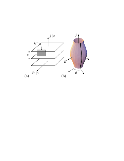
Figure 1: The field geometry and approximate quasiparticle orbits—here shown for $\delta=2/3$. (a) The magnetic field lies in the plane and the current flows out of the plane. The linear magnetoresistance regime occurs when the magnetic flux through a loop defined by the in-plane mean-free-path, $l_{\circ}$, and the plane separation, $c$, becomes of the order of a flux quantum or greater. (b) In the limit of large anisotropy, we can approximate the quasiparticle orbits as lines on the Fermi surface with constant radial angle $\theta$ and constant in-plane velocity $v_{\circ}$. This gives an approximate derivation of the low-field ($B^{2}$) and intermediate-field ($|B|$) regions.

To lowest order in $t_{\perp}$ we can ignore both the $z$-axis dispersion in the equation of motion and the closed orbits. The rate of change of ${\vec{k}}$ then only depends on the angle $\theta$ between the magnetic field and the in-plane Fermi velocity of an electron [see Fig. (1b)]. So we have

$$\hbar{dk_{z}\over dt}=-ev_{\circ}B\sin\theta\;,$$ (5)

where the in-plane Fermi velocity, $v_{\circ}$, is constant here. Hence we see that

$$ck_{z}(t)=ck_{z}(0)+\Omega_{c}t\sin\theta\;.$$ (6)

We can determine how the velocity in the $c$ direction changes as the quasiparticle moves across the Fermi surface by combining the above result with Eq. (1) giving

$$v_{c}(t)={2t_{\perp}c\over\hbar}\sin\left[k_{z}c+\Omega_{c}t\sin\theta\right]\;.$$ (7)

Here we have defined a “cyclotron” frequency

$$\Omega_{c}={ev_{\circ}Bc\over\hbar}\;,$$ (8)

which is the fastest rate at which quasiparticles traverse the Brillouin zone. It turns out that this sets the scale of the crossover from weak ($\Omega_{c}\tau\ll 1$) to intermediate fields ($\Omega_{c}\tau\gtrsim 1$).

Substituting this velocity, $v_{c}(t)$, into the expression for the conductivity Eq. (3), we may integrate over time and $k_{z}$ to give the out-of-plane conductivity expressed as an integral over the orbits, namely,

$$\sigma_{c}(B)={e^{2}t_{\perp}^{2}\tau k_{F}c\over\pi^{2}\hbar^{3}v_{\circ}}\int_{0}^{2\pi}{d\theta\over 1+\Omega_{c}\tau^{2}}\;.$$ (9)

Integrating this is straightforward and yields the following magnetoconductance

$${\Delta\sigma_{c}(B)\over\sigma_{c}(0)}={1\over\sqrt{1+\Omega^{2}_{c}\tau^{2}}}\;.$$ (10)

At low fields ($\Omega_{c}\tau\ll 1$) this gives the usual quadratic field dependence as obtained by the Zener-Jones expansion. However in the intermediate field regime $(\Omega_{c}\tau\gtrsim 1)$ the magnetoconductivity falls off as $1/B$. This is the essential result of this paper. It arises because there is a range of cyclotron frequencies for traversing the Brillouin zone. Note too that the magnetoconductance becomes universal, independent of the degree of anisotropy and depending only on the in-plane properties. We can emphasize this by writing the cross-over condition in terms of the magnetic length $l_{B}^{2}=\hbar/eB$, namely $\Omega_{c}\tau=1$ corresponds to

$${l_{\circ}c\over l_{B}^{2}}=1\;.$$ (11)

So the linear region is reached when approximately one flux quantum threads an area formed by the in-plane mean-free-path ($l_{\circ}=v_{\circ}\tau$) and the interplanar spacing. For a typical layered oxide ($c\sim 12$Å) one can expect to see this regime at 10 Tesla when the in-plane mean free path reaches around 500 Å. As discussed later, experiments hussey_1997 on $\rm Sr_{2}RuO_{4}$ provide evidence for the validity of this expression.

However, this cannot be the complete story since very general arguments show that $\sigma_{c}$ must go as $1/B^{2}$ at high fieldsabrikosov . Since the conductivity is the sum of the conductivities from all orbits, the high-field form cannot be recovered simply by including the contribution of the closed orbits: a $1/B^{2}$ contribution from closed orbits will never dominate the $1/B$ from open orbits. The correct high field result emerges when we consider higher-order effects in $t_{\perp}$ for both the open and closed orbits in the exact solution of section III. We will see that the high field $1/B^{2}$ regime occurs when $\Omega_{c}\tau\gg\sqrt{\epsilon_{F}/t_{\perp}}$.

A further reason for a more detailed treatment is that the magnetoresistance is identically zero for an ellipsoidal Fermi surface with a constant $\tau$. This is because of a cancellation between the Hall and magnetoconductance. We therefore would like to verify that there is no such cancellation here. We will do this through an exact solution of the Boltzmann equation in which we compute all components of the conductivity tensor and hence the magnetoresistance.

III Solving the Boltzmann Equation

Our treatment will follow closely that of Abrikosov abrikosov . In the previous section we only treated the quasiparticle orbits approximately. Since the Lorentz force in Eq. (4) acts perpendicular to the electron motion, energy is conserved and the electron is constrained to move along a constant energy line with fixed momentum in the $\vec{B}$ direction. Here we take $B$ to be parallel to $a$. For finite $t_{\perp}$, $\theta$ is no longer constant along the orbits and there are some closed orbits as illustrated in Fig. (2a).

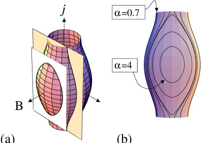
Figure 2: The exact orbits over the Fermi surface with $\delta=2/3$. (a) The quasiparticle moves along lines defined by the intersection of the Fermi surface and planes perpendicular to the field direction. These orbits can be either open or closed and are described by Jacobi elliptic functions. (b) We can label these orbits by a parameter $\alpha$, the parameter of the Jacobi elliptic function. Here we illustrate orbits where $\alpha=0.7,0.9,0.99,1.01,1.5$ and $4$. For $\delta\leq\alpha\leq 1$ the orbits are open. For $1\leq\alpha<\infty$ the orbits are closed.

Quasiparticles at the Fermi surface determine the transport properties and we may identify two regions depending on the degree of anisotropy. We introduce a parameter which is a measure of this anisotropy

$$\delta={4t_{\perp}\over\epsilon_{F}}\;.$$ (12)

If $\delta>1$, the Fermi surface is closed and the trajectory of all quasiparticles in momentum (and real) space follows closed loops. While the system may have an anisotropic effective mass, the qualitative features of transport will not be much modified from a typical three-dimensional metal. If $\delta<1$ then we still have some closed orbits but there are now some trajectories that extend across the Brillouin zone in the $c$ direction [see Fig. (2a)]. Only these orbits have been treated in section II (and then only approximately). We now aim for a more complete analysis.

To consider the conductivity tensor we must solve the Boltzmann equation. Rather than use the momentum components $k_{x}$, $k_{y}$ and $k_{z}$, in the presence of a magnetic field it is more convenient to work in terms of a new coordinate system $k_{x},\epsilon,$ and $t$. Here $t$ is the time taken to move along the momentum orbits defined by the equation of motion, Eq. (4). The advantage of this coordinate system is that the magnetic field is included implicitly and does not appear in the Boltzmann equation. Within the relaxation-time approximation, one may write the Boltzmann equation as abrikosov ,

$${\partial\psi\over\partial t}+{\psi\over\tau}=e\vec{E}\cdot\vec{v}\;,$$ (13)

where the electron distribution function has been written as $f=f^{(0)}-\psi\partial_{\epsilon}f^{(0)}$. This first-order differential equation may be solved straightforwardly.

Substituting into Eq. (4) gives

$$dt = -{m_{\circ}\hbar\over eB}{dk_{z}\over\sqrt{2m_{\circ}\epsilon-\hbar^{2}k_{x}^{2}+4m_{\circ}t_{\perp}\left[\cos\left({k_{z}c}\right)-1\right]}}\;,$$ (14)

$$= -{\sqrt{\alpha}\over\omega_{c}}{c\over 2}{dk_{z}\over\sqrt{1-\alpha\sin^{2}\left({k_{z}c/2}\right)}}\;,$$ (15)

where

$$\alpha={8t_{\perp}m_{\circ}\over 2m_{\circ}\epsilon_{F}-\hbar^{2}k_{x}^{2}}\;.$$ (16)

We have defined a new “cyclotron” frequency cyclotron

$$\omega_{c}={eBc\over\hbar}\sqrt{2t_{\perp}\over m_{\circ}}={eB\over\sqrt{m_{\circ}m_{\perp}}}=\Omega_{c}\sqrt{\delta\over 4}\;,$$ (17)

the fastest rate at which quasiparticles perform closed orbits. This is the natural scale for cyclotron motion perpendicular to the plane. As might be anticipated from a Bohr quantization picture, it also sets the scale for Landau-level quantization and hence the quantum effects which signal the breakdown of quasi-classical transport theory. The variable $\alpha$ labels each cyclotron orbit. It is bounded from below by $\delta$ and we will use it to substitute for $p_{a}$

$$\hbar k_{x}=\sqrt{2m_{\circ}\epsilon-8t_{\perp}m_{\circ}/\alpha}\;.$$ (18)

The orbits are open for $\delta<\alpha<1$ and closed for $1<\alpha<\infty$.

It is very unusual that Eq. (15) is both integrable and its solution is invertible so that a closed form expression for the orbits may be found. The solution can be written in terms of the Jacobian elliptic functions

$$k_{z}(t) = -{2\over c}{\rm JacobiAmplitude}\left[{\omega_{c}t\over\sqrt{\alpha}},\alpha\right],$$ (19)

$$v_{c}(t) = -{2\hbar\over cm_{\perp}}{\rm JacobiCN}\left[{\omega_{c}t\over\sqrt{\alpha}},\alpha\right]{\rm JacobiSN}\left[{\omega_{c}t\over\sqrt{\alpha}},\alpha\right],$$

$$v_{b}(t) = {2\hbar\over c\sqrt{\alpha m_{\perp}m_{\circ}}}{\rm JacobiDN}\left[{\omega_{c}t\over\sqrt{\alpha}},\alpha\right].$$ (21)

These equations exactly describe the quasiparticle’s motion over the Fermi surface defined by Eq. (1) in the presence of a magnetic field along the $a$ direction. We have adopted the notation of Mathematica wolfram and Abromowitz and Stegun AS in using the parameter $\alpha$ rather than the modulus, $k=\sqrt{\alpha}$, to define these functions.

These periodic functions play the role of the trigonometric functions that appear in the solution of the spherical problem. To make this more explicit, we can map the elliptic functions when the parameter $\alpha$ is greater than one (describing closed orbits) to those with a parameter $\beta=1/\alpha$ less than one AS . We may then write

$$v_{c}(t) = -{2\sqrt{\beta}\hbar\over cm_{\perp}}{\rm JacobiDN}[\omega_{c}t,\beta]{\rm JacobiSN}[\omega_{c}t,\beta]\;,$$ (23)

$$\lim_{\beta\rightarrow 0}-{2\hbar\over c}{\sqrt{\beta}\over m_{\perp}}\sin(\omega_{c}t)\;,$$

$$v_{b}(t) = {2\hbar\over c}\sqrt{\beta\over m_{\perp}m_{||}}{\rm JacobiCN}[\omega_{c}t,\beta]\;,$$ (24)

$$= \lim_{\beta\rightarrow 0}{2\hbar\over c}\sqrt{\beta\over m_{\perp}m_{\circ}}\cos(\omega_{c}t)\;,$$ (25)

The limiting case of $\beta\rightarrow 0$ describes all of the orbits when the Fermi surface becomes spheroidal ($\delta\rightarrow\infty$).

To compute the conductivities we use the solution of the Boltzmann equation [Eq. (13)] and compute the current. This gives the Chambers’ formula [Eq. (3)] which may be written as (see Ref. [abrikosov, ])

$$j_{\alpha}={2e^{2}B\over\left(2\pi\hbar\right)^{3}}\int_{-p_{a}^{0}}^{p_{a}^{0}}\!\!\!\!\!\!dp_{a}\int_{0}^{T(p_{a})}\!\!\!\!\!\!\!\!dt\int_{-\infty}^{t}\!\!\!\!\!\!\!dt^{\prime}v_{\alpha}(t)v_{\beta}(t^{\prime})E_{\beta}e^{(t^{\prime}-t)/\tau}\;.$$ (26)

This triple integral can be drastically simplified when we recall that the orbits are all periodic and so have a well-defined Fourier series. The Fourier series for the Jacobian elliptic functions are all tabulated GR . This allows one to do the integral over $t^{\prime}$ and, using the orthogonality of the components of the Fourier series, one can also do the integral over $t$. The algebra is somewhat tedious but the result is that the conductivity can be expressed as a rapidly convergent sum followed by a single integral over $p_{a}$.

We will use the definition of the tensor conductivity $j_{\alpha}=\sigma_{\alpha\beta}E_{\beta}$ with the magnetic field along the $a$ direction. The only nonzero components of the conductivity tensor will be $\sigma_{aa}$, $\sigma_{bb}$, $\sigma_{cc}$ and $\sigma_{bc}=-\sigma_{cb}$. There is no longitudinal magnetoresistance for the dispersion of Eq. (1) so $\sigma_{aa}$ is unaffected by the magnetic field and, by rotational symmetry in the $ab$ plane, will be equal to $\sigma_{bb}$ in the absence of a magnetic field. We can simplify some of the expressions by introducing a number of parameters: a universal conductivity and the effective-mass ratio

$$\sigma_{0}={2e^{2}\tau\over c^{3}m_{\perp}}\;,\quad\quad r={m_{\circ}\over m_{\perp}}\;.$$ (27)

For the exact solution of the conductivity tensor we find the following components

$$\sigma_{aa} = {\sigma_{0}\over\pi^{3}\sqrt{\delta}}\left[4\int_{\min(1,\delta)}^{1}{K(\alpha)\sqrt{\alpha-\delta}\over\alpha^{2}}d\alpha+\int_{0}^{\min(1,\delta^{-1})}K(\beta)\sqrt{1-\beta\delta}d\beta\right]\;,$$ (28)

$$\sigma_{bb} = {\sigma_{0}\sqrt{\delta}\over\pi}\left[\int_{\min(1,\delta)}^{1}{1+8S_{1}(\alpha,\omega_{c}\tau/\sqrt{\alpha})\over K(\alpha)\sqrt{\alpha-\delta}}d\alpha+8\int_{0}^{\min(1,\delta^{-1})}{\tilde{S}_{1}\left(\beta,\omega_{c}\tau\right)\over K(\beta)\sqrt{1-\beta\delta}}d\beta\right]\;,$$ (29)

$$\sigma_{cc} = {2\pi r\sigma_{0}\sqrt{\delta}}\left[4\int_{\min(1,\delta)}^{1}{S_{2}(\alpha,\omega_{c}\tau/\sqrt{\alpha})\over K(\alpha)^{3}\alpha^{3}\sqrt{\alpha-\delta}}d\alpha+\int_{0}^{\min(1,\delta^{-1})}{\tilde{S}_{2}\left(\beta,\omega_{c}\tau\right)\over K(\beta)^{3}\sqrt{1-\beta\delta}}d\beta\right]\;.$$ (30)

The remaining Hall component is given simply by

$$\sigma_{bc}={eB\tau\over m_{\circ}}\sigma_{cc}\;.$$ (31)

In these expressions, $K(\alpha)$ is the elliptic integral and we have defined the following sums that involve, $q$, the nome of the elliptic integral $q(\alpha)=\exp[-\pi K(1-\alpha)/K(\alpha)]$

$$S_{1}(\alpha,x) = \sum_{n}\left[{q(\alpha)^{n}\over 1+q(\alpha)^{2n}}\right]^{2}{1\over 1+\left({n\pi x\over K(\alpha)}\right)^{2}}\;,$$ (32)

$$S_{2}(\alpha,x) = \sum_{n}\left[{nq(\alpha)^{n}\over 1+q(\alpha)^{2n}}\right]^{2}{1\over 1+\left({n\pi x\over K(\alpha)}\right)^{2}}\;.$$ (33)

The summations above are over the positive integers ($n=1,2,\cdots\infty$). The sums $\tilde{S}_{1}$ and $\tilde{S}_{2}$ are the same as $S_{1}$ and $S_{2}$ respectively except they are summed over the positive half-integers ($n=1/2,3/2,5/2,\cdots,\infty$).

Equations (28) to (33) are the exact solution for electrical transport within the relaxation-time approximation and are valid for arbitrary values of $\epsilon_{F}$ and $t_{\perp}$. To make further progress and to make contact with the result of the simple calculation outlined previously, we need to work in the limit of large anisotropy: $\delta\ll 1$. In this limit, the dominant term in the conductivity tensor comes from $\sigma_{cc}$ [Eq. (30)] and, in particular the small $\alpha$ range of the integral. It is therefore a good approximation to replace the integrand with its small $\alpha$ limit [i.e. take only the first term in the sum, and let $K(\alpha)\rightarrow\pi/2$]. Doing this gives the following approximate form for the conductance

$$\sigma_{cc}(B)\sim{\sigma_{0}r\over 2\pi^{2}}\arctan\left({\sqrt{1/\delta-1}\over\sqrt{1+(\Omega_{c}\tau)^{2}}}\right){1\over\sqrt{1+(\Omega_{c}\tau)^{2}}}\;.$$ (34)

This result recovers the form of our approximate derivation of the result [Eq. (10)] but remains correct in the extreme high field limit. With $1/\sqrt{\delta}\gg\Omega_{c}\tau\gg 1$ we can replace $\arctan$ by $\pi/2$ and we have the linear magnetoresistance regime as before. However, the correct $1/B^{2}$ asymptote is recovered when $\Omega_{c}\tau\gg 1/\sqrt{\delta}$.

This is a better approximation than our previous treatment because we are giving an exact treatment of the lowest Fourier component of the open orbits. We are dividing the conductivity into a sum over quasiparticle orbits and now each of these becomes a Fourier series. The additive nature of the conductivity and the Fourier series means that each component must contain the physics of the high-field asymptotic limit as well as the linear intermediate field regime. We can compare the role of higher-order Fourier components which are neglected in deriving Eq. (34) by comparing with numerical treatment of equations 28 to 33. The dashed line in Fig. 3 shows the magnetoresistance keeping only the lowest order component [Eq. (34)] for $\delta=10^{-4}$. The deviation from the numerically exact result indicates where high order components become important. However since all of these higher order terms contribute to the $B^{2}$ asymptote, they can be taken into account by including an extra numerical factor in Eq. (34) so that the numerical and analytic results match in the high field, small $\delta$ limit. This gives the following interpolating expression

$${\Delta\rho_{c}\over\rho_{c}}\simeq{\pi\sqrt{1+(\Omega_{c}\tau)^{2}}\over 2\arctan(1/\sqrt{\delta+0.0263\,\delta(\Omega_{c}\tau)^{2}})}-1\;,$$ (35)

where the factor of $0.0263$ is obtained by summing all orbits numerically in the high field and small $\delta$ limit. This function is plotted in Fig. 3 but is virtually indistinguishable from the numerical result. The appearance of a new region where the magnetoresistance is linear in $B$ may clearly be seen (Fig. 3) as the dispersion becomes more two dimensional.

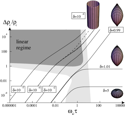
Figure 3: A numerical treatment of the magnetoresistance for arbitrary fields and Fermi surface topologies. These are computed using the results of Eqs. (28) to (33). In the limit of $\delta\gg 1$ the magnetoresistance vanishes as expected in limit of a spheroidal Fermi surface. The previously known asymptotic regimes are unshaded [always $B^{2}$ at weak fields with a high-field asymptote that is $B^{2}$ for open Fermi surfaces ($\delta<1$) or saturates for a closed Fermi surface ($\delta>1$).] The linear regime is heavily shaded while the crossovers are lightly shaded. The dashed line shows the result (for $\delta=10^{-4}$) from the lowest Fourier component of the open orbits [Eq. (34)]. Adding a numerical factor based on the asymptotic limit from all orbits [Eq. (35)] is also shown for this $\delta$ but is indistinguishable from the numerical result. Note that $\delta<10^{-2}$ for all three bands of ${\rm Sr_{2}RuO_{4}}$.

For completeness we consider also the Hall resistivity with current along $c$ and the Hall voltage being developed along the $b$ direction. We find

$$\rho_{H}={-\sigma_{bc}\over\sigma_{bb}\sigma_{cc}+\sigma_{bc}^{2}}\simeq-{eB\tau\over m_{\circ}\sigma_{bb}}\;.$$ (36)

Thus there is no anomalous regime in the Hall resistivity, which remains linear at all magnetic fields and reflects the carrier concentration in the usual way.

IV Comparison with experiment

${\rm Sr_{2}RuO_{4}}$ is probably the best characterized two-dimensional metal. The current experimental $c$-axis magnetoresistance hussey_1997 clearly shows the linear magnetoresistance regime we have discussed [see Fig. (4)]. We now discuss what quantitative information we may determine from this.

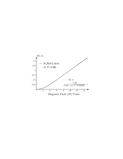
Figure 4: The transverse $c$-axis magnetoresistance of ${\rm Sr_{2}RuO_{4}}$ (data after Hussey et al., Ref. hussey_1997, ). This clearly shows the linear regime we have predicted. The development of the regime at relatively low values of $\Delta\rho_{c}/\rho_{c}\sim 0.2$ as opposed to $\sim 1$ is an indication that more than one band with differing mean-free-paths are involved in the $c$-axis conductivity. This is demonstrated by the fit, which includes a band with low c-axis conductivity and short mean-free-path. This is consistent with the band structure (Ref. bergemann_1999, ) and the Hall coefficient (Ref. hallsr214, ).

Detailed de Haas van Alphen studies give a very clear picture of the degree of warping of the Fermi-surface sheets bergemann_1999 . These are expressed as variations in the radius of the Fermi surface in the $xy$ plane as the Brillouin zone is traversed along the $z$ direction. To translate to our notation we note that

$${\Delta k_{F}\over k_{F}}\simeq{2t_{\perp}\over\epsilon_{F}}={\delta\over 2}\;.$$ (37)

In general, terms in the $c$-axis dispersion can involve $\cos(\nu k_{z}c)$ where $\nu$ is an integer. Thus far we have considered $\nu=1$. Terms with $\nu>1$ increase the $c$-axis conductivity which depends on the square of the $c$-axis velocity ($\sim\nu^{2}$). Furthermore, there can also be an angular variation of the $c$-axis dispersion, $t_{\perp}$, within the plane. This not only modifies the numerical prefactor in the conductivity but generally means that the $c$-axis magnetoresistance becomes dependent on the orientation of the field within the $ab$ plane. This is known to be important in the cuprate superconductors xiang_1996 . Finally, for the particular case of ${\rm Sr_{2}RuO_{4}}$, there are three bands which give additive contributions to the total conductivity.

Because of the three bands and angular variation of $t_{\perp}$, it is misleading to use the formulas we have developed to determine a quantitative measure of Fermi-surface anisotropy from the magnetoresistance. Indeed we have argued that the magnetoresistance becomes universal for each band in the $\delta\rightarrow 0$ limit. Instead we can use the experiments as a probe of in-plane properties—the mean-free-path.

To obtain a good fit to data while introducing a minimum of free parameters, we consider

$$\sigma_{cc}(B)=\beta_{1}+{\beta_{2}\over\sqrt{1+\alpha^{2}_{1}B^{2}}}\;.$$ (38)

This represents one fluid of electrons ($\beta_{1}$) with a short mean-free-path, $l\ll l_{B}^{2}/c$, and therefore insensitive to the fields, and second ($\beta_{2}$) with a much longer mean-free-path [following Eq. (10)]. The magnetoresistance depends only on $\beta_{1}/\beta_{2}\sim 0.1$ and $\alpha_{1}\sim\sqrt{0.04}$. This is consistent with de Haas van Alphen measurements bergemann_1999 which suggest that one Fermi surface sheet, $\gamma$, is considerably less dispersive in the $c$-direction than the other two. In addition, the assumption of a small mean-free-path on that sheet is also consistent with the Hall coefficient that remains strongly temperature dependent in the regime of this experiment hallsr214 . $\alpha_{1}$ may be related to the mean-free-path using $l_{\circ}=\alpha_{1}\hbar/ec$ which gives a value of $l_{\circ}\sim 2000$Å at 3K on the two sheets with the most z-axis dispersion. This is consistent with the observation of unconventional superconductivity in this sample at around $1K$ scsr214 .

V Conclusion

So to summarize: we have given an exact solution for electrical transport within a quasi 2D band structure. In doing so we find that the new dimensionless parameter $\delta=4t_{\perp}/\epsilon_{F}$ is important. This leads to a new region ($\sqrt{\delta}\lesssim\omega_{c}\tau\lesssim 1$) in the magnetoresistance where the $c$-axis transverse magnetoresistance is large $(\Delta\rho_{c}/\rho_{c}\gtrsim 1)$ and linear in the applied field. An asymptotically exact expression for the magnetoresistance has been obtained in the limit of small $\delta$, i.e. the limit of weakly coupled 2D planes. This new region has been observed at low temperatures in the quasi 2D metal $\rm Sr_{2}RuO_{4}$. For the over-doped thallium cuprate there are signs that one is beyond the low field regime at 11 Tesla hussey2 .

VI Acknowledgements

Some of the work described in this paper was done in collaboration with J. M. Wheatley. We have also benefitted from numerous discussions with N. E. Hussey, D. E. Khmelnitskii, A. P. Mackenzie and A. J. Millis. On completion of this work we became aware of a related paper by Lebed and Bagmet lebed . This work complements their approach by computing an analytic expression for the magnetoresistance and including the effect of closed orbits.

References

- (1) P. W. Anderson, Science, 256, 1526 (1992).
- (2) A. P. Mackenzie, et al., Phys. Rev. Lett., 76, 3786 (1996).
- (3) P. L. Kapitza, Proc. Roy. Soc. London A123, 292 (1929).
- (4) A. A. Abrikosov, Introduction to the Theory of Normal Metals, Academic, New York, (1972).
- (5) A. B. Pippard, Magnetoresistance in Metals, Cambridge University Press, Cambridge (1989), and references therein.
- (6) See R. G. Chambers in The Physics of Metals: 1, Electrons, edited J. M. Ziman, Cambridge University Press, Cambridge (1969).
- (7) N. E. Hussey, A. P. Mackenzie, and J. R. Cooper, Y. Maeno and S. Nishizaki, T. Fujita, Phys. Rev. B 57, 5505 (1998).
- (8) We must be careful in calling these cyclotron frequencies because there is no longer a single frequency characterizing the motion. Each Fermi-surface orbit has its own periodicity. Only in the limit of a spheroidal Fermi surface do these frequencies become equal for all orbits. With a single relaxation-time for the metal, the Hall angle () is then independent of position over the Fermi surface. It therefore has no variance so the magnetoresistance is identically zero as shown by N. P. Ong and collaborators in J. M. Harris et al., Phys. Rev. Lett. 75, 1391 (1995).
- (9) Stephen Wolfram, The Mathematica Book—Version 4, Cambridge University, Cambridge (1999), pages 773-776.
- (10) M. Abramowitz and I. A. Stegun, Handbook of Mathematical Functions, Dover, New York (1972).
- (11) I. S. Gradshteyn and A. M. Ryzhik, Table of integrals, series and products, Academic, New York (1965).
- (12) C. Bergemann, S. R. Julian, A. P. Mackenzie, S. Nishizaki and Y. Maeno, Phys. Rev. Lett. 84, 2662 (2000).
- (13) A. P. Mackenzie et al., Phys. Rev. B, 54, 7425, (1996).
- (14) T. Xiang and J. M. Wheatley Phys. Rev. Lett. 77, 4632 (1996).
- (15) Y. Maeno et al. Nature (London) 372, 532 (1994).
- (16) N. E. Hussey, J. R. Cooper, J. M. Wheatley, I. R. Fisher, A. Carrington, A. P. Mackenzie, C. T. Lin and O. Milat, Phys. Rev. Lett. 76, 122 (1996).
- (17) A. G. Lebed and N. N. Bagmet, Phys. Rev. B 55, R8654 (1997).