Nucleation and Growth of the Superconducting Phase in the Presence of a Current

Abstract

We study the localized stationary solutions of the one-dimensional time-dependent Ginzburg-Landau equations in the presence of a current. These threshold perturbations separate undercritical perturbations which return to the normal phase from overcritical perturbations which lead to the superconducting phase. Careful numerical work in the small-current limit shows that the amplitude of these solutions is exponentially small in the current; we provide an approximate analysis which captures this behavior. As the current is increased toward the stall current $J^{*}$, the width of these solutions diverges resulting in widely separated normal-superconducting interfaces. We map out numerically the dependence of $J^{*}$ on $u$ (a parameter characterizing the material) and use asymptotic analysis to derive the behaviors for large $u$ ($J^{*}\sim u^{-1/4}$) and small $u$ ($J\rightarrow J_{c}$, the critical deparing current), which agree with the numerical work in these regimes. For currents other than $J^{*}$ the interface moves, and in this case we study the interface velocity as a function of $u$ and $J$. We find that the velocities are bounded both as $J\rightarrow 0$ and as $J\rightarrow J_{c}$, contrary to previous claims.

]

I Introduction

When a superconductor is placed in a magnetic field equal to its critical field $H_{c}$, the normal and superconducting phases can coexist in a state of equilibrium with the two phases separated by normal-superconducting (NS) interfaces. The dynamics of such interfaces is important for various nonequilibrium phenomena. For instance, if the applied magnetic field is quenched below $H_{c}$, these interfaces move through the sample, expelling the magnetic flux so as to establish the Meissner phase [5, 6, 7, 8, 9, 10, 11, 12, 13]. Just as superconductivity can be destroyed by applying a magnetic field exceeding $H_{c}$, it can also be destroyed by applying a current exceeding the critical depairing current $J_{c}$. Thus by analogy with the magnetic field case, one might expect a special value of the applied current $J^{*}<J_{c}$ at which the superconducting and normal phases coexist, separated by a stationary NS interface [14]. In contrast to the magnetic field induced NS interfaces, these current-induced NS interfaces are intrinsically nonequilibrium entities, and their structure depends upon the dynamics of the order parameter and magnetic field. The evolution and dynamics of these nonequilibrium interfaces is the subject of this paper.

The current-induced NS interfaces arise in several contexts. First, they are known to be important in understanding the dynamics of the “resistive state” in superconducting wires and films (for a review see [15]), and in determining the global stability of the normal and superconducting phases in the presence of a current [16]. Second, Aranson et al. [17] have recently studied the nucleation of the normal phase in thin type-II superconducting strips in the presence of both a magnetic field and a transport current. They found that a sufficient current produced large normal droplets containing multiple flux quanta. Without a current one finds stationary, singly quantized vortices, with a larger amount of NS interface per flux quantum than a multiply quantized droplet. They conclude that the current produces an effective surface tension for the NS interface which is positive, stabilizing the interface and producing larger droplets with smaller surface area. Motivated in part by its role in this phenomenon we wanted to re-examine the nonequilibrium stabilizing effects of current.

Even when the superconducting phase is ostensibly the equilibrium phase, a current makes the normal phase metastable, i.e., linearly stable to infinitesimal superconducting perturbations. A localized superconducting perturbation of finite amplitude, on the other hand, has one of two fates: (1) its amplitude may ultimately shrink to zero restoring the normal phase (undercritical) or (2) it may grow eventually establishing the superconducting state (overcritical). Separating these two possibilities are the critical nuclei or threshold perturbations, for present purposes stationary solutions of the time-dependent Ginzburg-Landau (TDGL) equations localized around the normal state. As one raises the current, the amplitude of the threshold solution grows, implying that the normal phase becomes increasingly stable.

At very low currents, the widths of the critical nuclei shrink as the current is increased, but eventually this trend is reversed and the width grows as the current is increased further. In fact, as the current approaches a particular value, $J^{*}$ (the “stall current”[17]), the width diverges resulting in two well-separated, stationary NS interfaces. The interface solutions have been studied numerically by Likharev [14], who found that the interfaces were stationary at $J^{*}\approx 0.335$ for $u=5.79$, where $u$ characterizes the material and is $5.79$ for nonmagnetic impurities[18]. They were also studied by Kramer and Baratoff [16], who found $J^{*}\approx 0.291$ for $u=12$ (corresponding to paramagnetic impurities[19]). However, we know of no systematic study of the dependence of $J^{*}$ upon $u$. In this work we remedy this situation by using a combination of numerical methods and analysis including matched asymptotic expansions [20]. We show that $J^{*}\sim u^{-1/4}$ for large $u$ in contrast to a previous conjecture [14], and we find how $J^{*}$ approaches $J_{c}$ in the small-$u$ limit.

At currents other than $J^{*}$, the interfaces move with a constant velocity with the superconducting phase invading the normal phase for $J<J^{*}$ and vice versa for $J^{*}<J<J_{c}$. At currents close to $J^{*}$, the interface velocity is proportional to $(J-J^{*})$. Likharev [14] defined the constant of proportionality, $\eta=(dc/dJ)^{-1}|_{J=J^{*}}$, where $c$ is the interface speed; he found $\eta\approx 0.7$ for $u=5.79$. In the extreme limits, $J\rightarrow 0$ and $J\rightarrow J_{c}$ Likharev predicted that the speed $c$ diverges. We find $c$ to be bounded in both cases and provide an analytic expression for it as $J\rightarrow 0$.

The results of this work are summarized in Table I. The rest of the paper is organized as follows. After briefly reviewing the TDGL equations and the approximations used in this work (section II), we study the critical nuclei focusing on their size and shape in the limit $J\rightarrow 0$ (section III). We then move on to consider the stationary interface solutions; in particular we map out the dependence of the stall current $J^{*}$ on $u$ and supplement the numerical work with analysis of the $u\rightarrow\infty$ and $u\rightarrow 0$ limits (section IV). Next, we examine moving interfaces first in the linear response regime and then in the limits $J\rightarrow 0$ and $J\rightarrow J_{c}$ (section V). The appendix contains a calculation of the amplitudes of the critical nuclei in the $J\rightarrow 0$ limit.

TABLE I.: Summary of the primary results.

I. Critical nucleus
Small-$J$ width	$W\sim(uJ)^{-1/2}$	Sec. III B
Small-$J$ amplitude	$\psi_{0}\sim{\rm exp}\{-A/uJ\}$	Sec. III B
II. Stall current $J^{*}$
Large-$u$	$J^{*}=0.584491~{}u^{-1/4}$	Sec. IV C
Small-$u$	$J^{*}=J_{c}{\textstyle(1-u/8)^{1/2}\over\textstyle(1-u/24)^{3/2}}$	Sec. IV D
III. Kinetic coeff. $\eta$
Large-$u$	$\eta=0.797~{}u^{3/4}$	Sec. V
Small-$u$	$\eta\sim u^{3/2}$	Sec. V
IV. Interface speed
$J\rightarrow 0$	$c\rightarrow 2/u$	Sec. V
$J\rightarrow J_{c}$	$c\sim u^{1/2}$     $(u\rightarrow 0)$	Sec. V
	$c\sim u^{-0.85}$   $(u\rightarrow\infty)$	Sec. V

II The TDGL equations

The starting point for our study is the set of TDGL equations for the order parameter $\psi$, the scalar potential $\Phi$, and the vector potential ${\bf A}$:

$$\hbar\gamma\left(\partial_{t}+{ie^{*}\Phi\over\hbar}\right)\psi = \frac{\hbar^{2}}{2m}\left({\mathchoice{{\hbox{\boldmath$\displaystyle\nabla$}}}{{\hbox{\boldmath$\textstyle\nabla$}}}{{\hbox{\boldmath$\scriptstyle\nabla$}}}{{\hbox{\boldmath$\scriptscriptstyle\nabla$}}}}-\frac{ie^{*}{\bf A}}{\hbar c}\right)^{2}\psi$$ (2)

$$+|a|\psi-b|\psi|^{2}\psi,$$

$${\mathchoice{{\hbox{\boldmath$\displaystyle\nabla$}}}{{\hbox{\boldmath$\textstyle\nabla$}}}{{\hbox{\boldmath$\scriptstyle\nabla$}}}{{\hbox{\boldmath$\scriptscriptstyle\nabla$}}}}\times{\mathchoice{{\hbox{\boldmath$\displaystyle\nabla$}}}{{\hbox{\boldmath$\textstyle\nabla$}}}{{\hbox{\boldmath$\scriptstyle\nabla$}}}{{\hbox{\boldmath$\scriptscriptstyle\nabla$}}}}\times{\bf A}=\frac{4\pi}{c}({\bf J}_{n}+{\bf J}_{s}),$$ (3)

where the normal current ${\bf J}_{n}$ and the supercurrent ${\bf J}_{s}$ are given by

$${\bf J}_{n}=\sigma^{(n)}\left(-\partial_{t}{\bf A}/c-{\mathchoice{{\hbox{\boldmath$\displaystyle\nabla$}}}{{\hbox{\boldmath$\textstyle\nabla$}}}{{\hbox{\boldmath$\scriptstyle\nabla$}}}{{\hbox{\boldmath$\scriptscriptstyle\nabla$}}}}\Phi\right),$$ (6)

$${\bf J}_{s}={\hbar e^{*}\over 2mi}\left(\psi^{*}{\mathchoice{{\hbox{\boldmath$\displaystyle\nabla$}}}{{\hbox{\boldmath$\textstyle\nabla$}}}{{\hbox{\boldmath$\scriptstyle\nabla$}}}{{\hbox{\boldmath$\scriptscriptstyle\nabla$}}}}\psi-\psi{\mathchoice{{\hbox{\boldmath$\displaystyle\nabla$}}}{{\hbox{\boldmath$\textstyle\nabla$}}}{{\hbox{\boldmath$\scriptstyle\nabla$}}}{{\hbox{\boldmath$\scriptscriptstyle\nabla$}}}}\psi^{*}\right)-\frac{e^{*2}}{mc}|\psi|^{2}{\bf A},$$

and where $\gamma$ (which is assumed to be real) is a dimensionless quantity characterizing the relaxation time of the order parameter, $\sigma^{(n)}$ is the normal conductivity, and $a=a_{0}(1-T/T_{c0})$. From these parameters we can form two important length scales, the coherence length $\xi=\hbar/(2m|a|)^{1/2}$ and the penetration depth $\lambda=[mbc^{2}/4\pi(e^{*})^{2}|a|]^{1/2}$.

These equations assume relaxational dynamics for the order parameter as well as a two-fluid description for the current. With somewhat restrictive assumptions, they can be derived from the microscopic BCS theory [18, 19]. Further simplification is possible in the limit of a thin, narrow film, that is, when the thickness is less than the coherence length, $d<\xi$, and the width is less than the effective penetration depth [21], $w\ll\lambda^{2}/d$. In this case the current carried by the film or wire is small, and we needn’t worry about the fields it produces. Therefore, Eq. (3) may be dropped, and we need only specify the total current ${\bf J}={\bf J}_{n}+{\bf J}_{s}$ (subject to ${\mathchoice{{\hbox{\boldmath$\displaystyle\nabla$}}}{{\hbox{\boldmath$\textstyle\nabla$}}}{{\hbox{\boldmath$\scriptstyle\nabla$}}}{{\hbox{\boldmath$\scriptscriptstyle\nabla$}}}}\cdot{\bf J}=0$), along with the order-parameter dynamics, Eq. (2). This approximation is commonly used for superconducting wires [15] and can be justified mathematically for superconducting films [22]. In addition, we will be considering processes in the absence of an applied magnetic field, so that we may set ${\bf A}={\bf 0}$. With these simplifications, we can now rewrite the equations in terms of dimensionless (primed) quantities,

$$\psi=\sqrt{{|a|\over b}}\psi^{\prime},\ \ \ \ \ \ \Phi={\hbar e^{*}|a|\over mb\sigma^{(n)}}\mu^{\prime},$$ (7)

$$x=\xi x^{\prime},\ \ \ \ \ \ t={mb\sigma^{(n)}\over e^{*2}|a|}t^{\prime},$$ (8)

$$J=\sqrt{{2\over m}}{e^{*}|a|^{3/2}\over b}J^{\prime},\ \ \ \$$ (9)

which leads to

$$u(\partial_{t^{\prime}}+i\mu^{\prime})\psi^{\prime}=(\nabla^{\prime 2}+1-|\psi^{\prime}|^{2})\psi^{\prime},$$ (11)

$${\bf J^{\prime}}={\rm Im}(\psi^{\prime*}{\mathchoice{{\hbox{\boldmath$\displaystyle\nabla$}}}{{\hbox{\boldmath$\textstyle\nabla$}}}{{\hbox{\boldmath$\scriptstyle\nabla$}}}{{\hbox{\boldmath$\scriptscriptstyle\nabla$}}}}^{\prime}{\psi^{\prime}})-{\mathchoice{{\hbox{\boldmath$\displaystyle\nabla$}}}{{\hbox{\boldmath$\textstyle\nabla$}}}{{\hbox{\boldmath$\scriptstyle\nabla$}}}{{\hbox{\boldmath$\scriptscriptstyle\nabla$}}}}^{\prime}{\mu}^{\prime},\quad{\mathchoice{{\hbox{\boldmath$\displaystyle\nabla$}}}{{\hbox{\boldmath$\textstyle\nabla$}}}{{\hbox{\boldmath$\scriptstyle\nabla$}}}{{\hbox{\boldmath$\scriptscriptstyle\nabla$}}}}^{\prime}\cdot{\bf J^{\prime}}=0.$$ (12)

Note that length is measured in units of coherence length [23]. We will drop the primes hereafter. The only parameters remaining in the problem are the scaled current $J$ and a dimensionless material parameter $u=\tau_{\psi}/\tau_{J}$, where $\tau_{\psi}=\hbar\gamma/|a|$ is the order-parameter relaxation time and $\tau_{J}=\sigma^{(n)}mb/e^{*2}|a|$ is the current relaxation time. We will treat $u$ as a phenomenological parameter and study the nucleation and growth process as a function of $u$. The microscopic derivations of the TDGL equations predict that $u=5.79$ (nonmagnetic impurities) [18], and $u=12$ (paramagnetic impurities) [19], but small $u$ is also useful for modeling gapped superconductors [24].

III Nucleation of the superconducting phase from the normal phase

In the presence of an applied current the normal phase in a wire is linearly stable with respect to superconducting perturbations for any value of the current [25, 26]. The reason for this stability is that any quiescent superconducting fluctuation will be accelerated by the electric field, its velocity eventually exceeding the critical depairing velocity, resulting in the decay of the fluctuation. The growth of the superconducting phase therefore requires a nucleus of sufficient size that will locally screen the electric field and allow the superconducting phase to continue growing; smaller nuclei will simply decay back to the normal phase. The amplitude of the “critical” nucleus should decrease as the current approaches zero, reaching zero only at $J=0$. We expect the critical nuclei to be unstable, stationary (but nonequilibrium) solutions of the TDGL equations, which asymptotically approach the normal solution as $x\rightarrow\pm\infty$. These “bump” solutions of the TDGL equations are the subject of this section. We include here an extensive numerical study of the amplitudes and widths of the critical nuclei, as well as some analytical estimates for these quantities.

A Numerical results

Let us start by discussing the numerical work on the critical nuclei. For the analytic work, we often find it convenient to use the amplitude and phase variables, i.e. $\psi=f{\rm e}^{i\theta}$; but they are ill-suited for the numerical work, since the calculation of the phase becomes difficult when the amplitude is small. Following Likharev [14] we use instead $\psi=R+iI$, with $R$ and $I$ real, and in one dimension Eqs. (II) become

$$uR_{t} = R_{xx}+u\mu I+R-(R^{2}+I^{2})R,$$ (14)

$$uI_{t} = I_{xx}-u\mu R+I-(R^{2}+I^{2})I,$$ (15)

$$J = RI_{x}-IR_{x}-\mu_{x}.$$ (16)

Since the nuclei are unstable stationary states, they are investigated only by time-independent means. Such solutions require a particular gauge choice—in this case $\mu(x)=0$ where $\psi(x)$ has its maximum amplitude; they are then sought using a relaxation algorithm [27]. Figure 1 shows a typical bump’s amplitude, $f=\sqrt{R^{2}+I^{2}}$, the associated superfluid velocity $q=(RI_{x}-IR_{x})/f^{2}$ and the electric field $E(x)=-\mu_{x}(x)$. The figure shows only half of the solution; $f(x)$, $q(x)$ and $E(x)$ are even about $x=0$. In Fig. 2 we plot the bump’s maximum amplitude, $\psi_{0}$, as a function of $J$; it grows as the current rises, indicating the increasing stability of the normal phase. In the data presented by Watts-Tobin et al. [28] $\psi_{0}$ appears to vary linearly with $J$ for small $J$. However, in our numerical calculations at very small currents the dependence deviates from linearity (see the inset of Fig. 2), and $\psi_{0}$ drops rapidly to zero as $J\rightarrow 0$, consistent with the exponential behavior suggested in Refs. [15, 29]. More precisely our small-$J$ data ($0.008\leq J\leq 0.015$) at $u=5.79$ is fit by

$$\psi_{0}(J)=B\exp(-A/uJ),$$ (17)

with $A=0.042$ and $B=0.19$. A somewhat similar dependence (with $A=2/3$) was suggested by Ivlev et al. [15, 29]; they were considering a distinct quantity but one also related to critical fluctuations about the normal phase (see the Appendix for more details).

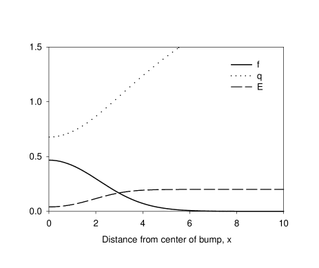
FIG. 1.: The bump’s amplitude, $f(x)$, its superfluid velocity, $q(x)$, and the electric field, $E(x)$, for $u=5.79$ and $J=0.2$.

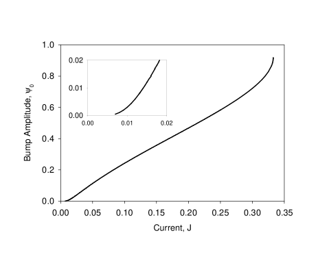
FIG. 2.: The maximum amplitude of the bumps $\psi_{0}$ as a function of $J$ for $u=5.79$. The inset shows the exponential dependence of the small-$J$ data, see Eq. (17).

The width of the bump diverges in the small-$J$ limit like $(uJ)^{-1/2}$, as can be seen from the analysis below. So as $J$ is increased from zero, the width initially shrinks, but eventually the width begins to grow again, diverging as the current approaches the stall current $J^{*}$. In this limit the bump transforms into two well separated interfaces (see Fig. 3).

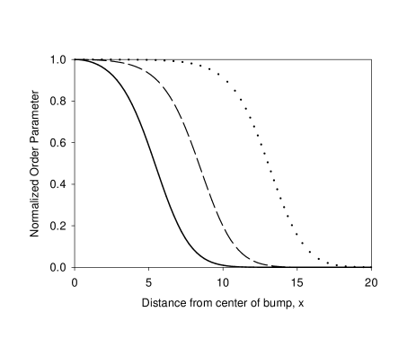
FIG. 3.: The bump profiles for $J^{*}-J=10^{-3}$ (solid), $J^{*}-J=10^{-5}$ (dashed) and $J^{*}-J=10^{-7}$ (dotted) at $u=5.79$.

B Analysis in the $J\rightarrow 0$ limit

The equations for nuclei centered at the origin are

$$\psi_{xx}-iu\mu\psi+\psi-|\psi|^{2}\psi=0,$$ (19)

$$\mu=-Jx+\int_{0}^{x}{\rm Im}\left(\psi^{*}\psi_{x^{\prime}}\right)dx^{\prime},$$ (20)

where we have dropped the term $\psi_{t}$ and selected the gauge $\mu(0)=0$. We saw in Fig. 2 that $\psi_{0}$ becomes very tiny in the small-$J$ limit, thus the nonlinear terms can be neglected, leading to

$$\psi_{xx}+iuJx\psi+\psi=0,$$ (21)

a complex version of the Airy equation. Applying the WKB method results in the approximate solution

$$\psi\sim [1+(uJx)^{2}]^{-1/8}$$ (22)

$$\times \exp\left\{\frac{2}{3\,uJ}\left[\left[1+(uJx)^{2}\right]^{3/4}\cos\frac{3\alpha}{2}-1\right]\right\}$$ (23)

$$\times \exp\left\{i\left[\frac{2}{3\,uJ}\left[1+(uJx)^{2}\right]^{3/4}\sin\frac{3\alpha}{2}-\frac{\alpha}{4}\right]\right\},$$ (24)

where $\alpha=\tan^{-1}(uJx)$. The numerical data agrees quite well with this predicted shape in the small-$J$ limit. For small $x$ the expression can be approximated by

$$\psi\sim\exp\left[i(1-uJ/4)x-uJx^{2}/4\right].$$ (25)

We see here that the width of the bump varies like $(uJ)^{-1/2}$ in this limit and that the superfluid velocity $q\approx(1-uJ/4)$. For large $x$, on the other hand, where $\alpha\approx\pi/2$, the expression becomes

$$\psi\sim(uJx)^{-1/4}\exp\left[-{\sqrt{2uJ}\over 3}|x|^{3/2}(1-i)\right],$$ (26)

as one expects for the Airy function. Note that deep in the tail of the solution, we see a different length scale $\lambda_{Airy}\sim(uJ)^{-1/3}$ arising.

Since the above analysis is of a linear equation, it can not determine the amplitude of the nucleus; for this purpose the nonlinearities must be considered. In the appendix we outline an ad hoc calculation of the small-$J$ limit of the bump amplitude. We take a $\psi$ of an unknown amplitude but of a fixed shape inspired by the above analysis and assume that it is a stationary solution of the full TDGL. We then determine its amplitude self-consistently. The resulting amplitude is

$$|\psi|\approx\left(\frac{2J}{\pi u}\right)^{1/4}\left(\frac{9}{8}-\frac{1}{u}\right)^{-1/2}\exp\left(-\frac{16}{81~{}uJ}\right).$$ (27)

The factor $A=16/81$ is within a few percent of that extracted from the numerical data.

IV Stationary Interfaces

As the current is raised, the width of the critical nucleus grows and ultimately diverges as the stall current is reached, resulting in well separated, stationary interfaces. These interface solutions will be the subject of the rest of this work.

A Numerical methods and results

Let us first discuss the numerical work on the interface solutions. For given values of $u$ and $J$ we evolved the TDGL equations from an initial guess which is purely superconducting on the left, $\psi(x)=f_{\infty}~{}{\rm e}^{iq_{\infty}x}$ and $\mu_{x}(x)=0$, and purely normal on the right, $\psi(x)=0$ and $\mu_{x}(x)=-J$. The values $f_{\infty}$ and $q_{\infty}$ are related to the applied current through

$$J = f_{\infty}^{2}\sqrt{1-f_{\infty}^{2}},$$ (29)

$$q_{\infty} = \sqrt{1-f_{\infty}^{2}}.$$ (30)

Stability requires taking the larger positive root of the former equation [30] which places the following bounds on $J$, $f_{\infty}$ and $q_{\infty}$:

$$0\leq J\leq J_{c}=\sqrt{4/27}\approx 0.3849,$$ (32)

$$1\geq f_{\infty}\geq\sqrt{2/3}\approx 0.8165,$$ (33)

$$0\leq q_{\infty}\leq\sqrt{1/3}\approx 0.5774.$$ (34)

We employed several schemes to integrate the equations in time including both explicit (Euler) and implicit (Crank-Nicholson) [27].

Initially the front moves and changes shape but eventually it reaches a steady state in which the interface moves at a constant velocity without further deformation. By the time-dependent means we found locally stable, constant-velocity solutions for currents less than $J_{c}$. To examine these solutions more accurately, we adopted a time-independent method. First, we transformed coordinates to a moving frame, $x^{\prime}=x-ct$; next, we chose $\mu=cq_{\infty}$ as $x\rightarrow-\infty$ which allows for a truly time-independent solution (i.e. one with both amplitude and phase time-independent). Then we searched for stationary solutions using a relaxation algorithm [27] where ($u,J$) are input parameters and $c$ is treated as an eigenvalue. This approach requires an additional boundary condition to fix translational invariance; we elected to fix $\mu$ on the rightmost site. To find the stall currents $J^{*}$ we can set $c=0$ and take $J$ or $u$ as the eigenvalue.

Figures 4 and 5 show the order-parameter amplitude $f$ and the electric-field distribution $E=-\mu_{x}$ of the stalled interface determined for $u=500$ and $u=1.04$ respectively. Note that while $f$ is very flat in the superconducting region, the real and imaginary parts, $R$ and $I$, oscillate with a wavelength $2\pi/q_{\infty}$. Because of this additional length scale inherent in $R$ and $I$, there is little to be gained from varying the mesh size. In fact, this length scale is compressed as we move to the right, and we are only saved from the difficulties of handling rapidly oscillating functions by the fact that the amplitudes decay so quickly.

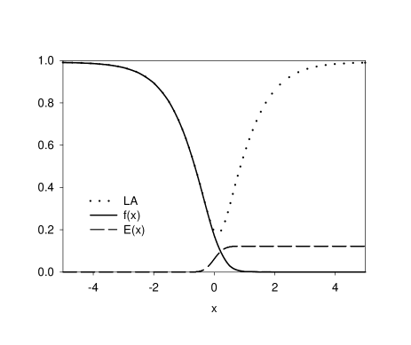
FIG. 4.: The stationary NS interface solution when $u=500$ for which the stall current $J^{*}=0.12252$. Shown here are the numerically determined $f(x)$ and $E(x)$, as well as the Langer-Ambegaokar (LA) solution (Eq. (54), the solution with no electric field) corresponding to the same current.

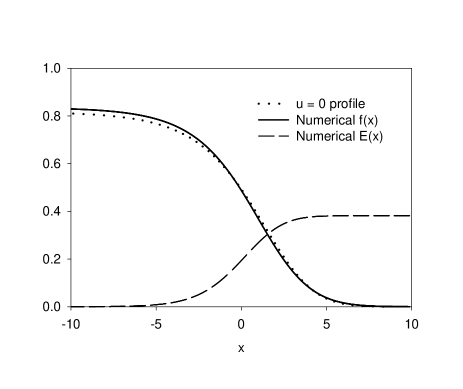
FIG. 5.: The stationary NS interface solution when $u=1.04$ for which the stall current $J^{*}=0.3836$. Shown here are the numerically determined $f(x)$ and $E(x)$, as well as the function ${\hat{f}}_{0}(\hat{x})$, the $u\rightarrow 0$ profile, derived from Eq. (91) where $\hat{x}=u^{1/2}x$.

In the large-$u$ case (see Fig. 4), $E(x)$ remains flat throughout most of the space; it changes abruptly from one constant to another only after $f(x)$ has become small. The variations of $f(x)$ are more gradual; however, the greatest changes in $f_{x}$ occur in that same small area. This region of rapid change is known as a boundary layer; it marks where the current suddenly changes from superconducting to normal, i.e., the position of the NS interface. As $u$ increases, the longer length scale over which $f$ varies on the superconducting side remains essentially fixed, while the boundary-layer thickness shrinks to zero. In the opposite limit, the small-$u$ case (see Fig. 5), $f(x)$ and $E(x)$ appear to vary together even in the superconducting region; moreover, the length scale over which they vary grows as $u$ is decreased. We will postpone providing more of the numerical results on the interfaces until some of the analytic arguments are available for comparison.

B Asymptotic analysis of the interface solutions: preliminaries

Before addressing the large-$u$ and small-$u$ limits separately, let us put the TDGL equations into a form convenient for analysis and derive expressions for the length scales deep in the superconducting and normal regions. The disparity of these length scales in the large-$u$ limit will motivate the boundary-layer analysis in that regime; while an inequality they satisfy will lead to the conclusion that $J^{*}\rightarrow J_{c}$ in the small-$u$ limit.

We make the substitution $\psi=fe^{i\theta}$, which yields

$$uf_{t}=f_{xx}-f(\theta_{x})^{2}+f-f^{3},$$ (36)

$$u(\theta_{t}+\mu)f=2f_{x}\theta_{x}+f\theta_{xx},$$ (37)

$$J=f^{2}\theta_{x}-\mu_{x}.$$ (38)

Next we restrict our attention to stationary solutions. Note that only spatial derivatives of $\theta$ appear now, allowing us to work with the superfluid velocity $q=\theta_{x}$ instead of $\theta$. The equations become

$$f_{xx}-q^{2}f+f-f^{3}=0,$$ (40)

$$u\mu f=2f_{x}q+fq_{x},$$ (41)

$$J^{*}=f^{2}q-\mu_{x},$$ (42)

where $J^{*}$ replaces $J$ as these equations apply to the stall situation. Next multiply Eq. (41) by $f$ and note that the right hand side is now $(f^{2}q)_{x}$ which we can express in terms of $\mu$ by differentiating Eq. (42); these steps lead to

$$\mu_{xx}=uf^{2}\mu.$$ (43)

Now let us assume the following asymptotic forms as $x\rightarrow-\infty$:

$$\lim_{x\to-\infty}f(x) = f_{\infty}-f_{1}~{}{\rm e}^{x/\lambda_{f}}+\ldots,$$ (45)

$$\lim_{x\to-\infty}q(x) = q_{\infty}+q_{1}~{}{\rm e}^{x/\lambda_{q}}+\ldots,$$ (46)

$$\lim_{x\to-\infty}\mu(x) = \mu_{\infty}-\mu_{1}~{}{\rm e}^{x/\lambda_{\mu}}+\ldots.$$ (47)

Substituting these expressions into Eqs. (40), (42) and (43) and recalling the boundary conditions yields

$$\left(2f_{\infty}^{2}-\lambda_{f}^{-2}\right)f_{1}{\rm e}^{x/\lambda_{f}}-2f_{\infty}q_{\infty}q_{1}{\rm e}^{x/\lambda_{q}}=0,$$ (51)

$$-2f_{\infty}q_{\infty}f_{1}{\rm e}^{x/\lambda_{f}}+f_{\infty}^{2}q_{1}{\rm e}^{x/\lambda_{q}}+\lambda_{\mu}^{-1}\mu_{1}{\rm e}^{x/\lambda_{\mu}}=0,$$

$$\lambda_{\mu}^{-2}-uf_{\infty}^{2}=0.$$

Eq. (51) provides an expression for $\lambda_{\mu}$, the electric-field screening length. Since $f_{\infty}$ is always of $O(1)$, we see that $\lambda_{\mu}$ shrinks as $u\rightarrow\infty$ and diverges as $u\rightarrow 0$, which is consistent with the behavior seen in Figs. 4 and 5.

More than one decay length appears in Eqs. (51) and (51). If they are not equal, the term with the shorter length is exponentially small compared to the other(s) and will not contribute to the $x\rightarrow-\infty$ limit. Since none of the terms in Eq. (51) can equal zero individually, we conclude that the longer two of $\lambda_{f}$, $\lambda_{q}$ and $\lambda_{\mu}$ must be equal. Next, because the term multiplying ${\rm e}^{x/\lambda_{q}}$ in Eq. (51) cannot equal zero on its own, we determine that $\lambda_{q}\leq\lambda_{f}$, making $\lambda_{f}$ one of the longer lengths. Finally, if we assume that $\lambda_{f}=\lambda_{\mu}>\lambda_{q}$ we find that $\lambda_{f}=2^{-1/2}f_{\infty}^{-1}$ and $\lambda_{\mu}=u^{-1/2}f_{\infty}^{-1}$ and reach a contradiction (except at $u=2$). Thus provided the original assumption of an exponential approach is valid, we conclude that

$$\lambda_{f}=\lambda_{q}\geq\lambda_{\mu}.$$ (52)

This equality of $\lambda_{f}$ and $\lambda_{q}$ is reasonable given that both $f$ and $q$ are related to the complex order parameter $\psi$. Also, having $\lambda_{f}>\lambda_{\mu}$ is consistent with the large-$u$ data seen in Fig. 4. If $\lambda_{\mu}\neq\lambda_{f}$ then

$$\lambda_{f}^{-2}=6f_{\infty}^{2}-4=\lambda_{LA}^{-2}.$$ (53)

We identify this length scale as $\lambda_{LA}$ since it coincides with that occurring in the solution of Eqs. (IV B) without any electric field ($\mu(x)=0$),

$$f^{2}(x)=f_{\infty}^{2}-(3f_{\infty}^{2}-2)~{}{\rm sech}^{2}\left(\sqrt{\frac{3f_{\infty}^{2}-2}{2}}x\right),$$ (54)

which was found by Langer and Ambegaokar [30] in their study of phase slippage. The asymptotic form of Eq. (54) looks like Eq. (45) with $\lambda_{f}$ given by Eq. (53). As a matter of fact because $\lambda_{f}\gg\lambda_{\mu}$ in the large-$u$ limit, the profile of $f(x)$ is only imperceptibly different from the Langer-Ambegaokar (LA) solution in the superconducting region and deviates from it only in the boundary layer, as is shown in Fig. 4.

Recall that $\lambda_{\mu}$ diverges as $u\rightarrow 0$; the inequality $\lambda_{f}\geq\lambda_{\mu}$ implies that $\lambda_{f}$ must diverge as fast or faster in this limit. This scenario is consistent with the small-$u$ data shown in Fig. 5 in which $f(x)$ and $E(x)$ vary on long length scales. Eq. (53) suggests that a diverging $\lambda_{f}$ implies that $f_{\infty}\rightarrow\sqrt{2/3}$ and in turn that $J\rightarrow J_{c}$ as $u\rightarrow 0$, which is also consistent with what is found numerically.

In the other asymptotic limit, deep in the normal regime, $\psi$ is very small and hence the nonlinear terms in Eqs. (II) can be dropped as was done for the bumps in the small-$J$ limit. The result is a complex Airy equation, the asymptotic analysis of which was supplied in Eq. (26), where we saw the length scale $\lambda_{Airy}\sim(uJ^{*})^{-1/3}$. Somewhat like $\lambda_{\mu}$, $\lambda_{Airy}$ shrinks as $u\rightarrow\infty$ and expands as $u\rightarrow 0$ but with different powers of $u$. The presence of the disparate length scales, $\lambda_{f}$, $\lambda_{\mu}$ and $\lambda_{Airy}$, in the large-$u$ limit motivates the use of the boundary-layer analysis that comes next. We will see that $\lambda_{Airy}$ scales in the same way as the boundary-layer thickness.

C Asymptotic behavior of the stall current as $u\rightarrow\infty$

We have already seen in Fig. 4 that the large-$u$ profile can be divided into two regions—one slowly varying, one rapidly varying, also known as the outer and inner regions, respectively. Furthermore, it has been suggested that the ratio of the length scales characterizing these regions decreases as $u\rightarrow\infty$. These features make the problem ideally suited for boundary-layer analysis, in which one identifies the terms that dominate the differential equation in each region, analyzes the reduced equations consisting of dominant terms and then matches the behavior in some intermediate region.

We start by eliminating the superfluid velocity $q$ from Eqs. (IV B), resulting in

$$f_{xx}-(J^{*}+\mu_{x})^{2}f^{-3}+f-f^{3}=0,$$ (56)

$$\mu_{xx}-uf^{2}\mu=0.$$ (57)

Let us consider first the slowly varying, superconducting region. We saw in the preliminary analysis that for large $u$, $\mu(x)$ is exponentially small, so we drop it. Next, let us assume that $J^{*}$ is small and drop it; we can verify in the end that this is self-consistent. The reduced equation is

$$f_{xx}+f-f^{3}\approx 0,$$ (58)

with solution $f(x)=-{\rm tanh}(x/\sqrt{2})$.

Moving in from the left toward the interface (into the boundary-layer region), $f$ becomes small, and the second term in Eq. (56) which was subdominant becomes dominant. In this inner region $f$ is small but rapidly varying, thus the dominant terms are

$$f_{xx}\approx\frac{(J^{*}+\mu_{x})^{2}}{f^{3}},$$ (59)

along with Eq. (57). Having identified the dominant terms, now we must make certain they balance. We assume that in the boundary layer, all the quantities scale as powers of $u$:

$$f\sim u^{-\alpha},\quad\mu\sim u^{-\beta},\quad J^{*}\sim u^{-\gamma},\quad x\sim u^{-\delta}.$$ (60)

Balancing terms in Eq. (59), we find $2\alpha=\gamma+\delta$, while balancing terms in Eq. (57) yields $2(\alpha+\delta)=1$. Next, we need to ensure that the solutions in the boundary layer match onto the solutions in the superconducting and normal regions. By expanding the superconducting solution near the interface, we see that $f(x)\sim-x/\sqrt{2}$ as the boundary layer is approached; matching to the boundary layer requires $f_{x}\sim 1$, so that $\alpha=\gamma$. In the normal region, $\mu\approx-J^{*}x$, so that matching to the boundary layer requires $\mu_{x}\sim J^{*}$, and $\beta=\gamma+\delta$. Solving this set of equations, we conclude that $\alpha=\gamma=\delta=1/4$ and $\beta=1/2$, i.e., the stall current $J^{*}\sim u^{-1/4}$ for large $u$. Note that $J^{*}\rightarrow 0$ as $u\rightarrow\infty$, so that we were justified in dropping $J^{*2}/f^{3}$ from Eq. (58). Substituting $J^{*}\sim u^{-1/4}$ into $\lambda_{Airy}$ gives $\lambda_{Airy}\sim u^{-1/4}$, indicating that it may be identified as the boundary-layer thickness.

In order to determine the coefficient of the $u^{-1/4}$ in the stall current we need to solve the boundary layer problem. Let us rescale in the way suggested above:

$$f=u^{-1/4}F,\quad\mu=u^{-1/2}M(X),$$ (61)

$$J=u^{-1/4}\tilde{J},\quad x=u^{-1/4}X.$$ (62)

Substituting these rescaled variables into Eqs. (56) and (57), and then expanding $F$, $M$ and $\tilde{J}$ in powers of $u^{-1/2}$, we obtain at the lowest order

$$F_{0,XX}-\frac{({\tilde{J}}_{0}+M_{0,X})^{2}}{F_{0}^{3}}=0,$$ (64)

$$M_{0,XX}-F_{0}^{2}M_{0}=0,$$ (65)

with the boundary conditions (from the outer regions)

$$F_{0,X}(-\infty) =-1/\sqrt{2},\qquad M_{0}(-\infty) =0,$$ (66)

$$F_{0}(+\infty) =0,\qquad M_{0,X}(+\infty) =-{\tilde{J}}_{0}.$$ (67)

(As before we need an extra boundary condition to fix the translational invariance.) For an arbitrary ${\tilde{J}}_{0}$ the solutions of Eqs. (64) and (65) cannot satisfy the boundary conditions; ${\tilde{J}}_{0}$ must be tuned to a particular value before all of the boundary conditions are satisfied, leading to a nonlinear eigenvalue problem for ${\tilde{J}}_{0}$. We have solved this eigenvalue problem numerically and find that ${\tilde{J}}_{0}=0.584491$. Therefore, to leading order we have for the stall current

$$J^{*}\approx 0.584491\,u^{-1/4}.$$ (68)

This prediction agrees well with the numerical results and disagrees with Likharev’s conjecture of a $u^{-1/3}$ dependence [14], as can be seen in Fig. 6 and in Table II. It is in principle possible to carry out this procedure to successively higher orders, but the equations become cumbersome. Instead we have simply opted to fit our numerical data to a form inspired by the asymptotic analysis,

$$J^{*} = 0.584491\,u^{-1/4}-0.117461\,u^{-3/4}-0.12498\,u^{-5/4}$$ (70)

$$+0.163043\,u^{-7/4}+O\left(u^{-9/4}\right).$$

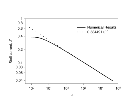
FIG. 6.: A log-log plot of the stall current $J^{*}$ vs. $u$. The solid line shows the numerically determined $J^{*}$’s as a function of $u$ and the dotted line is $0.584491~{}u^{-1/4}$ (the large-$u$ behavior predicted by matched asymptotic analysis).

TABLE II.: Representative numerical results for the stall current $J^{*}$ and kinetic coefficient $\eta$.

$u$	$J^{*}$	$J^{*}u^{1/4}$	$\eta$	$\eta u^{-3/4}$
1	0.3838	0.3838	0.01871	0.01871
5	0.3407	0.5094	0.6400	0.1914
10	0.3013	0.5359	1.573	0.2797
50	0.2127	0.5655	8.258	0.4315
100	0.1807	0.5715	15.59	0.4931
500	0.1224	0.5788	62.51	0.5875
1000	0.1033	0.5807	111.3	0.6259
5000	0.0693	0.5828	407.9	0.6847
10000	0.0583	0.5833	708.4	0.7084
50000	0.0391	0.5840	2487	0.7440

D Asymptotic behavior of the stall current as $u\rightarrow 0$

Now let us examine the opposite limit of $u\rightarrow 0$. In this case the electric-field screening length becomes long, and Ivlev et al. [24] have proposed that this makes the small-$u$ limit useful for modeling gapped superconductors. As already suggested the inequality of length scales, $\lambda_{f}\geq\lambda_{\mu}$ implies that $J^{*}\rightarrow J_{c}$. We will begin our small-$u$ analysis by putting this result on firmer ground and extracting as a byproduct the $u\rightarrow 0$ limit of the interface profile.

The rescaled equations. Recall that deep in the superconducting region $\lambda_{\mu}\sim u^{-1/2}$. This observation suggests that we rescale distance: $x=u^{-1/2}\hat{x}$; furthermore, to ensure that the normal current ($-\mu_{x}$) scales in the same way as the total current we rescale $\mu=u^{-1/2}\hat{\mu}$ as well. These rescalings yield

$$u\hat{f}_{\hat{x}\hat{x}}-{\hat{q}}^{2}\hat{f}+\hat{f}-{\hat{f}}^{3}=0,$$ (72)

$$\hat{\mu}\hat{f}=2\hat{q}{\hat{f}}_{\hat{x}}+\hat{f}{\hat{q}}_{\hat{x}},$$ (73)

$$J^{*}={\hat{f}}^{2}\hat{q}-{\hat{\mu}}_{\hat{x}},$$ (74)

placing the small parameter $u$ in front of ${\hat{f}}_{\hat{x}\hat{x}}$. If we expand these functions as series in powers of $u$

$$\hat{f} = {\hat{f}}_{0}+u{\hat{f}}_{1}+\ldots,$$ (76)

$$\hat{q} = {\hat{q}}_{0}+u{\hat{q}}_{1}+\ldots,$$ (77)

$$\hat{\mu} = {\hat{\mu}}_{0}+u{\hat{\mu}}_{1}+\ldots,$$ (78)

$$J^{*} = J_{0}^{*}+uJ_{1}^{*}+\ldots,$$ (79)

then we find at the lowest order

$$-{\hat{q}}_{0}^{2}{\hat{f}}_{0}+{\hat{f}}_{0}-{\hat{f}}_{0}^{3}=0,$$ (81)

$${\hat{\mu}}_{0}{\hat{f}}_{0}=2{\hat{q}}_{0}{\hat{f}}_{0,x}+{\hat{f}}_{0}{\hat{q}}_{0,x},$$ (83)

$$J_{0}^{*}={\hat{f}}_{0}^{2}{\hat{q}}_{0}-{\hat{\mu}}_{0,\hat{x}}.$$

The solution of Eq. (81) is either ${\hat{f}}_{0}=0$ (the normal phase) or ${\hat{f}}_{0}=(1-{\hat{q}}_{0}^{2})^{1/2}$ (the superconducting phase). Let us focus on the superconducting solutions. By eliminating ${\hat{q}}_{0}$, we obtain the first order equations

$${\hat{f}}_{0,\hat{x}} = \frac{{\hat{f}}_{0}\sqrt{1-{\hat{f}}_{0}^{2}}~{}{\hat{\mu}}_{0}}{2-3{\hat{f}}_{0}^{2}},$$ (85)

$${\hat{\mu}}_{0,\hat{x}} = {\hat{f}}_{0}^{2}\sqrt{1-{\hat{f}}_{0}^{2}}-J_{0}^{*}.$$ (86)

Because ${\hat{f}}_{0}$ ranges from $f_{\infty}$ to $0$ and $f_{\infty}\geq\sqrt{2/3}$, we know that ${\hat{f}}_{0}$ either starts at or passes through $\sqrt{2/3}$. (Strictly speaking we should be writing here $f_{\infty,0}$, the lowest order term in the expansion of $f_{\infty}$.) Thus, the effect of the pole in Eq. (85) must be considered. If it is not canceled by a zero in ${\hat{\mu}}_{0}$, ${\hat{f}}_{0,\hat{x}}$ diverges at ${\hat{f}}_{0}=\sqrt{2/3}$.

We can obtain an expression for ${\hat{\mu}}_{0}({\hat{f}}_{0})$ by dividing Eq. (86) by Eq. (85), which leads to

$${\hat{\mu}}_{0}\,d{\hat{\mu}}_{0}=\frac{\left[{\hat{f}}_{0}^{2}\sqrt{1-{\hat{f}}_{0}^{2}}-J^{*}_{0}\right]\left(2-3{\hat{f}}_{0}^{2}\right)}{{\hat{f}}_{0}\sqrt{1-{\hat{f}}_{0}^{2}}}d{\hat{f}}_{0}.$$ (87)

Integrating both sides and recalling the boundary condition $\mu_{\infty}=0$, we find

$$\frac{{\hat{\mu}}_{0}^{2}}{2} = {\hat{f}}_{0}^{2}-\frac{3}{4}\,{\hat{f}}_{0}^{4}-f_{\infty}^{2}+\frac{3}{4}\,f_{\infty}^{4}$$ (90)

$$+2\,J^{*}_{0}\ln\left[\frac{1+\sqrt{1-{\hat{f}}_{0}^{2}}}{{\hat{f}}_{0}}\right]-3\,J^{*}_{0}\sqrt{1-{\hat{f}}_{0}^{2}}$$

$$-2\,J^{*}_{0}\ln\left[\frac{1+\sqrt{1-f_{\infty}^{2}}}{f_{\infty}}\right]+3\,J^{*}_{0}\sqrt{1-f_{\infty}^{2}},$$

where $J^{*}_{0}=f_{\infty}^{2}\sqrt{1-f_{\infty}^{2}}$. To keep ${\hat{f}}_{0,x}$ from diverging, we insist that ${\hat{\mu}}_{0}({\hat{f}}_{0}=\sqrt{2/3})=0$ which can be shown from Eq. (90) to imply $f_{\infty}=\sqrt{2/3}$, i.e. the small-$u$ limit of the stall current is the critical depairing current. Note that the pole in Eq. (85) and the compensating zero in ${\hat{\mu}}_{0}({\hat{f}}_{0})$ occur at the boundary ($x\rightarrow-\infty$).

We can rearrange Eq. (85) as follows

$$\int_{{\hat{f}}_{0}(0)}^{{\hat{f}}_{0}(\hat{x})}\frac{(2-3f^{2})~{}df}{f\sqrt{1-f^{2}}~{}{\hat{\mu}}_{0}(f)}={\hat{x}}.$$ (91)

Then we can substitute in Eq. (90) for ${\hat{\mu}}_{0}(f)$, numerically integrate the resulting expression and finally invert it in order to calculate ${\hat{f}}_{0}(\hat{x})$, the $u\rightarrow 0$ profile. Figure 5 includes a comparison of ${\hat{f}}_{0}(\hat{x})$ and the profile of a small-$u$ numerical solution.

To find the asymptotic behavior of ${\hat{f}}_{0}$ and ${\hat{\mu}}_{0}$ in the superconducting region, Taylor expand ${\hat{\mu}}_{0}({\hat{f}}_{0})$ around $f_{\infty}$

$${\hat{\mu}}_{0}({\hat{f}}_{0})=-3\sqrt{2}\left({\hat{f}}_{0}-\sqrt{2/3}\right)^{2}+\ldots.$$ (92)

Notice that ${\hat{\mu}}_{0}({\hat{f}}_{0})$ is a second order zero, so that ${\hat{f}}_{0,\hat{x}}=0$, as it should at the boundary. As a consequence, the integral supplying the inverse profile, Eq. (91), has a pole; integrating the expression in its neighborhood yields $\sqrt{6}\ln(\sqrt{2/3}-{\hat{f}}_{0})$, leading to

$${\hat{f}}_{0}(\hat{x})\sim\sqrt{2/3}-A_{0}~{}{\rm exp}\left(\hat{x}/\sqrt{6}\right),$$ (93)

where $A_{0}$ is an integration constant undetermined because of the translational invariance. Note ${\hat{f}}_{0}(\hat{x})$ has the form assumed in the preliminary analysis with $\lambda_{f,0}=\sqrt{u/6}$. Putting this result into Eq. (85) leads to

$${\hat{\mu}}_{0}(\hat{x})\sim-3\sqrt{2}A_{0}^{2}~{}{\rm exp}\left(2\hat{x}/\sqrt{6}\right),$$ (94)

where $\lambda_{\mu,0}=u^{1/2}f_{\infty}$ in agreement with the expression found previously.

Let us examine Eqs. (85) and (86), which are strictly speaking superconducting solutions, in the normal (small-${\hat{f}}_{0}$) limit. Eq. (86) leads to ${\hat{\mu}}_{0}(\hat{x})\approx-J_{c}\hat{x}$, and inserting this into Eq. (85) reveals that ${\hat{f}}_{0}\rightarrow 0$ in the following way

$${\hat{f}}_{0}(\hat{x})\sim{\rm exp}\left(-J_{c}{\hat{x}}^{2}/4\right).$$ (95)

This same dependence was seen earlier in the analysis of the bump shapes in the small-$J$ limit, Eq. (25).

What is surprising here is that what are ostensibly the “outer” equations for the superconducting region also satisfy the boundary conditions in the normal region and interpolate in between. This is consistent with the numerical observation that there does not seem to be a boundary layer at small $u$, that the $uf_{xx}$ term is apparently not a singular perturbation. With this in mind, we pursue the perturbative expansion to higher orders.

The $O(u)$ equations. The eigenvalue $J^{*}_{0}$ was determined by examining the behavior deep in the superconducting region and did not require imposing the boundary conditions on the normal side. Furthermore, the spatial dependence of the solution in this region is of the form assumed in Eqs. (IV B). We exploit these features to obtain higher order terms. The $O(u)$ equations are

$${\hat{f}}_{0,\hat{x}\hat{x}}-2{\hat{q}}_{0}{\hat{f}}_{0}{\hat{q}}_{1}-{\hat{q}}_{0}^{2}{\hat{f}_{1}}-3{\hat{f}}_{0}^{2}{\hat{f}}_{1}=0,$$ (97)

$${\hat{\mu}}_{0}{\hat{f}}_{1}+{\hat{f}}_{0}{\hat{\mu}}_{1}=2{\hat{q}}_{0}{\hat{f}}_{1,\hat{x}}+2{\hat{f}}_{0,\hat{x}}{\hat{q}}_{1}+{\hat{f}}_{0}{\hat{q}}_{1,\hat{x}}+{\hat{q}}_{0,\hat{x}}{\hat{f}}_{1}$$ (98)

$$J^{*}_{1}=2{\hat{f}}_{0}{\hat{q}}_{0}{\hat{f}}_{1}+{\hat{f}}_{0}^{2}{\hat{q}}_{1}-{\hat{\mu}}_{1,\hat{x}}.$$ (99)

The asymptotic form of ${\hat{f}}_{0}(x)$ is

$${\hat{f}}_{0}(x)={\hat{f}}_{0}^{(0)}+{\hat{f}}_{0}^{(1)}~{}{\rm e}^{x/\sqrt{6}}+{\hat{f}}_{0}^{(2)}~{}{\rm e}^{2x/\sqrt{6}}+\ldots$$ (100)

and similarly for ${\hat{q}}_{0}(x)$ and ${\hat{\mu}}_{0}(x)$. Eqs. (IV D) can be satisfied if the asymptotic form of ${\hat{f}}_{1}(x)$ is

$${\hat{f}}_{1}(x)={\hat{f}}_{1}^{(0)}+ \left({\hat{f}}_{1}^{(1)}+{\hat{g}}_{1}^{(1)}\hat{x}\right)~{}{\rm e}^{x/\sqrt{6}}$$ (102)

$$+\left({\hat{f}}_{1}^{(2)}+{\hat{g}}_{1}^{(2)}\hat{x}\right)~{}{\rm e}^{2x/\sqrt{6}}+\ldots,$$

and similarly for ${\hat{q}}_{1}(x)$ and ${\hat{\mu}}_{1}(x)$. At $O(u^{2})$, ${\hat{f}}_{2}(x)$ would have second-order polynomials multiplying the exponentials, and so on. Substituting these expressions into the differential equations allows us to determine the unknown constants (except for those associated with the translational invariance). For $f_{\infty}$ it yields the series

$$f_{\infty}=\sqrt{\frac{2}{3}}+\frac{u}{24\sqrt{6}}++\frac{u^{2}}{768\sqrt{6}}+\ldots,$$ (103)

which corresponds to

$$J^{*}=\frac{2}{3\sqrt{3}}-\frac{u^{2}}{576\sqrt{3}}-\frac{u^{3}}{5184\sqrt{3}}+\ldots.$$ (104)

Note that the first correction to the $u\rightarrow 0$ limit of $J^{*}$ is of $O(u^{2})$, since the lowest term $J_{c}$ is at the maximum of $J^{*}(f_{\infty})=f_{\infty}^{2}\sqrt{1-f_{\infty}^{2}}$.

The series found through the asymptotic perturbative expansion above can be obtained by another method. Looking back at Eqs. (93) and (94), we note that the ratio of decay lengths $\lambda_{f}/\lambda_{\mu}=2$. If we insert the expressions we have for these length scales, Eqs. (51) and (53), we find as $u\rightarrow 0$

$$\frac{\lambda_{f}}{\lambda_{\mu}}=\left[\frac{uf_{\infty}^{2}}{6f_{\infty}^{2}-4}\right]^{1/2}=2.$$ (105)

Solving for $f_{\infty}$, and then calculating $J^{*}$, we find

$$J^{*}=J_{c}(1-u/8)^{1/2}(1-u/24)^{-3/2},$$ (106)

with $J_{c}=\sqrt{4/27}$, which when expanded for small-$u$ agrees with the series (104) found above. We plot the small-$u$ numerical data and this expression together in Fig. 7. The fit is surprisingly good at small $u$, suggesting to us that the corrections to Eq. (106) are exponentially small as $u\rightarrow 0$.

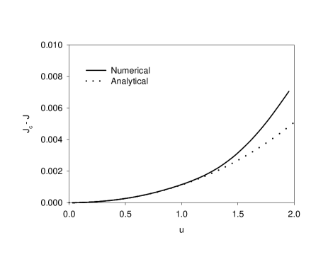
FIG. 7.: $(J_{c}-J)$ for the numerical data (solid line) and for the result of the small-$u$ analysis, Eq. (106) (dashed line).

V Moving Interfaces

At currents other than $J^{*}$, the NS interfaces move with a constant velocity. For such solutions the operator $\partial_{t}$ can be replaced by $-c\partial_{x}$, so that Eqs. (IV B) become

$$-cuf_{x}=f_{xx}-fq^{2}+f-f^{3},$$ (108)

$$u(-cq+\mu)f=2f_{x}q+fq_{x},$$ (109)

$$J=f^{2}q-\mu_{x}.$$ (110)

While the boundary conditions on $f$ and $q$ remain the same, that on the scalar potential becomes $\mu_{\infty}=cq_{\infty}$. Actually, it is more convenient to use instead $\tilde{\mu}=\mu-cq$, which is the gauge-invariant potential in the constant-velocity case.

The superconducting phase invades the normal phase if $J<J^{*}$ and vice versa if $J>J^{*}$. For currents near $J^{*}$, the interface speed is proportional to $(J-J^{*})$. In this linear response regime, one can define a kinetic coefficient (which Likharev [14] refers to as a “viscosity”)

$$\eta=\left({dc\over dJ}\right)^{-1}_{J=J^{*}}.$$ (111)

Figure 8 shows the numerically determined kinetic coefficient as a function of $u$. For large-$u$, we find $\eta\sim u^{3/4}$ for which we provide an argument below.

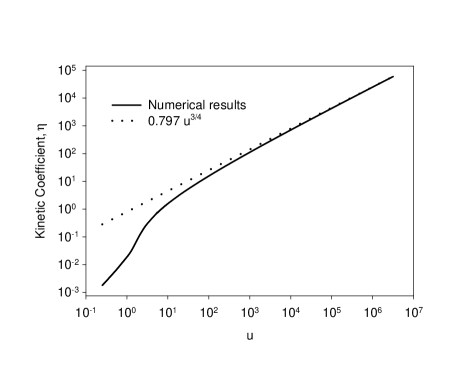
FIG. 8.: A log-log plot of the numerically determined kinetic coefficient as a function of $u$ (the solid line) along with an asymptotic fit of $0.797u^{3/4}$ (the dotted line).

Farther from the stall current, the velocities deviate from this linear behavior, as seen in Fig. 9. The greatest departure occurs in the limits $J\rightarrow 0$ and $J\rightarrow J_{c}$. In fact, Likharev [14] conjectured that the interface speed diverges in both of these limits; we find that it is bounded.

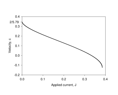
FIG. 9.: The velocity of the front versus the current $J$ for $u=5.79$.

The $J\rightarrow 0$ limit. The moving interface equations, Eqs. (V), simplify in the $J\rightarrow 0$ limit, since that limit implies that both $q\rightarrow 0$ and $\mu\rightarrow 0$, leaving only

$$f_{xx}+ucf_{x}+f-f^{3}=0.$$ (112)

If we replace $uc$ in the above equation by a speed $v$, then we have the steady-state version of Fisher’s equation [31], which is known to have propagating front solutions with $v=2$ [32]. In our case this implies that as $J\rightarrow 0$, $c=2/u$, which is in good agreement with the numerical data shown in Fig. 9.

We can combine the above result with an earlier one to suggest that $\eta\sim u^{3/4}$ as $u\rightarrow\infty$. In the large-$u$ limit, we have information on the following two points: (1) the stalled interface ($J=J^{*}\sim u^{-1/4},c=0$); and (2) the interface in the absence of current ($J=0,c=2/u$). In going from (1) to (2), the changes in current and velocity are $\Delta J\sim u^{-1/4}$ and $\Delta c\sim u^{-1}$. As $u\rightarrow\infty$, both of these changes are small so that $\eta$ might be approximated by

$$\eta\approx{\Delta J\over\Delta c}\sim u^{3/4},$$ (113)

yielding the behavior seen in the numerical data (see Fig. 8 and Table II).

The $J\rightarrow J_{c}$ limit. The numerical work indicates that the velocity is finite as $J\rightarrow J_{c}$; the limiting velocity is shown in Fig. 10 as a function $u$. We can find an analytic bound on this velocity as follows. First, take Eqs. (V), use the gauge-invariant potential $\tilde{\mu}$, and find the constant-velocity analog of Eq. (43). Then substitute the asymptotic forms, Eqs. (IV B), into the resulting equations, leading to

$$\left(cu\lambda_{f}^{-1}+\lambda_{f}^{-2}-2f_{\infty}^{2}\right)f_{1}{\rm e}^{x/\lambda_{f}}=2f_{\infty}q_{\infty}q_{1}{\rm e}^{x/\lambda_{q}},$$ (115)

$$\left(uf_{\infty}^{2}-\lambda_{\mu}^{-2}\right)\tilde{\mu}_{1}{\rm e}^{x/\lambda_{\mu}}=cq_{1}\lambda_{q}^{-2}{\rm e}^{x/\lambda_{q}},$$ (116)

$$2f_{\infty}q_{\infty}f_{1}{\rm e}^{x/\lambda_{f}}+\left(f_{\infty}^{2}-c\lambda_{q}^{-1}\right)q_{1}{\rm e}^{x/\lambda_{q}}$$ (117)

$$\ \ \ \ \ \ \qquad\qquad\qquad-\tilde{\mu}_{1}\lambda_{\mu}^{-1}{\rm e}^{x/\lambda_{\mu}}=0.$$ (118)

Arguments similar to those following Eqs. (IV B) lead one to the conclusion that in this case $\lambda_{f}=\lambda_{q}=\lambda_{\mu}$. The above equations can then be shown to yield the following relation

$$u^{2}c^{2}+\left(2u\lambda^{-1}-2uf_{\infty}^{2}\lambda-u^{2}f_{\infty}^{2}\lambda\right)c$$ (119)

$$+\left[2\left(uf_{\infty}^{2}\lambda^{2}-1\right)\left(3f_{\infty}^{2}-2\right)-uf_{\infty}^{2}+\lambda^{-2}\right]=0,$$ (120)

where we have used $q_{\infty}^{2}=1-f_{\infty}^{2}$. We find the bound by: (1) solving Eq. (119) for $c$; (2) substituting in $f_{\infty}=\sqrt{2/3}$ (which corresponds to $J=J_{c}$); and (3) extremizing that result with respect to the decay length $\lambda$. The small-$u$ limit of the resulting bound is $-\sqrt{2u}/9$, and the large-$u$ limit is $-1/2\sqrt{3}$. The square-root dependence of the velocity in the small-$u$ limit agrees with the data. Now we can consider going from the stall current $(J^{*},c=0)$ to the critical depairing current $(J_{c},c\sim u^{1/2})$ which results in changes $\Delta J\sim u^{2}$ and $\Delta c\sim u^{1/2}$, suggesting that the small-$u$ kinetic coefficient $\eta\sim u^{3/2}$, which is in rough agreement with the numerical data. We have also observed that as a function of $J$ the speed appears to approach its bound via a square root dependence

$$c(J)=A+B(J_{c}-J)^{1/2}$$ (121)

for all $u$.

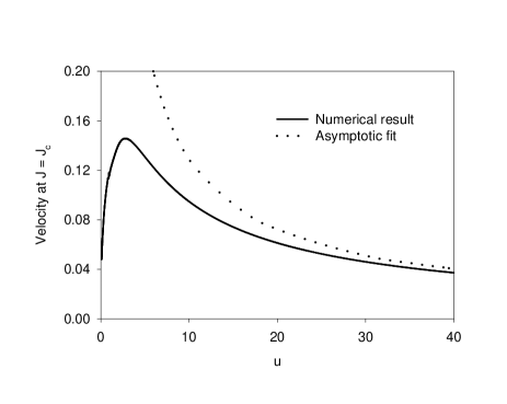
FIG. 10.: The velocity as $J\rightarrow J_{c}$ as a function of $u$. For large $u$, the velocity asymptotically approaches $0.92u^{-0.85}$.

VI Summary and Remarks

In this paper we have studied in detail the nucleation and growth of the superconducting phase in the presence of a current. The finite amplitude critical nuclei grow as the current is increased, with the amplitude eventually saturating as the stall current $J^{*}$ is approached, leading to the formation of interfaces separating the normal and superconducting phases. The stall current can be calculated in the limit of large $u$ using matched asymptotic expansions, demonstrating once again the utility of this technique for problems in inhomogeneous superconductivity. We have also derived an analytic expression for the stall current for small $u$, which we believe to be correct up to exponentially small corrections. Deviations from the stall current cause the interfaces to move, and we have calculated the mobility of these moving interfaces for a wide range of $u$. Finally we have shown that the interface velocity $c=2/u$ as $J\rightarrow 0$ and that $c$ is bounded as $J\rightarrow J_{c}$, in contrast to some conjectures in the literature.

As in the magnetic-field analogy, the issue of stability and dynamics of the current-induced NS interfaces will be more complicated and interesting in the two-dimensional case. Some preliminary work in this direction has been reported by Aranson et al.[17], who find that the current has a stabilizing effect on the NS interface. This can be interpreted as a positive surface tension for the interface, due entirely to nonequilibrium effects. They provide a heuristic derivation of an interesting free-boundary problem for the interfacial dynamics (a variant of the Laplacian growth problem); however, this free-boundary problem is sufficiently complicated that they were unable to solve it to compare with their numerical results. Clearly, further work in this direction would be helpful in understanding the nucleation and growth of the superconducting phase in two-dimensional superconducting films.

A Amplitude of the critical nuclei in the $J\rightarrow 0$ limit

In this appendix we provide a self-consistent calculation of the amplitude of the critical nuclei in the $J\rightarrow 0$ limit. Choosing the gauge appropriate for bumps centered at $x=0$ and combining Eqs. (II) into one equation yields

$$\left[-u\partial_{t}+iuJx+\partial_{x}^{2}+1\right]\psi(x,t)=|\psi(x,t)|^{2}~{}\psi(x,t)$$ (A1)

$$\ \ \ \ \ \ +iu\left[\int_{0}^{x}dy~{}{\rm Im}\left(\psi^{*}(y,t)\partial_{y}\psi(y,t)\right)\right]\psi(x,t).$$ (A2)

The propagator for the linear operator appearing on the left hand side of Eq. (A1) satisfies the condition

$$\left[-u\partial_{t}+iuJx+\partial_{x}^{2}+1\right] G(x,x^{\prime};t-t^{\prime})\Theta(t-t^{\prime})$$ (A3)

$$= -u~{}\delta(x-x^{\prime})\delta(t-t^{\prime})$$ (A4)

and is given by

$$G(x,x^{\prime};\tau)= \left(\frac{u}{4\pi\tau}\right)^{1/2}\exp\left[\frac{\tau}{u}-\frac{J^{2}\tau^{3}}{12u}\right]$$ (A6)

$$\times\exp\left[\frac{iJ\tau(x+x^{\prime})}{2}-\frac{u(x-x^{\prime})^{2}}{4\tau}\right].$$

Ivlev et al. [29, 15] used this linear propagator to evolve perturbations having widths of $O(1)$ and carrying no current. Without the nonlinear terms such perturbations initially grow but ultimately reach a maximum size and then decay away. Ivlev et al. suggested that the amplitudes of the critical nuclei are exponentially small in the $J\rightarrow 0$ limit by asking what sized initial perturbations are of $O(1)$ at their maxima. Their arguments motivated us to use the propagator in a more careful estimate of the amplitude that includes the nonlinear terms as an essential ingredient.

We can convert Eq. (A1) into an integral equation by multiplying both sides of Eq. (A1) (with $x\rightarrow x^{\prime}$ and $t\rightarrow t^{\prime}$) by $G(x,x^{\prime};t-t^{\prime})$ and integrating over all $x^{\prime}$ and integrating $t^{\prime}$ from $0$ to $t$. After some manipulation these steps lead to

$$\psi(x,t) =\int_{0}^{t}dt^{\prime}\int_{-\infty}^{\infty}dx^{\prime}~{}G(x,x^{\prime},t-t^{\prime})$$ (A7)

$$\times \left\{\psi(x^{\prime},t^{\prime})\delta(t-t^{\prime})-\frac{1}{u}|\psi(x^{\prime},t^{\prime})|^{2}~{}\psi(x^{\prime},t^{\prime})\right.$$ (A8)

$$-i \left.\left[\int_{0}^{x^{\prime}}dy~{}{\rm Im}\left(\psi^{*}(y,t^{\prime})\partial_{y}\psi(y,t^{\prime})\right)\right]\psi(x^{\prime},t^{\prime})\right\},$$ (A9)

where $t>0$.

In order to estimate the amplitude of the threshold solutions, we will substitute into Eq. (A7) the following form

$$\psi(x,t)=\psi_{0}\exp\left\{-\frac{uJx^{2}}{4}+ix\right\}.$$ (A10)

Note that this form is stationary and has a fixed Gaussian shape (which is inspired by our WKB approximation, see Eq. (25)) but it has an arbitrary amplitude which we will determine self-consistently.

Let us take the $t\rightarrow\infty$ limit and focus on $x=0$ since our interest is in the amplitude. After substituting Eq. (A10) into Eq. (A7), we can do both integrals for the first term on the right hand side exactly, and it can be seen to decay to zero in the $t\rightarrow\infty$ limit. Next, we perform the $x^{\prime}$ integration of the second term on the right hand side ($II$), which yields

$$II=-\frac{\psi_{0}^{3}}{uJ}\int_{0}^{\infty}\frac{d\tau}{\sqrt{1+3\tau}}\exp\left\{\frac{24\tau^{2}-4\tau^{3}-3\tau^{4}}{12uJ(1+3\tau)}\right\},$$ (A11)

where $\tau=Jt$. We now apply the method of steepest descent to obtain

$$II\approx-\frac{\sqrt{\pi}\psi_{0}^{3}}{\sqrt{2uJ}}\exp\left\{\frac{32}{81~{}uJ}\right\}.$$ (A12)

In the third term on the right hand side ($III$) of Eq. (A7), we make the substitution $y=vx^{\prime}$ and then perform the $x^{\prime}$ integration giving

$$III = \frac{\psi_{0}^{3}}{uJ^{2}}\int_{0}^{\infty}d\tau\int_{0}^{1}dv\frac{(2\tau+\tau^{2})}{\sqrt{[1+\tau(1+2v^{2})]^{3}}}$$ (A14)

$$\times\exp\left\{\frac{24v^{2}\tau^{2}-4\tau^{3}-(1+2v^{2})\tau^{4}}{12uJ[1+(1+2v^{2})\tau]}\right\}.$$

The maximum of the term in the exponential of $III$ occurs at $v=1$ (which is an endpoint). Linearizing about that maximum provides

$$III \approx \frac{\psi_{0}^{3}}{uJ^{2}}\int_{0}^{\infty}\frac{d\tau\tau(2+\tau)}{\sqrt{(1+3\tau)^{3}}}\exp\left\{\frac{24\tau^{2}-4\tau^{3}-3\tau^{4}}{12uJ(1+3\tau)}\right\}$$ (A16)

$$\times\int_{0}^{1}dw\exp\left\{-\frac{\tau^{2}(2+\tau)^{2}w}{uJ(1+3\tau)^{2}}\right\},$$

where $w=1-v$. After the $w$ integration, we apply the method of steepest descent to the $\tau$ integration to obtain

$$III\approx\frac{\sqrt{\pi u}\psi_{0}^{3}}{\sqrt{2J}}\frac{9}{8}\exp\left\{\frac{32}{81~{}uJ}\right\}.$$ (A17)

Putting all of these results back into Eq. (A7) gives

$$\psi_{0}\approx\frac{\sqrt{\pi u}\psi_{0}^{3}}{\sqrt{2J}}\exp\left\{\frac{32}{81~{}uJ}\right\}\left[\frac{9}{8}-\frac{1}{u}\right],$$ (A18)

which provides the expression given in the text, Eq. (27). This calculation clearly runs into trouble when $u<8/9$; however, the numerical coefficients in front of these integrals are sub-leading terms, and they can be varied by adding sub-leading terms to the initial Gaussian guess.

REFERENCES

- [1] Electronic address: ajd2m@virginia.edu
- [2] Electronic address: teb2n@virginia.edu
- [3] Electronic address: dorsey@phys.ufl.edu
- [4] Electronic address: mf1i@virginia.edu
- [5] H. Frahm, S. Ullah, and A. T. Dorsey, Phys. Rev. Lett. 66, 3067 (1991).
- [6] F. Liu, M. Mondello, and N. D. Goldenfeld, Phys. Rev. Lett. 66, 3071 (1991).
- [7] S. J. Di Bartolo and A. T. Dorsey, Phys. Rev. Lett. 77, 4442 (1996).
- [8] A. T. Dorsey, Ann. Phys. 233, 248 (1994).
- [9] J. C. Osborn and A. T. Dorsey, Phys. Rev. B 50, 15 961 (1994). See also C. J. Boulter and J. O. Indekeu, Phys. Rev. B 54, 12 407 (1996).
- [10] S. J. Chapman, Quart. J. Appl. Math. 53, 601 (1995).
- [11] A. B. Pippard, Phil. Mag. 41, 243 (1950).
- [12] S. J. Chapman, IMA J. Appl. Math. 54, 159 (1995).
- [13] R. E. Goldstein, D. P. Jackson, and A. T. Dorsey, Phys. Rev. Lett. 76, 3818 (1996); A. T. Dorsey and R. E. Goldstein, preprint (cond-mat/9704161).
- [14] K. K. Likharev, JETP Lett. 20, 338 (1974).
- [15] B. I. Ivlev and N. B. Kopnin, Sov. Phys. Usp. 27, 206 (1984).
- [16] L. Kramer and A. Baratoff, Phys. Rev. Lett. 38, 518 (1977).
- [17] I. Aranson, B. Ya. Shapiro, and V. Vinokur, Phys. Rev. Lett. 76, 142 (1996).
- [18] A. Schmid, Phys. Kondens. Mater. 5, 302 (1966).
- [19] L. P. Gor’kov and G. M. Eliashberg, Sov. Phys. JETP 27, 328 (1968).
- [20] For a general introduction to the method of matched asymptotic expansions, see C. M. Bender and S. A. Orszag, Advanced Mathematical Methods for Scientists and Engineers (McGraw-Hill, New York 1978); M. van Dyke, Perturbation Methods in Fluid Mechanics (The Parabolic Press, Stanford 1975). For some recent applications to problems in superconductivity, see Refs. [8] and [10], and A. J. Dolgert, S. J. Di Bartolo, and A. T. Dorsey, Phys. Rev. B 53, 5650 (1996).
- [21] J. Pearl, Appl. Phys. Lett. 5, 65 (1964).
- [22] S. J. Chapman, Q. Du, and M. Gunzburger, Z. angew. Math. Phys. 47, 410 (1997).
- [23] We warn the reader that this choice is different than in many applications of the TDGL equations, where the penetration depth is chosen as the length scale. In the thin film limit the penetration depth drops out of the calculation, leaving as the length scale.
- [24] B. I. Ivlev, N. B. Kopnin and L. A. Maslova, Sov. Phys. Solid State 22, 149 (1980).
- [25] L. P. Gor’kov, JETP Lett. 11, 32 (1972).
- [26] I. O. Kulik, Sov. Phys. JETP 32, 318 (1970).
- [27] W. H. Press, B. P. Flannery, S. A. Teukolsky and W. T. Vetterling, Numerical Recipes (Cambridge Univ. Press, New York 1986).
- [28] R. J. Watts-Tobin, Y. Krähenbühl and L. Kramer, J. Low Temp. Phys. 42 459 (1981).
- [29] B. I. Ivlev, N. B. Kopnin and L. A. Maslova, Sov. Phys. JETP 51, 986 (1980).
- [30] J. S. Langer and V. Ambegaokar, Phys. Rev. 164, 498 (1967).
- [31] R. A. Fisher, Ann. Eugen. 7, 355 (1937); A. N. Kolmogorov, I. G. Petrovskii and N. S. Pishunov, Bull. Univ. Moscow, Ser. Int. A 1, 1 (1937).
- [32] D. G. Aronson and H. F. Weinberger, Adv. Math. 30, 33 (1978).