[

A Prototype Model of Stock Exchange

Abstract

A prototype model of stock market is introduced and studied numerically. In this self-organized system, we consider only the interaction among traders without external influences. Agents trade according to their own strategy, to accumulate his assets by speculating on the price’s fluctuations which are produced by themselves. The model reproduced rather realistic price histories whose statistical properties are also similar to those observed in real markets.

]

In the modern market of stocks, currencies, and commodities, trading patterns are becoming more and more global. Market-moving information is being transmitted quickly to all the participants (at least in principle). However, not all the participants interpret the information the same way and react at the same time delay. In fact, every participant has a certain fixed framework facing external events. It is well known that the global market is far from being at equilibrium[1], the collective behavior of the market can occasionally have violent bursts (rallies or crushes) and these violent events follow some empirically well established scaling laws. These are currently the subject of intensive studies [2, 3, 4, 5, 6]. It is not settled yet whether these fluctuations are due to external factors or to the inherent interaction among market’s players.

From a physicist’s point of view, the market is an excellent example of self-organized systems: each agent decides according to his own perception of the events. In the simplest framework, these events consist in the price fluctuations, the only available information. Each participant’s action will in turn influence the price. In a true economy there are external driving factors, such as politics, natural disasters, human psychology etc. Another systematic effect is due to the periodicity of human life (days, weeks, months and years) which also influences the dynamics of prices. From the theoretical side, it is interesting to understand whether the statistical properties of prices depend directly on the external driving factors or whether they are self generated by the system itself.

In the present work, sticking to a physicist’s point of view, we shall address this issue by investigating this system in the absence of external factors. Thus in our market all the participants are speculators: they trade with the sole aim to increase their capital. We shall see that a very rich and complex statistics of price fluctuations emerges from such a closed system of traders which speculate on the price fluctuations they produce themselves. In spite of the simplicity of our model and of the strategies of the single participants, and the outright exclusion of economic external factors, we shall find a market which behaves surprisingly realistically. These results suggest that a stock market can be considered as a self-organized critical system: The system reaches dynamically an equilibrium state characterized by fluctuations of any size, without the need of any parameter fine tuning or external driving.

Let us define our model more precisely. Each player is initially given the same amount of capital in two forms: cash $M_{i,t=0}$ and stock $S_{i,t=0}$. At any time $t$ the capital of player $i$ is given by $C_{i,t}=M_{i,t}+p_{t}S_{i,t}$, where $p_{t}$ is the current price of the stock. There is only one stock in this model, e.g. a foreign currency. All trading consists of switching back and forth between cash and this stock. Each player has a strategy that makes recommendation for buying or selling a certain amount of stock for the next time step. This depends solely on the information available, i.e. the past price history. All the players have equal access to the price history. The actions taken by each player is bounded by his belongings. Player $i$ can invest only a fraction of his stocks which, at any time $t$, is given by his strategy: At time $t$, the general form of the strategy of player $i$ is

$\displaystyle{X}_{i,t}=F_{i}[p_{t},p_{t-1},\ldots]$

where $X_{i,t}S_{i,t}$ is the amount of stock player $i$ decides to buy ($X_{i,t}>0$) or to sell ($X_{i,t}<0$). Our model draws inspiration from Brian Arthur’s model of Bar Attendance [7], where each bar hopper can formulate his own prediction, based on the past observation. This shows that, in a game of interacting strategies, the measure of a strategy’s efficacy can be given only a posteriori. Any strategy is, a priori, as good as any other. Therefore, in our case, initially the strategies are randomly chosen. Then, at each time step, the agent with the smallest capital is eliminated and replaced by one with a new (random) strategy. This refreshing rule keeps the population of the traders dynamic and it is a simple application of Darwinism to economy.

Since, the “space of strategies” is enormous, finding some “local maximum” of the fitness is nearly impossible. Moreover it is unrealistic to assume that the action of player $i$ is independent of his belongings $M_{i,t}$ and $S_{i,t}$.

For these two reasons we i) parametrized the functions $F_{i}$ in terms of indicators $I_{k}\{p\}$ and ii) we introduced a restoring effect which tends to balance the ratio $S_{i,t}/M_{i,t}$ to the current price $p_{t}$. For the indicators we choose moving time averages of combinations of time derivatives of $\log p_{t}$ (e.g. $I_{1}=\langle{\partial_{t}\log p_{t}}\rangle$, $I_{2}=\langle{\partial_{t}^{2}\log p_{t}}\rangle$, $I_{3}=\langle{[\partial_{t}\log p_{t}]^{2}}\rangle$, etc). The time averages were done over a time period of typically $10\sim 100$ time steps[9]. Note that considering time differences of $\log p$ and not of $p_{t}$, makes the indicators, and hence the strategies, depend on relative fluctuations of $p_{t}$ and not on his absolute value. The strategies were then parametrized by $\ell$ numbers $\eta_{i,k}$:

$\displaystyle{X}_{i,t}=f\left(\sum_{k=1}^{\ell}\eta_{i,k}I_{k}\{p\}\right)$

where $f(x)$ is a non-linear function. The nonlinearity of $f(x)$ is introduced to mimic, to some extent, the behavior of agents in a realistic market. Agents indeed sometimes play “contrarian” strategies, i.e. strategies which do not follow the trend. In a rally run, an agent may take advantage of short selling in anticipation of a reverse or crush. Furthermore, $f(x)$ must be less than $1$, since it represents the fraction of one agent’s stock moved in a time step. Note also that large arguments of $x$ occur for example in the presence of wild fluctuations of $p_{t}$. The behavior of traders becomes in these cases very cautious, which implies $f(x)\ll 1$ for $x$ large. To imitate these behaviour we took $f(x)=x/[1+(x/2)^{4}]$.

The amount of stock $\Delta S_{i,t}$ agent $i$ decides to sell ($\Delta S_{i,t}<0$) or to buy ($\Delta S_{i,t}>0$) is given by

$$\Delta S_{i,t}={X}_{i,t}S_{i,t}+\frac{\gamma_{i}M_{i,t}-p_{t}S_{i,t}}{2\tau_{i}}.$$ (1)

Here the first term is pure speculation, whereas the second introduces a dependence on $M_{i,t}$ and $S_{i,t}$ in the action of player $i$. In order to motivate this term, consider the event where, for some reason the price remains constant $p_{t}=p_{0}$ for a long period. A realistic behavior of the agents in such a situation would be that to ri-equilibrate their portfolio at their chosen level $S_{i,t}/M_{i,t}=p_{0}/\gamma_{i}$. These operations at constant price do not change the capitals $C_{i,t}$. On the contrary, having his assets equilibrated at the actual price, a player is in the most favorable situation to face possible future price fluctuations of either sign. The second term in eq. (1) reproduces this behavior. Indeed if the price is constant, all indicators $I_{k}$ vanish and so do all speculation terms $X_{i,t}$. In the absence of the first term, the second equilibrates the ratio $S_{i,t}/M_{i,t}$ to a value $p/\gamma_{i}$ within a time of order $\tau_{i}$.

In summary the strategy of each player is parameterized by $\ell+2$ numbers: $\eta_{i,1},\ldots,\eta_{i,\ell},\gamma_{i}$ and $\tau_{i}$. Once the price $p_{t}$ is fixed, it is communicated to the players who can decide their actions $\Delta S_{i,t}$. The transactions then take place at this price $p_{t}$. Let us define the total demand and offer of stocks at time $t$

$\displaystyle D_{t}=\sum_{i:\Delta S_{i,t}>0}\Delta S_{i,t}\qquad O_{t}=-\sum_{i:\Delta S_{i,t}<0}\Delta S_{i,t}.$

When the demand is larger than the offer, the players willing to buy $\Delta S_{i,t}>0$ stocks will in fact be able to buy only the available amount $\bar{\Delta}S_{i,t}=\Delta S_{i,t}O_{t}/D_{t}$, whereas players who sell will sell all their $-\Delta S_{i,t}$ stocks ($\bar{\Delta}S_{i,t}=\Delta S_{i,t}$). The reverse situation will clearly apply if $D_{t}<O_{t}$. Our model also includes a finite cost $\pi\Delta S_{i_{t}}$ on the buyers ($\pi\sim 10^{-3}$) and random fluctuations $\epsilon_{i,t}M_{i,t}$ in the cash of each agent ($\epsilon_{i,t}$ is a random variable uniformly distributed in $[-\epsilon,\epsilon]$) which, loosely speaking, represents the “heat bath” fluctuations due to all the other actions of player $i$. These rules are summarized in the following equation:

$$\left.\begin{array}[]{l}S_{i,t+1}=S_{i,t}+\bar{\Delta}S_{i,t}\\ M_{i,t+1}=[1+\epsilon_{i,t}][M_{i,t}-p_{t}(1+\pi)\bar{\Delta}S_{i,t}]\end{array}\right\} \hbox{if $\bar{\Delta}S_{i,t}>0$},$$

$$\left.\begin{array}[]{l}S_{i,t+1}=S_{i,t}+\bar{\Delta}S_{i,t}\\ M_{i,t+1}=[1+\epsilon_{i,t}][M_{i,t}-p_{t}\bar{\Delta}S_{i,t}]\end{array}\right\} \hbox{if $\bar{\Delta}S_{i,t}<0$}.$$

FIG. 1.: Price history for a system of $1000$ agents. The parameters are $\epsilon=0.01$ and $\pi=10^{-3}$. In the lower part the zoom of the area in the upper rectangle.

Next a new price $p_{t+1}$ is determined. This is done implementing the law of demand and offer in the form

$$p_{t+1}=p_{t}\frac{\langle{D_{t}}\rangle}{\langle{O_{t}}\rangle}$$ (4)

where the averages are, as before time averages. Note that the price raises when there is a large demand and falls when the offer is large. Also note that this form of the law of demand and offer is dimensionally correct.

Our numerical simulations are quite encouraging. Despite the simplicity and the arbitrariness of the strategies, an extremely rich price history is created. A sample of $p_{t}$ is shown in fig. 1. This shows fluctuations of all sizes. Depending on the parameters, on long runs, also some crushes occasionally occur, with almost no sign of its coming. These crushes arise only as a result of collective trading activity. Apart from a simple “smoothing” [9] which becomes more efficient in the presence of wild fluctuations, our model does not implement the many corrections which are taken in similar cases by central authorities in a real market.

The signal is similar to that of stock prices or foreign currencies. This impression is confirmed analyzing the temporal signal. Recently quite a few empirical studies have been carried out for the statistics of economics time series, notably the Standard & Poor’s 500 index[3], and high frequency foreign exchange data[5, 6].

When comparing our statistical data, the definition of time becomes a matter of concern. In our model the time flows uniformly and the number of agents are fixed. In a real economy there are periods of inactivity, when the market closes, and the number of active agents varies with time. This leads to systematic periodic variations in the signal $p_{t}$ so that its fluctuations $x=p_{t+\tau}-p_{t}$ can no longer be considered as a stationary variable. This issue was discussed at length in ref. [6] where a time transformation which eliminates these systematic effects was introduced. Our model clearly does not contain these systematic effects and therefore better compares with real economic data in the transformed time[6].

FIG. 2.: Probability $F(x=0,\tau)$ of price returns (i.e. $x=0\Rightarrow p_{t+\tau}=p_{t}$) vs $\tau$. The parameters are the same as in fig. 1.

Following refs. [3, 5, 6], let us define the histogram $F(x,\tau)$ of price variations $x=p_{t+\tau}-p_{t}$. Figure 2 shows that the scaling behavior of the the price “returns” $F(0,\tau)$ is very similar to that observed in a real economy, it behaves like $\tau^{-H}$ with an exponent $H\simeq 0.62$.

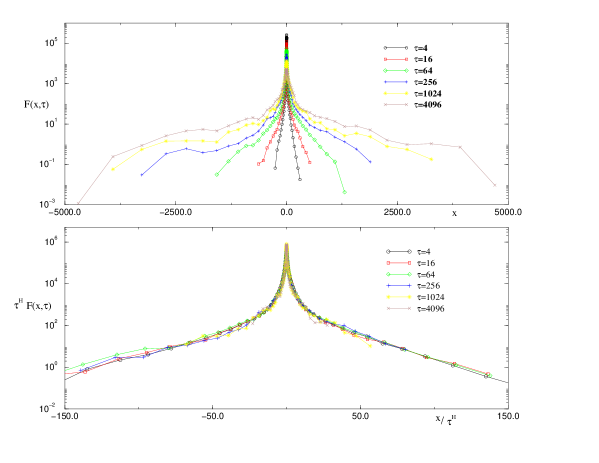
FIG. 3.: Upper part: histogram of price variations for several values of $\tau$. Lower part: collapse plot of the previous data with $H=0.62$. The parameters are the same as in fig. 1.

The full distribution $F(x,\tau)$ is shown in figure 3 for several values of $\tau$. These distributions satisfy the scaling hypothesis

$$F(x,\tau)=\tau^{-H}F\left(x\tau^{-H},1\right)=\tau^{H}g\left(x\tau^{-H}\right),$$ (5)

with an exponent $H=0.62$, as shown in the lower part of fig. 3. This is very similar to the behavior of prices in a real economy. The tails of the distributions have a power law character $F(x,\tau)\sim x^{-\alpha}$ with exponent $\alpha$ close to $2$. This differs from what is seen in real economic data where either the exponent is larger ($\approx 4.5$ [6]) or the decay is more rapid [3]. We believe that this is due to the fact that the tail of the distribution describes extreme events. Under extreme events, in a real economy, the rules of the game change drastically. On the contrary in our model the rules are always the same no matter what fluctuations $p_{t}$ may suffer.

In the stationary state, one can classify the traders according to their wealth. Zipf [8] has observed that the distribution of economic power among individuals of a society follow a well defined power law, hence the name Zipf’s law. In our artificial society we plot the assets distribution in the Zipf’s fashion where the capital $C(n)$ of the $n^{\rm th}$ richer person is plotted against the order $n$. Figure 4 shows this law (note that the plot refers to one single snapshot of a system of $1000$ agents). Our exponent $\approx-1.2$ is not too far from Zipf’s value for the distribution of cooperation assets[8].

With respect to the robustness of the results, we found that particular care has to be paid in order to avoid crushes and singularities in the market. For all choices of parameters yielding a stable behavior, we found similar results. But, for example, including “copying”,i.e. the possibility for a poor to copy the strategy of a richer, changes the exponent $H$ from $0.62$ to $0.5$. Interestingly, in the model with copying, we also detected a multiscaling behavior of the same form of the one discussed in [5]. A weak multiscaling, or no multiscaling at all, was instead found in the dynamics without copying.

FIG. 4.: The capitals $C(n)$ owned by each player in order of richness. The parameters are the same as in fig. 1.

In conclusion we find realistic behavior in a simple model for a stock market without external driving. The players trade in an non-ending fight against each other to survive. Such a dynamic system produce a non trivial time series behind, which records all the infighting and ingenuity of the players trying to out-guess others. Simple signal forms are expected to be excluded since they are too easy to anticipate. The result is a signal with all the surprises of all sizes (for the traders as well as for us!). We have purposely excluded any real information input, our results nevertheless show close resemblance to real markets. This suggests that the statistics we observe in real markets is mainly due to the interaction among “speculators” trading on technical grounds, regardless of economic fundamentals. Indeed it is known that in Foreign exchange markets the trades by speculators far outnumbers the trades due to real commercial needs.

It is clear that by no means one can conclude that our model captures all the relevant aspects of a real market. As already said it misses the effects of external drive. More importantly, it does not contain adaptive dynamics of the player’s strategies. Further studies should answer the question: what are the essential elements in a model that will reproduce realistic results? In this perspective our model can be considered as a first step in this challenging direction.

GC acknowledges the University of Fribourg for the kind hospitality, Anna B. and Domenico C. for useful hints. We are also grateful to S. Galluccio for helpful discussions.

REFERENCES

- [1] P. W. Anderson, K. J. Arrow and D. Pines, The Economy as an Evolving Complex System, Addison Wesley (1988).
- [2] B.B. Mandelbrot, J. of Business, 36, 394 (1963); B.B. Mandelbrot, The Journal of Business of the University of Chicago, 39, 242 (1966); B.B. Mandelbrot, The Journal of Business of the University of Chicago, 40, 393 (1967).
- [3] R.N. Mantegna, Physica A, 179, 232 (1991); R.N. Mantegna and H.E. Stanley, Nature, 376, 46 (1995).
- [4] A. Arneodo, J.P. Bouchaud, R. Cont, J.F. Muzy, M. Potters and D. Sornette, Comment on “Turbulent Cascades in foreign Exchange Markets”, submitted to Nature; Cond-mat. preprint 9607120.
- [5] S. Ghasghaie, W. Breymann, J. Peinke, P. Talkner and Y. Dodge, Nature 381, 767 (1996).
- [6] S. Galluccio, G. Caldarelli, M. Marsili and Y.-C. Zhang, to appear in Physica A.
- [7] W. B. Arthur, On learning and adaptation in the economy, Santa Fe Institute working paper, 92-07-038 (1992).
- [8] G. K. Zipf, Human Behavior and the Principle of Least Action, Addison-Wesley (1949). Note that Zipf’s law is much more general, it concerns all human behaviors, notably linguistics.
- [9] Time averages were computed run time using an exponential kernel: . The value of was also determined run time according to the volatility: During periods with large fluctuations of the time average was extended (i.e. was increases towards ) to a longer period.