Doped Antiferromagnets in High Dimension

Abstract

The ground-state properties of the $t-J$ model on a $d$-dimensional hypercubic lattice are examined in the limit of large $d$. It is found that the undoped system is an ordered antiferromagnet, and that the doped system phase separates into a hole-free antiferromagnetic phase and a hole-rich phase. The latter is electron free if $J>4t$ and is weakly metallic (and typically superconducting) if $J<4t$. The resulting phase diagram is qualitatively similar to the one previously derived for $d=2$ by a combination of analytic and numerical methods. Domain wall (or stripe) phases form in the presence of weak Coulomb interactions, with periodicity determined by the hole concentration and the relative strength of the exchange and Coulomb interactions. These phases reflect the properties of the hole-rich phase in the absence of Coulomb interactions, and, depending on the value of $J/t$, may be either insulating or metallic (i.e. an “electron smectic”).

]

In this paper, the zero-temperature properties of the $t-J$ model of a doped antiferromagnet on a $d$-dimensional hypercubic lattice are evaluated using a systematic expansion in powers of $1/d$. For each property of interest the leading behavior in the large $d$ limit is computed, and in some cases, just to prove how tough we are, corrections up to order $1/d^{5}$ are obtained. These results are obtained by breaking the full Hamiltonian into an unperturbed piece, $H_{0}$, and a perturbation, $H_{1}$, and then reorganizing conventional perturbation theory in powers of $H_{1}$ into a $1/d$ expansion. Of course the partition of the Hamiltonian may be chosen for calculational convenience, since it does not affect the results. The convergence of this expansion will not be addressed, although we believe it to be only asymptotic.

Our procedure differs from the extensive recent work on the related problem of the Hubbard and Falicov-Kimball models in large dimension[1] in the way the large dimension limit is taken. First of all, we do not assume that the ratio $J/t$ of the exchange integral $J$ and the hopping amplitude $t$ is parametrically small as $d\rightarrow\infty$. The previous studies assumed that $t$ is proportional to $1/\sqrt{d}$ so that, when $J$ is expressed in terms of the onsite interaction $U$, it follows that $J/t=4t/U\sim 1/\sqrt{d}$. (The phase diagram will be studied for parametrically small values of $J/t$ in Sec. VIII, but our results are less complete in this case, because of the difficulty of controlling perturbation theory in this limit.) Secondly, the hypercubic lattice is bipartite, i.e. it can be broken into two sublattices, which we label “black” and “red”, such that the Hamiltonian has interactions only between sites on different sublattices. This favors the classical Néel state, which has a uniaxial magnetization with opposite sign on the two sublattices. By contrast, earlier studies, which were primarily concerned with the Mott transition and possible non-Fermi liquid states of the Hubbard model, assumed a non-bipartite lattice which frustrates the Néel state. For both reasons, this previous work does not shed much light on the behavior of doped antiferromagnets. A notable exception is the work of van Dongen[2] on the small $U$ limit of the Hubbard model on a hypercubic lattice which found, as we do, that the weakly-doped antiferromagnetic phase is unstable to phase separation, even if the parameters are scaled as $J^{eff}/t=4t/U\sim 1/\sqrt{d}$.

Throughout this paper, units are chosen such that the lattice constant, $\hbar$, and Boltzmann’s constant are all equal to one.

I Summary of Results

A Results in Large Dimension

Our principal result is the global zero-temperature phase diagram as a function of $J/t$ and hole concentration $x$, in the limit of large $d$, as shown in Fig. 1. It is immediately clear that in most of the phase diagram, the undoped (ordered) antiferromagnetic phase coexists with a hole-rich phase. For $J/t>4$, the hole-rich phase is electron free; otherwise it contains an exponentially small but non-vanishing concentration of electrons. In the intermediate coupling regime, $2<J/t<4$, the residual attraction ( $J$ ) between electrons is great enough to overcome the hard-core repulsion, and leads to a BCS instability of the dilute metal, producing an s-wave superconducting state at exponentially low energy scales. At smaller values of $J/t$, the net interaction between electrons is repulsive. This implies that the system either remains metallic down to zero temperature or exhibits higher-angular-momentum pairing [3] via the Kohn-Luttinger mechanism.[4]

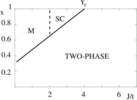
FIG. 1.: Phase diagram of the $t-J$ model in the limit $d\rightarrow\infty$: Here $x$ is the hole concentration ($1-x$ is the electron concentration). The phase boundary is given by Eq. (86), artificially setting $d=2$. “Two-phase” labels the two-phase region, where a uniform density phase is thermodynamically unstable, “SC” labels a region of $s-$ wave superconductivity, and “M” labels a region of metallic behavior with repulsive interactions, which presumably has an ultra-low temperature superconducting instability due to the Kohn-Luttinger effect.[4]

A peculiarity of the phase diagram in Fig. 1 is that the boundary of the two-phase region intersects the $J/t=0$ axis at a non-zero value of $x$. This is not likely to be correct in any finite dimension. For small $x$ and large but finite dimension, we expect that in the limit $J/t\rightarrow 0$, the ground state is a ferromagnetic Fermi liquid, and hence the model does not phase separate. In Section VIII, we discuss the behavior of the model for $J/t$ parametrically small, $J/t\sim 1/\sqrt{d}$. Here the $1/d$ expansion is slightly more difficult to control, so our results, summarized in Fig. 2, are incomplete. The resulting conjectural phase diagram for large but finite $d$ embodies all the insights gained from studying the $d\rightarrow\infty$ limit, but corrects the unphysical features of the phase diagram in Fig. 1.

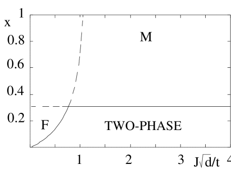
FIG. 2.: Conjectured Phase diagram of the $t-J$ model for large but finite $d$: This figure should be viewed as a blowup of the small $J/t$ portion of Figure 1. The horizontal line represents the small $J/t$ extension of the phase boundary in Fig. 1; in fact, in large $d$, this line would be exponentially close to the top of the figure, but we have drawn it, as in Fig. 1, at a position obtained by setting $d=2$ in the large $d$ expression. The boundary of the fully polarized ferromagnetic metallic phase (labelled “F”) is drawn in accord with the large $d$ expression in Eq. (118. There might be other, lower energy phases, (e.g. high-density stripe phases) that could occur below these two phase boundaries, in the region marked “two-phase”, especially close to the point of intersection.

We have also studied the behavior of one or two doped holes and the character of charged domain walls in the antiferromagnet. It will be seen that the latter are stablilized by a long-range Coulomb interaction. These studies bring out an important characteristic of our large-$d$ expansion. Whenever a hole moves in the antiferromagnetic background, it may break a number of bonds of order $d$ at each hop. Consequently, for such processes, the physics is exchange dominated for large-$d$ and it amounts to an expansion in powers of $t/J$. This is true of the motion of one or two holes and of domain wall fluctuations in which holes hop into the environment. However the questions of phase separation, domain wall phase equilibrium, and superconductivity at low electron concentration are not subject to this limitation.

The ensuing discussion will be organized by order of increasing hole concentration.

To leading order in $1/d$ the states of minimum energy of a single hole lie precisely on the magnetic Brillouin zone which also is the Fermi surface of the noninteracting system with a half-filled band. The massive degeneracy of these low energy hole states is lifted by terms of ${\cal O}(1/d^{4})$, and it is found that the absolute minimum occurs at $\vec{k}=(\pi/2)<1,1,1,...>$ together with points related by the point-group symmetry. Moreover, as deduced previously by Trugman[6] in studies of two holes in a two-dimensional antiferromagnet, we find that propagation of pairs of holes is no less frustrated than is the propagation of a single hole, because of a subtle effect of Fermi statistics. There is, however, an effective attraction $\sim 1/d$ between two holes due to the fact that two nearest-neighbor holes break one less antiferromagnetic bond than two far-separated holes; this attraction always leads to a two-hole bound state.

An interesting metastable state is a charged magnetic domain wall (i.e. a $d-1$ dimensional hypersurface with finite hole concentration and suppressed magnetic order). We have found that the most stable domain wall has an electron density which is, to leading order in $1/d$, equal to that of the hole-rich phase which can exist in equilibrium with the antiferromagnet. Thus domain walls can be viewed as a form of local phase separation. Also the domain wall configuration with the lowest surface tension (i.e. energy per unit hyperarea of wall) is the “vertical” site-centered $\pi$ (antiphase) discommensuration in the antiferromagnetic order; i.e. it is parallel to a single nearest-neighbor vector and odd under reflection through a site-centered vertical hyperplane.

We have considered the effect of weak, long-range Coulomb interactions as a perturbation. While this study is not exhaustive, we conclude that, for a substantial range of parameters, the ground state consists of a periodically-ordered array of optimal domain walls of the sort described above, especially when $x$ is small but not too small. In this range of $x$, the ground state is insulating for $J/t>4$, and metallic for $J/t<4$. The latter phase is an “electron-smectic” [7] which exhibits crystalline order in one direction and liquid-like behavior in the transverse ($d-1$) directions. The liquid features are associated primarily with the motion of electrons along the domain wall, and they may be metallic or condensed into a superconducting state.

We have argued previously that the competition between a local tendency to phase separation in a doped antiferromagnet and the long-range Coulomb repulsion between holes produces a large variety of intermediate scale structures, including arrays of domain walls, which are significant features of doped antiferromagnets that we have called “frustrated phase separation” [8, 9]. However, these phenomena have not previously been derived from a microscopic magnetic model.[5] It is particularly striking that, in the appropriate range of parameters, charge and spin density wave order coexist with metallic, and even superconducting behavior.

B How Large Are $d=2$ and $d=3$?

Large $d$ is, of course, only of academic interest; we are interested in the physical dimensions, $d=1$, 2, and 3. The properties of the one-dimensional electron gas (1DEG) are well understood[10] by now, and exhibit behavior that is quite dimension specific. Moreover, for most of the conceivable ordered states, the lower critical dimension for long range order at zero temperature is one, so the 1DEG is not likely to be well understood in terms of adiabatic continuity from large dimension. However, long range order at zero temperature is quite robust in both two and three dimensions, so there is every reason to expect that a $1/d$ expansion will capture the essential physics of many of the zero-temperature thermodynamic states.

To test this conjecture, we would like to make both qualitative and quantitative comparisons between the results of the large $d$ theory and any available exact, or well-controlled numerical or analytic results in two and three dimensions. Table 1 gives a quantitative comparison between the $1/d$ expansion and well-established numerical results for the undoped system, i.e. for the spin-1/2 Heisenberg antiferromagnet. It can be seen that the ground-state energy can be obtained from the low-order expansion in powers of $1/d$ to $0.6\%$ accuracy or better. By carrying the series to higher order, and possibly doing a Padé analysis of the series much improved accuracy for all physical quantities could be expected. In Sec. XI comparison will be made between numerical results and the results of perturbation theory about the Ising limit (Table 2).

	$E_{AF}(2)$	$m(2)$	$E_{AF}(3)$	$m(3)$	$E_{2-leg}(2)$
$d^{0}$	-0.5	0.5	-0.75	0.5	-0.25
$d^{-1}$	-0.625	0.4375	-0.875	0.4583	-0.5
$d^{-2}$	-0.6563	0.4063	-0.8958	0.4444	-0.5625
$d^{-3}$	-0.6631	0.3948	-0.8989	0.4410	-0.5664
$d^{-4}$	-0.6647	0.3903	-0.8993	0.4402	-0.5713
Exact	-0.669	0.307	-	-	-0.5780[12]
Upper	-0.5	-	-0.75	-	-0.375
Lower	-0.75	-	-1.0	-	-0.625

Table 1: Comparison of the results of exact numerical studies[11] (the row labeled “exact”) on the two-dimensional spin-1/2 Heisenberg antiferromagnet with the perturbative results in powers of $1/d$ derived in the present paper. (We have been unable to find corresponding “exact” three dimensional results.) The dimension is indicated by the arguments of the computed quantities. The rows labeled “Upper” and “Lower” give the rigorous upper and lower bounds on the energies obtained in the text. The approximate results are obtained by setting $y\equiv J_{\perp}/J_{z}=1$, $V=0$, and $d=2$ or $3$ in the series expansion, evaluated to the stated order. All energies are measured in units of $J/d$, and the magnetization $m$ is quoted in units in which $g\mu_{B}=1$, where $\mu_{B}$ is the Bohr magneton.

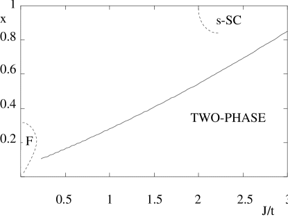
FIG. 3.: Zero Temperature Phase Diagram of the two dimensional $t-J$ model, deduced from numerical studies of finite size systems with up to 60 electrons, as well as from various analytic results. This figure is abstracted from Hellberg and Manousakis.[14]

Qualitative comparisons can be made with the phase diagram of the two dimensional $t-J$ model which has been deduced from combined analytic and numerical[13, 14] studies. Figure 3, abstracted from the work of Hellberg and Manousakis[14] shows the phase diagram deduced from numerical studies of systems with up to 60 electrons. As in large $d$, there is no thermodynamically stable zero-temperature phase with dilute holes for any $J/t$. Indeed, aside from the behavior of the boundary of the two-phase region at very small $J/t$, the phase diagrams in Figs. 1 and 3 are similar. As suggested above, when the pathologies of the formal $d\rightarrow\infty$ limit are removed by taking into account the new processes that become important at parametetrically small values of $J/t\sim d^{-1/2}$, one obtains for large but finite $d$ the phase diagram shown in Figure 2, which is topologically equivalent to Figure 3. (Of course, in $d=2$, parametrically small values of $J/t$ are not all that small, so there is no reason to expect quantitative agreement with the large $d$ results. The critical value of $J/t=Y_{c}$ at which the phase-coexistence line deviates from $x=1$ is[14] $Y_{c}=3.4367$ in $d=2$, and is rather well approximated by the value $Y_{c}\rightarrow 4$ as $d\rightarrow\infty$. However, the slope of the phase coexistence line in $d=2$ is much steeper than would be deduced from the large $d$ theory.) Similar detailed information on the three dimensional $t-J$ model is not available at this time, although arguments presented hitherto [8], [13] suggest that the phase diagram is qualitatively similar to that in $d=2$, consistent with the expectations from the $1/d$ expansion.

Our calculation of the spectrum of one hole in an antiferromagnet may be compared to the numerical calculations of Dagotto et al. [15] on $d=2$ systems with 16$\times$16 sites and $J/t=0.4$. They found that the one-hole spectrum is well represented by the two-dimensional version of the expression in Eq. (63), confirming the qualitative accuracy of the large $d$ expression. However the values of the parameters obtained to leading order in $1/d$ are quantitatively quite far from the exact results, and this discrepancy is made worse by the inclusion of higher order terms. This is not unexpected in view of the fact that large $d$ drives the motion of a single hole into the exchange-dominated limit. In particular, it is clear from Eq. (61) that the large-$d$ expansion gives a negative value for the bandwidth $W$ in $d=2$, unless $J>0.93t$. Thus it is essential to compare the large-$d$ expansion to numerical results at large $J/t$. Specifically, from Eq. (60) with $y=1$, the bandwidth for $d=2$ is given by $dW/t=2.125t/J-1.83(t/J)^{3}$. It would be interesting to compare this result with numerical calculations for large $J/t$ extrapolated to the thermodynamic limit. Martinez and Horsch[16] have found that an approximate treatment of the motion of a single hole gives $dW/t=2t/J$ for large $J/t$, which agrees very well with our large-$d$ result. Via a variational calculation, Bonisegni and Manousakis[17] find $dW/t=0.59\pm 0.15$ in the thermodynamic limit for $d=2$ and $J/t=5$, while Eq. (60) gives 0.41.

Finally, we can extrapolate to two dimensions the character of the ordered arrays of charged domain walls at low doping concentration and weak Coulomb interaction. Domain walls in two dimensions are one-dimensional (lines) and such ordered arrays are known as “stripe phases”. Directly extrapolating the optimal large dimensional domain-wall structures to $d=2$, we would expect the stripes to be site-centered, vertical, antiphase domain walls in the antiferromagnetic order, and to be metallic (and possibly superconducting) for $J/t<Y_{c}$ and insulating for $J/t>Y_{c}$. In particular, if we extrapolate the leading order expression for the electron density in the hole-rich phase, Eq. (87), to $d=2$, and then evaluate it for $t\gg J$, we find that such stripes should have approximately 0.31 doped holes per site along the stripe, and are thus metallic. Transverse to the stripe direction, such a phase is a generalized charge and spin density wave state, in which the period of the charge density wave is half that of the spin density wave.[19] However, because of the electronic motion along the stripe, this phase is actually an electron smectic. [7] Unfortunately, there are no detailed microscopic two dimensional calculations to compare with these results, so we compare them with experiments on doped antiferromagnets.[20]

C Rigorous Results

In addition to our perturbative results in powers of $1/d$, we have obtained rigorous upper and lower bounds on the ground-state energy of the undoped system. These bounds, which are also quoted in Table 1, are shown to converge in the limit $d\rightarrow\infty$.

D Relation to Experimental Results on Doped Antiferromagnets in Quasi-Two and Three Dimensions

By now there are many examples of antiferromagnetic insulators that can be chemically doped. One prominent feature of these materials is the occurrence of high temperature superconductivity, a phenomenon for which the present results provide little direct insight [21]. However various spin and charge ordered states, as well as “nearly ordered” fluctuating versions of such structures, have been observed in these systems [23, 25] by direct structural probes, especially neutron scattering. Two concrete, and well studied examples of this are the quasi two-dimensional perovskites La_2-xSr_xNiO₄ and La_1.6-xNd_xSr_xCuO₄, in both of which the doped hole concentration is equal to the Sr concentration $x$. The undoped parent compounds (with $x=0$) are antiferromagnetic insulators with spin $S=1$ for the nickelates and $S=1/2$ for the cuprates. In both cases, upon doping, the system forms[24, 25] a “stripe” phase, in which the doped holes are concentrated in antiphase domain walls in the antiferromagnetic order. At present it is not known whether the domain walls are site or bond centered in general. (At higher doping concentration in the nickelates, there is strong evidence that both types of domain wall coexist due to interactions between the walls [26].) However, there is a crucial difference between the domain walls in the two materials: In the nickelates, there is one doped hole per site along the domain walls, and the doped system is, correspondingly, insulating. In the cuprate, the hole concentration along the domain wall is roughly one doped hole per two sites along the domain wall, and the system is correspondingly metallic, and even superconducting, despite the presence of almost static charge and spin density wave order. (This latter behavior is very suggestive evidence of an electron-smectic phase.[7]) In addition, the domain walls are diagonal in the nickelates[24] and vertical in the cuprates.[25, 27]

We feel that the occurrence of charged stripes in lightly-doped antiferromagnets, the fact that these stripes are antiphase domain walls in the antiferromagnetic order, and that they can be metallic or insulating, depending on the ratio of $J/t$, are physically robust features of the large $d$ theory which we expect to apply mutatis mutandis in $d=2$. However, the preference for vertical versus diagonal stripes, and site-centered versus bond-centered stripes is likely to depend on microscopic details, even in large dimensions. Of more profound importance is the fact that, while in large dimensions the charged domain walls always crystallize at low temperature into an ordered density wave, in low dimensions, especially in two dimensions, there is the very real possibility that the domain walls will be quantum disordered.[22, 28, 29, 7] In such a melted state, which might be either fully disordered (isotropic) or still retain orientational order (“electron nematic”), the sort of charge and spin-ordered states that are characteristic of the large $d$ theory occur as local correlations in the fluctuation spectrum; a microscopic electronic theory of such quantum disordered states is not available at present.

II The Model

The model we consider is the straightforward generalization of the usual $t-J$ model (or $t-J-V$ model[31]):

$$H= \frac{1}{d}\sum_{<i,j>}\left\{J\vec{S}_{i}\cdot\vec{S}_{j}+Vn_{i}n_{j}\right\}$$ (1)

$$- \frac{t}{d}\sum_{<i,j>,\sigma}\left\{c^{\dagger}_{i,\sigma}c_{j,\sigma}+{\rm H.c.}\right\}$$ (2)

where $\vec{S}_{i}=\sum_{\sigma,\sigma^{\prime}}c^{\dagger}_{i,\sigma}\vec{\sigma}_{\sigma,\sigma^{\prime}}c_{i,\sigma^{\prime}}$ is the spin of the electron on site $i$, $n_{i}=\sum_{\sigma}c^{\dagger}_{i,\sigma}c_{i,\sigma}$ is the number of an electron on site $i$, $c^{\dagger}_{i,\sigma}$ creates an electron with $z$-component of spin equal to $\sigma=\pm 1/2$, $\vec{\sigma}$ are the Pauli matrices, there is a constraint of no double-occupancy of any site,

$$n_{i}=0,1,$$ (3)

and $<i,j>$ signifies nearest-neighbor sites on the $d$-dimensional hypercubic lattice. In comparing results of different calculations, it is important to note that there is more than one definition of the $t-J$ model. Most commonly,[13, 14] “the $t-J$ model” is defined as in Eq. (2) with $V=-J/4$, but without the prefactor of $1/d$. Where it can be done readily, we will quote results for arbitary $V$, but where this leads to complications, we will, for simplicity, analyze only the canonical case $V=-J/4$. The additional factor of $1/d$ is included so that the ground-state energy density remains finite in the $d\rightarrow\infty$ limit; thus, in making a comparison with previous results on the $d=2$ $t-J$ model, all energies computed here should be multiplied by $d=2$.

III The undoped antiferromagnet

The undoped system has one electron per site so that the electron hopping term ($t$) has no effect, and the system is manifestly insulating; the only remaining degrees of freedom are described by a spin 1/2 Heisenberg antiferromagnet with exchange coupling $J$.

A Rigorous Bounds

It is possible to obtain upper and lower bounds on the ground-state energy of the spin-1/2 Heisenberg model which approach each other in the large $d$ limit. An upper bound is obtained by calculating the variational energy of the “Néel” state, which has alternating up and down spins on alternate sites, and gives a ground-state energy per site of $E_{Neel}=-J/4+V$.

A lower bound for the ground-state energy can be obtained[30] as follows: We express the full Hamiltonian as a sum of pieces,

$$H=\sum_{j=black}H_{j}$$ (4)

where the sum is over all sites on the black sublattice and $H_{j}$ is the exchange interactions between site $j$ and its nearest neighbors (which are necessarily on the red sublattice). The Hamiltonians $H_{j}$ are readily diagonalized, but not simultaneously since they do not commute with each other. Nonetheless, the sum of the ground state energies of $H_{j}$ gives the lower bound $E_{lower}=-(1+d^{-1})J/4+V$ for the ground-state energy per site.

These results, combined, prove that the ground-state energy per site, $E_{AF}$, of the Heisenberg model approaches that of the classical Néel state in the limit of infinite dimension,

$$-(J/4)[1+1/d]\leq E_{AF}-V\leq-(J/4).$$ (5)

B Perturbative expression for the ground-state energy and sublattice magnetization

We now embark on the derivation of results in a systematic expansion in powers of $1/d$. For this purpose, we will consider the Heisenberg model as the isotropic limit of a Heisenberg-Ising model. To begin with, we use Rayleigh-Schrödinger perturbation theory to evaluate the properties of interest in powers of the $XY$ coupling, and then reorganize this perturbation theory in powers of $1/d$. Thus, we take as our unperturbed Hamiltonian the Ising piece of the interaction,

$$H_{0}=\frac{1}{d}\sum_{<i,j>}\big{[}J_{z}S_{i}^{z}S_{j}^{z}+Vn_{i}n_{j}\big{]},$$ (6)

and treat the $XY$ piece,

$$H_{1}=\frac{J_{\perp}}{d}\sum_{<i,j>}[S_{i}^{x}S_{j}^{x}+S_{i}^{y}S_{j}^{y}],$$ (7)

as a perturbation.

The ground state of $H_{0}$ is the (two-fold degenerate) Néel state. $H_{1}$ has the effect of flipping pairs of spins, which because of the large coordination in high dimensions means that the intermediate states have energies that are proportional to $d$. We have evaluated the perturbative expression for the ground-state energy per site, $E_{AF}$, and the ground-state sublattice magnetization, $m$, to fourth order in $y\equiv J_{\perp}/J_{z}$, but it would be straightforward (using modern methods of high temperature series expansion) to extend these results to higher order. The results are:

$$E_{AF}=V-{J\over 4}\bigg{[} 1+{y^{2}\over(2d-1)}-{y^{4}(2d-3)\over 4(2d-1)^{3}(4d-3)}$$ (9)

$$+{\cal O}(y^{6})\bigg{]}$$

and

$$m={1\over 2}[1-y^{2}{d\over(2d-1)^{2}} +y^{4}{d[8d^{3}+2d-3]\over 8(2d-1)^{4}(4d-3)^{2}(d-1)}$$ (11)

$$+{\cal O}(y^{6})].$$

It is clear that each power of $y$ brings with it an additional power of $1/d$ from the additional energy denominators, as promised, so that the ${\cal O}(y^{6})$ term is actually ${\cal O}(y^{6}/d^{5})$. Reorganizing these expressions in powers of $1/d$ yields

$$E_{AF}=V-{J\over 4}\bigg{[} 1+{y^{2}\over 2d}+{y^{2}\over 4d^{2}}+{y^{2}(8-y^{2})\over 64d^{3}}+$$ (12)

$$+ {y^{2}(16-3y^{2})\over 256d^{4}}+{\cal O}(1/d^{5})\bigg{]}$$ (13)

and

$$m={1\over 2}\bigg{[} 1-{y^{2}\over 4d}-{y^{2}\over 4d^{2}}-{y^{2}(48-y^{2})\over 256d^{3}}-$$ (15)

$${y^{2}(128+19y^{2})\over 1024d^{4}}+{\cal O}(1/d^{5})\bigg{]}.$$

The appropriate expressions for the Heisenberg model can now be obtained by taking the limit $y\rightarrow 1$.

C Goldstone Modes and the Long-Wavelength Physics

Because the Néel state involves a broken continuous symmetry, we know that there must exist a gapless Goldstone mode, the magnon. In the presence of Ising anisotropy, the magnon is massive, and is perturbatively related to the single spin flip. Thus, we could imagine using the same decomposition of the Hamiltonian into an Ising and $XY$ piece to compute the magnon spectrum perturbatively, and then reanalyze the expression in terms of the $1/d$ expansion. This is impractical, but it is instructive to see why.

In 0^th order (i.e. in the Ising model), there is a set of $N/2$ degenerate excited states with excitation energy $\epsilon=J_{z}/2$ and $S_{z}=-1$ obtained by flipping a spin on the black sublattice, and there is a complementary set of excited states with $S_{z}=+1$ obtained by flipping a spin on the red sublattice. These states resolve themselves into the two polarizations of the magnon band upon performing degenerate perturbation theory in powers of $y=J_{\perp}/J_{z}$. The results of degenerate perturbation theory can be summarized in terms of an effective Hamiltonian,

$$H^{eff}=\sum_{i\&j=black}{\cal J}_{i,j}b_{i}^{\dagger}b_{j}$$ (16)

where $b_{j}^{\dagger}$ creates a spin flip on site $j$ and obeys boson commutation relations, $[b_{i},b_{j}^{\dagger}]=\delta_{ij}$. To be concrete, we have considered the magnon with $S_{z}=-1$, so we take the Hamiltonian to operate in the 1 spin flip sector, $\sum_{j=black}b_{j}^{\dagger}b_{j}=1$. The effective Hamiltonian can be solved by Fourier transform to give a magnon energy $\epsilon_{mag}(\vec{k})=\sum_{j=black}{\cal J}_{0,j}\exp{[i\vec{k}\cdot\vec{R}_{j}]}$. If we were actually interested in the case in which there was substantial Ising anisotropy, we could simply compute ${\cal J}_{i,j}$ to the desired order, since if $i$ and $j$ are $n$ steps apart on the lattice, ${\cal J}_{i,j}\sim J_{z}[y/d]^{n}$, and hence for small $y$, $H^{eff}$ is short-ranged. It would also seem that the same logic would justify the self-same expansion for large $d$, and indeed (as is implicit in the discussion of the ground-state energy) this is crudely true. However, even though ${\cal J}_{i,j}$ falls rapidly with $n$, the number of $n^{th}$ “Manhattan” neighbors grows just as rapidly, i.e. as $d^{n}$. For non-zero wave vector, this does not matter, as the far neighbors contribute to $\epsilon_{mag}$ with rapidly varying phases, and so the long-range tails of ${\cal J}_{i,j}$ are unimportant. However, for $\vec{k}$ very near $\vec{k}=\vec{0}$ (or, equivalently, near $\vec{k}=\vec{\pi}\equiv<\pi,\pi,\pi,...>$), all terms in the Fourier transform add in phase, so ${\cal J}_{i,j}$ must be computed to infinite order.

Of course the point is that the low-energy Goldstone modes have exceedingly small phase space in large dimension, although they always dominate the temperature dependence of thermodynamic quantities at low enough temperature and the asymptotic decay of correlation functions at large enough distances. Thus the Goldstone modes are entirely unimportant in high dimensions, except for physical quantities that strongly accentuate the lowest energy excitations.

The way to study the Goldstone behavior is in terms of a spin-wave expansion, again suitably reinterpreted in terms of the $1/d$ expansion. We thus start by considering the spin-S Heisenberg antiferromagnet in $d$ dimensions using the standard[33] Holstein-Primakoff bosons to obtain the spin-wave spectrum in powers of $1/S$. We will confine ourselves, here, to the lowest order theory, as it adequately illustrates the point. The sublattice magnetization is thus $S$ in the classical Néel state, but receives a correction of order $S^{0}$ from spin-wave fluctuations as

$$m=S\big{\{}1 +{1\over 2S}\int{d\vec{k}\over(2\pi)^{d}}\big{[}1-{1\over\sqrt{1-\gamma^{2}(\vec{k})}}\big{]}$$ (18)

$$+{\cal O}({1\over S^{2}})\big{\}}$$

where the integral over $\vec{k}$ is over the first Brillouin zone,

$$\gamma(\vec{k})=(d)^{-1}\sum_{a=1}^{d}\cos[k_{a}]$$ (19)

is the normalized structure factor, and the spin-wave energy is

$$\epsilon_{mag}(\vec{k})=JS\sqrt{[1-\gamma^{2}(\vec{k})]}[1+{\cal O}(1/S)].$$ (20)

Expanding the integrand in powers of $\gamma$ and employing

$$\int d\vec{k}\mbox{ }\gamma^{2n}(\vec{k})/(2\pi)^{d}=(2n)!/[(4d)^{n}n!]$$ (21)

we obtain

$$m=S\big{\{}1-{1\over 2S}\big{[}{1\over 4d}+{\cal O}({1\over d^{2}})\big{]}+{\cal O}({1\over d^{2}S^{2}})\big{\}}.$$ (22)

Clearly, in the limit $S=1/2$, the spin-wave expansion can be re-expressed as an expansion in powers of $1/d$. Indeed this expression agrees with the earlier result of perturbation theory in $y$, in the limit $y=1$, as, of course, it must.

For $\vec{k}$ near $\vec{0}$ (or equivalently, near $\vec{\pi}$), the spin-wave spectrum (for $S=1/2$) can be expanded in powers of $|\vec{k}|$ to give the usual linear dispersion of the Goldstone mode with spin-wave velocity

$$c=(J/d)\sqrt{d/2}[1+{\cal O}(1/d)].$$ (23)

We can also compute the transverse spin-spin correlation function to leading order in $1/S$, and examine the resulting expression at large $d$. Using standard results, it is easy to see[33] that

$$<[S_{i}^{x}S_{j}^{x}+S_{i}^{y}S_{j}^{y}]>=Se^{i\vec{\pi}\cdot\vec{R}_{ij}}\int{d\vec{k}\over(2\pi)^{d}}\bigg{\{}$$ (24)

$$\bigg{[}{[1+\gamma(\vec{k})]e^{i\vec{\pi}\cdot\vec{R}_{ij}}+[1-\gamma(\vec{k})]\over\sqrt{1-\gamma^{2}(\vec{k})}}\bigg{]}\cos{(\vec{k}\cdot\vec{R}_{ij})}\bigg{\}}$$ (25)

$$\big{[}1+{\cal O}({1\over S})\big{]},$$ (26)

where $\vec{R}_{ij}=\vec{R}_{i}-\vec{R}_{j}$. In the large $R$ limit, this integral can be evaluated by approximating the integrand by its small $k$ expression, $1-\gamma^{2}(\vec{k})\approx d^{-1}k^{2}$, which yields the Goldstone behavior,

$$<[S_{i}^{x}S_{j}^{x}+S_{i}^{y}S_{j}^{y}]> \sim S\Gamma({d-1\over 2}){\sqrt{d}\over\pi}\big{(}{1\over\sqrt{\pi}R}\big{)}^{d-1}e^{i\vec{\pi}\cdot\vec{R}_{ij}}$$ (27)

$$\approx {2S\over\sqrt{\pi e}}\bigg{[}{R_{0}\over R}\bigg{]}^{(d-1)}e^{i\vec{\pi}\cdot\vec{R}_{ij}},$$ (28)

where $R=|\vec{R}_{ij}|$, $R_{0}=\sqrt{d/2\pi e}$, $\Gamma$ is the gamma function, and in the second line we have used Stirling’s formula for large $d$. It is easy to see that the integral evaluated above is dominated by values of $k^{2}\sim d^{2}/R^{2}$, and since the small $k$ approximation is valid only so long as $k^{2}\ll d$, the Goldstone behavior is only valid for $R\gg R_{0}$, as is suggested by the form of the result.

The most efficient way to evaluate properties of the system at low but non-zero temperature is to use the $1/d$ expansion to compute the fully-renormalized zero-temperature parameters that enter the O(3) nonlinear sigma model which governs the Goldstone modes, namely the spin-wave stiffness, $\rho_{s}$, and the transverse uniform susceptibility, $\chi_{0}$. The susceptibility can readily be computed perturbatively in powers of $1/S$, and the resulting expression reexpressed in powers of $1/d$ as

$$\chi_{0}={1\over 4J_{z}}\bigg{[}1-\frac{1}{4d}\bigg{(}1+\frac{3}{8Sd}\bigg{)}+{\cal O}({1\over Sd^{2}})+{\cal O}({1\over d^{2}S^{2}})\bigg{]}$$ (29)

In terms of this, $\rho_{s}$ can be computed from the relation[34]

$$\rho_{s}=c^{2}\chi_{0}$$ (30)

where $c$ is the spin-wave velocity given in Eq. (23).

IV One hole in an antiferromagnet

The one-hole problem has a structure that is nominally like that of the one magnon problem, but added factors of $1/d$ make the perturbative approach tractable for all values of $\vec{k}$. We define as the unperturbed Hamiltonian $H_{0}$, the Ising limit of the $t-J$ model, with $J_{\perp}=t=0$.

A The minimal hole with $S^{z}=1/2$

There are $2N$ degenerate one-hole ground states of $H_{0}$, where the factor of $2$ is due to the global degeneracy of the Néel state, and the factor of $N$ (which is the number of lattice sites) comes from the locations of the empty site (the hole). (Henceforth we focus only on the states in which the magnetization is up on the black sublattice.) These states are, in turn, separated into disjoint Hilbert spaces labeled by the conserved quantum number, the total $z$-component of spin, since a hole on a black sublattice site has $S^{z}=+1/2$ and one on the red sublattice has $S^{z}=-1/2$. For concreteness, we will focus on the $N/2$ degenerate states corresponding to a hole on the black sublattice.

We now use degenerate perturbation theory to construct the effective Hamiltonian of one hole,

$$H^{eff}_{1}=\sum_{i\&j=black}t_{ij}c_{i}^{\dagger}c_{j}+\sum_{i\&j=red}t_{ij}c_{i}^{\dagger}c_{j},$$ (31)

where $c_{j}^{\dagger}$ is the fermionic creation operator for a hole on site $j$, and for Hermiticity, $t_{ij}=t_{ji}$. Once the effective Hamiltonian is computed, its eigenstates and eigenvalues can be found by Fourier transform:

$$\epsilon_{hole}(\vec{k})=\sum_{j=black}t_{0j}\exp[i\vec{k}\cdot\vec{R}_{j}].$$ (32)

To begin with, we study the perturbative expressions for the diagonal term, $\epsilon_{0}\equiv t_{ii}$.

$$\epsilon_{0}=-2V+{J_{z}\over 2} \bigg{[}1+y^{2}{2(d-1)\over(2d-1)(4d-3)}-z^{2}{8\over(2d-1)}$$ (34)

$$+{\cal O}(y^{4})+{\cal O}(z^{4})+{\cal O}(y^{2}z^{2})\bigg{]}$$

$$=-2V+{J_{z}\over 2} \bigg{[}1+{[y^{2}-16z^{2}]\over 4d}+{[y^{2}-32z^{2}]\over 16d^{2}}+{\cal O}(1/d^{3})\bigg{]}$$ (35)

where $z=t/J_{z}$ and $y=J_{\perp}/J_{z}$. The corrections to the hole self energy which are independent of $y$ are the famous string corrections to the hole self energy, of which the retraceable paths of Brinkman and Rice[35] are a subclass.

Next we study the coupling between second “Manhattan” neighbor sites (nearest neighbors on the black sublattice). There are $2d(d-1)$ “true second neighbors”, reached by taking a step to the nearest neighbor site in one direction, and then a second step in an orthogonal direction, and there are $2d$ “straight line” second neighbors reached by taking two steps in the same direction. For $i$ and $j$ true second neighbors, $t_{ij}\equiv 2\tau+\tau_{Ising}$, where the factor of $2$ in the definition takes account of the fact that there are two minimal paths to the true second neighbor. Here $\tau$ is given by

$$\tau= {4tyz\over d(2d-1)(4d-3)}\times$$ (39)

$$\ \ \bigg{[}1-y{(6d^{3}-6d^{2}+1)\over 3(d-1)(2d-1)(4d-3)}-y^{2}{N_{2}\over D_{2}}$$

$$\ \ -z^{2}{(528d^{4}-1368d^{3}+1160d^{2}-314d-7)\over 3(2d-1)^{2}(d-1)(4d-3)(6d-5)}$$

$$+{\cal O}(y^{3})+{\cal O}(z^{4})+{\cal O}(z^{2}y)\bigg{]}$$

$$= {tyz\over 2d^{3}}\bigg{[}\big{(}1-\frac{y}{4}\big{)}+\frac{5}{4d}\big{(}1-\frac{y}{2}-\frac{22z^{2}}{15}\big{)}+{\cal O}(1/d^{2})\bigg{]},$$ (40)

with

$$N_{2}= 294912d^{7}-1834752d^{6}+5070688d^{5}-7924688d^{4}$$ (42)

$$+7461296d^{3}-4195852d^{2}+1298748d-170325$$

and

$$D_{2}= 96(2d-1)^{2}(d-1)(3d-2)(4d-3)^{2}$$ (44)

$$\ \ \times(6d-5)(8d-9)(8d-7);$$

$\tau$ comes from processes in which, in lowest order, the hole hops twice, followed by a spin exchange which repairs the resulting damage to the spin order. In addition, there is a contribution

$$\tau_{Ising}= -{32tz^{5}\over 3d(2d-1)^{2}(4d-3)^{2}(d-1)}\bigg{[}1+{\cal O}(z^{2})\bigg{]}$$ (45)

$$= -{tz^{5}\over 6d^{6}}\bigg{[}1+{\cal O}(\frac{1}{d})\bigg{]}.$$ (46)

which comes from a process in which a hole circles a plaquette one and a half times, thus “eating its own string”. This process, which was discovered by Trugman[6] for $d=2$, survives even in the Ising limit $y=0$. However, $\tau_{Ising}$ is higher order in powers of $1/d$ and so is negligible, even when $t\gg J$. For straight-line second neighbors, $t_{ij}=\tau^{\prime}+\tau^{\prime}_{Ising}$ where

$$\tau^{\prime}= {4tyz\over d(2d-1)(4d-3)}\bigg{[}$$ (49)

$$1-y{(d-1)\over(4d-3)}+y^{2}\frac{N_{2}^{\prime}}{D_{2}^{\prime}}+z^{2}\frac{N_{3}^{\prime}}{D_{3}^{\prime}}$$

$${\cal O}(y^{3})+{\cal O}(z^{4})+{\cal O}(z^{2}y)\bigg{]}$$

$$= {tyz\over 2d^{3}}\bigg{[}\big{(}1-\frac{y}{4}\big{)}+\frac{5}{4d}\big{(}1-\frac{y}{5}-\frac{22z^{2}}{15}\big{)}+{\cal O}(1/d^{2})\bigg{]},$$ (50)

where

$$N_{2}^{\prime}= 73728d^{6}-41088d^{5}-514544d^{4}+1145088d^{3}$$ (52)

$$\ \ -1016784d^{2}+421204d-67611$$

$$D_{2}^{\prime}= 48(2d-1)^{3}(3d-2)(4d-3)^{3}(6d-5)$$ (54)

$$\ \ \times(8d-9)(8d-7)$$

and

$$N_{3}^{\prime}=-176d^{3}+280d^{2}-108d-2$$ (55)

$$D_{3}^{\prime}=(2d-1)^{3}(4d-3)^{2}(6d-5)$$ (56)

and $\tau^{\prime}_{Ising}$ is the corresponding Trugman term which is ${\cal{O}}(tz^{9}/d^{9})$. Because they are higher order in $1/d$, we will henceforth ignore $\tau_{Ising}$ and $\tau^{\prime}_{Ising}$ relative to $\tau$. However, we shall see below that the difference,

$$\tau^{\prime}-\tau= {4tzy^{2}(3d-2)^{2}\over 3d(d-1)(2d-1)^{2}(4d-3)^{2}}\bigg{[}1+{\cal O}(y)+{\cal O}(z^{2})\bigg{]}$$ (57)

$$= {3tzy^{2}\over 16d^{4}}\bigg{[}1+{(13+y)\over 6d}+{\cal O}(d^{-2})\bigg{]},$$ (58)

although smaller than $\tau$ by a factor of $1/d$, plays a critical role in determining the band structure of the minimum energy hole in an antiferromagnet.

The sign of these terms deserves some comment. Since the lattice structure defined by $t_{ij}$ is not bipartite, the sign of the matrix elements is physically significant. In the present case, since the leading order contributions to $\tau$ come from third order perturbation theory, the resulting matrix element is positive.

These expressions may be combined to obtain an expansion for the bandwidth $W$ of a single hole by adding the contributions from the different hopping processes. Each hop contributes a factor 2$\tau$ or 2$\tau^{\prime}$ to $W$, so

$$W=4d(d-1)\tau+4d\tau^{\prime}.$$ (59)

Then, using Eqs. (40) and (50) and expanding in powers of $d^{-1}$,

$${dW\over t}=2yz(1-{y\over 4})+{5yz\over 2d}(1-{y\over 2}-{22z^{2}\over 15})+{\cal O}(d^{-2}).$$ (60)

This result does not make sense unless $W>0$ or

$$z^{2}<{15\over 22}\big{[}{4d\over 5}(1-{y\over 4})+1-{y\over 2}\big{]}$$ (61)

Since $z=t/J_{z}$, this illustrates the fact that the motion of a single hole is exchange dominated in the large-$d$ expansion.

It is important to note that the leading order expression for $\tau$ contains one more power of $1/d$ than the corresponding matrix element in the effective Hamiltonian for one magnon. Indeed, the leading-order behavior of the matrix elements connecting sites separated by $2n$ nearest-neighbor steps ($2n^{th}$ nearest Manhattan neighbors) is $t_{2n}\sim tz^{2n-1}y^{n}/d^{3n}$, where the factor of $tz^{2n-1}\propto t^{2n}$ comes from the minimum number of hops for the hole to propagate this distance, the factor of $y^{n}\propto J_{\perp}^{n}$ reflects the minimum number of spin flips needed to restore the spins to a ground-state configuration following the passage of a hole, the factor of $d^{-(3n-1)}$ comes from the accompanying energy denominators at this order of perturbation theory, and one additional factor of $1/d$ comes from the overall normalization of the Hamiltonian. Because of these extra factors in the expression for $t_{ij}$, its contributions to the hole energy fall rapidly with distance in high dimensions, where the number of $2n$-step paths is $2d(2d-1)^{2n-1}$, and so the number of $2n^{th}$ Manhattan neighbors can grow no faster that $(2d)^{2n}$. Thus, the longer range pieces of $t_{ij}$ can be neglected for any value of $\vec{k}$ in large enough dimension.

The effective Hamiltonian obtained by retaining only terms out to second Manhattan neighbors is given by

$$\epsilon_{hole}(\vec{k})= \epsilon_{0}-2d(\tau^{\prime}-\tau)+(2d)^{2}\tau\gamma^{2}(\vec{k})$$ (62)

$$+ 4(\tau^{\prime}-\tau)\sum_{a=1}^{d}\cos^{2}[k_{a}].$$ (63)

If we ignore the small difference, $(\tau^{\prime}-\tau)$, then the minimum energy hole states are located on the $d-1$ dimensional hypersurface, $\gamma(\vec{k})=0$; since the band-structure for the noninteracting tight-binding model is $\epsilon_{free}=-2t\gamma(\vec{k})$, and that model is, in turn, particle-hole symmetric, this hypersurface is precisely the Fermi surface of the half-filled band in the absence of interactions. With higher order terms in powers of $1/d$ (which produce a non-zero value of $(\tau^{\prime}-\tau)>0$) the minimum energy of a single hole occurs at $\vec{k}=(1/2)\vec{\pi}$ and the $2^{d}-1$ symmetry-related points.

We emphasize that, although we have treated the effects of $t$ perturbatively, we have not made a small $t$ approximation. The present results are valid for arbitrary $t/J$, so long as it is not parametrically large (i.e. so long as $t\ll dJ$). Nonetheless, because each hop of the hole may break ${\cal O}(d)$ bonds, the large-$d$ limit is exchange dominated.

B Magnetic polarons with larger spin

In low dimensions, and for $t\gg J$, it is believed that a single hole in an antiferromagnet produces a ferromagnetic bubble in its vicinity, or, more precisely, that there is a series of level crossings as a function of $t/J$ at which the total $z$ component $S^{z}$ of the spin of the ground state for a single hole state steadily increases. However, in the large $d$ limit, the antiferromagnetic energy always dominates unless $t$ is parametrically larger than $J$, i.e. unless $t\sim d^{x}J$, where $x$ is a positive exponent (which we will estimate below). Such parametrically large values are beyond the scope of the present analysis.

To estimate the magnitude of $t/J$ at which ferromagnetic bubbles first appear, we consider a straightforward generalization (to $d>2$) of the calculation of Emery, Kivelson, and Lin[13] for a hyperspherical ferromagnetic polaron in the large size limit (where discrete lattice effects can be neglected). We balance the magnetic energy lost in the volume of the polaron against the zero-point energy (computed in the effective mass approximation) to localize the hole in the interior of the polaron. This results in a polaron with a radius, $L\approx[2t\pi/A_{d}(V-E_{AF}+J/4)]^{1/(d+2)}$, where $A_{d}$ is the area of the unit $d$ dimensional hypersphere,

$$A_{d}=2(\sqrt{\pi})^{d}/\Gamma(d/2)\approx\sqrt{d/\pi}(\sqrt{2\pi e/d})^{d},$$ (64)

and in the final line, we have used Stirling’s approximation for large $d$; the polaron has spin $S^{z}\approx A_{d}L^{d}/d$. By definition, the spin of the polaron must be substantially greater than 1, which means that $t\gg d^{2}J$. We conclude that in the large $d$ limit, the low energy hole branch is always the naive, $S^{z}=1/2$ vacancy state, and that local ferromagnetism is never a relevant piece of the one hole physics.

V Effective interactions between two holes

Broadly speaking, the effective interactions between two holes are of two kinds – “potential”, which are induced by distortions in the antiferromagnetic order, and “dynamic”, which minimize the zero-point kinetic energy of a hole.

At long distances, the effective potential of interaction can be computed by considering change in the magnetic Hamiltonian induced by two static holes at lattice sites $0$ and $i$,

$$H_{2}=-{J\over d}\bigg{[}\sum_{j}^{(i)}\vec{S}_{i}\cdot\vec{S}_{j}+\sum_{k}^{(0)}\vec{S}_{0}\cdot\vec{S}_{k}\bigg{]}$$ (65)

where $\sum_{j}^{(i)}$ signifies the sum over the nearest neighbor sites of $i$. Then, on integrating out the magnetic degrees of freedom, we obtain

$$V^{eff}(\vec{R}_{i})=-{J^{2}/d}\int dt\sum_{j}^{(i)}\sum_{k}^{(0)}$$ (66)

$$\bigg{<}T\big{[}\vec{S}_{i}(t)\cdot\vec{S}_{j}(t)-<\vec{S}_{i}\cdot\vec{S}_{j}>\big{]}\big{[}\vec{S}_{0}\cdot\vec{S}_{k}-<\vec{S}_{0}\vec{\cdot}S_{k}>\big{]}\bigg{>}$$ (67)

$$+...$$ (68)

where $...$ are higher order terms in powers of $J$, which are also of shorter range as a function of $|\vec{R}_{i}|$, $t$ is imaginary-time, and $T$ is the imaginary time ordering operator. It is straightforward[36] to determine from linear spin-wave theory that

$$V^{eff}\sim 1/R^{(2d-1)}$$ (69)

which is a short range potential in the sense that the integral over space of $|V^{eff}|$ is non-infinite in all dimensions greater than $d=1$. (The integral over space of $V^{eff}$ itself is easily seen to be 0.) Moreover, the long distance tails of $V^{eff}$ decrease in importance as $d$ increases. For this reason, we will ignore the power-law tails of $V^{eff}$ and simply consider its dominant, short-distance pieces.

The nearest-neighbor interaction between two holes (which is certainly attractive in the canonical case, $V=-J/4$) can readily be computed from perturbation theory in powers of $y=J_{\perp}/J_{z}$:

$$V^{eff}(\hat{e}_{1})= {V\over d}-{J_{z}\over 4d}\big{[}1+{\cal O}(y^{4})\big{]}$$ (70)

$$= {V\over d}-{J_{z}\over 4d}\big{[}1+{\cal O}(1/d^{3})\big{]}.$$ (71)

There is a considerably weaker interaction (which, in fact, is repulsive) between second nearest-neighbor holes:

$$V^{eff}(\hat{e}_{1}+\hat{e}_{2})= {J_{z}y^{2}\over 4d(2d-1)(4d-3)}\big{[}1+{\cal O}(y^{2})\big{]}$$ (72)

$$= {J_{z}y^{2}\over 32d^{3}}\big{[}1+{\cal O}(1/d)\big{]}.$$ (73)

Indeed, to this order, the effective interaction is the same for all second Manhattan neighbors, $V^{eff}(2\hat{e}_{1})=V^{eff}(\hat{e}_{1}+\hat{e}_{2})[1+{\cal O}(1/d^{3})]$. Clearly, for further Manhattan neighbors, the effective interactions are down by additional powers of $1/d$.

The kinetic terms, in general, generate fairly complicated interactions of the form

$$T^{eff}=\sum_{ijkl}T_{ijkl}c_{i}^{\dagger}c_{j}^{\dagger}c_{k}c_{l}$$ (74)

where, as before, $c_{i}^{\dagger}$ is a fermionic creation operator for a hole at site $j$. However, in large $d$, it is strongly dominated by its short-range components, of which the dominant terms are a potential interaction between nearest-neighbor holes (which renormalizes $V^{eff}(\hat{e}_{1})$) and a pair-hopping term. Indeed, combining the potential and kinetic terms to leading order in $1/d$, we find a two hole contribution to the effective Hamiltonian (i.e. the interaction part of the effective Hamiltonian, of which Eq. (31) is the noninteracting piece):

$$H^{eff}_{2}= U^{eff}\sum_{<i,j>}c_{i}^{\dagger}c_{j}^{\dagger}c_{j}c_{i}$$ (76)

$$-T^{eff}\sum_{<i,j,k>}c_{j}^{\dagger}c_{i}^{\dagger}c_{j}c_{k}+{\cal O}(1/d^{3})$$

where in the pair-hopping term $<i,j,k>$ signifies a set of sites such that $i$ and $k$ are both nearest-neighbors of $j$ (which we define to include the case $i=k$), and

$$U^{eff}= {V\over d}-{J_{z}\over 4d}\big{[}1+{8z^{2}\over(d-1)(2d-1)}$$ (78)

$$+{\cal O}(y^{4})+{\cal O}(z^{4})+{\cal O}(y^{2}z^{2})\big{]}$$

$$= {V\over d}-{J_{z}\over 4d}\big{[}1+{4z^{2}\over d^{2}}+{\cal O}(1/d^{3})\big{]}.$$ (79)

and

$$T^{eff}= {tz\over d(d-1)}\big{[}1+{y\over 4(d-1)}+{\cal O}(y^{2})+{\cal O}(z^{2})\big{]}$$ (80)

$$= {tz\over d^{2}}\big{[}1+{1\over d}(1+{y\over 4})+{\cal O}(1/d^{2})\big{]}.$$ (81)

The pair-hopping term, $T^{eff}$, has an interesting history: In early work on high temperature superconductivity, it was often claimed that, whereas the motion of a single hole is inhibited by antiferromagnetic order, pair motion appears to be entirely unfrustrated. It was suggested that this might indicate a novel (non-potential) source of an attraction between holes which could be the mechanism of high temperature superconductivity. At first sight, the fact that $T^{eff}\sim d^{-2}$, while the single-particle hopping term is $\tau\sim d^{-3}$, appears to support the validity of this idea in large $d$. However, the fallacy of this argument was revealed in the work of Trugman[6], who showed that this mode of propagation of the hole pair was frustrated by a quantum effect which originates in the fermionic character of the hole. In large $d$, this frustration effect is particularly graphic. Pair binding is enhanced if we ignore single-particle hopping, and diagonalize $H^{eff}_{2}$. Of course, any state in which the two holes are farther than one lattice site apart are eigenstates of $H_{2}^{eff}$, so long as terms of this range are neglected (because they are of higher order) as in Eq. (76). For the states in which the two holes are nearest-neighbors, $H_{2}^{eff}$ can be block diagonalized by Fourier transform, with the result that there are $d$ bands of eigenstates labeled by a band index and a Bloch wave-vector, $\vec{k}$. It is straightforward to see that none of these bands disperses (their energies are independent of $\vec{k}$) and that $d-1$ of these bands have energy $U^{eff}$, while the remaining band has energy $U^{eff}+2T^{eff}$. This final band, which feels the effect of pair propagation, has the highest energy. On the other hand, if the holes were bosons, this latter band would have energy $U^{eff}-2T^{eff}$, which is much closer to what one might have expected.

It follows from this argument that coherent propagation of a pair is not an effective mechanism of pair binding and that the short-range attraction between two holes in an antiferromagnet arises from the fact that two, nearest-neighbor holes break one less antiferromagnetic bond than two far-separated holes. This interaction is sufficient to produce a two-hole bound state because the one-hole spectrum has an essentially degenerate band minimum along the $d-1$ dimensional magnetic Brillouin zone. As in the Cooper problem, this gives a constant density of states at low energy and any attractive interaction is sufficient to produce a bound state.

VI Finite hole concentration

We have suggested [13, 9] that, in general, a doped antiferromagnet in $d\geq 2$ will phase separate into a hole-free antiferromagnetic region and a hole-rich region. There is now substantial evidence, both numerical[13, 14] and analytical[13, 37, 38], that this is the case for the $t-J$ model in $d=2$. Phase separation is, of course, a first order transition, so it must be studied by comparing the total energy of various candidate homogeneous and inhomgeneous states to find the true ground state at fixed hole density.

In large dimension, there are many metastable states which are, in a sense, “local” ground states of given character. While the large $d$ limit allows us to compute the energy and character of a given candidate ground state exactly, it is almost never possible to prove that we have actually identified the global ground state. Specifically, we have computed the energy of various candidate states (as discussed below) and found that, of these, the lowest-energy state is phase separated into an undoped antiferromagnet and a hole-rich phase with a very low electron density, i.e. with hole concentration equal to or nearly equal to 1. Moreover, given that the interaction between two holes is strongly attractive (of order the hole bandwidth) at short distances, and weakly attractive at long distances, we feel that it is extremely unlikely that any dilute hole-liquid or hole-crystal phase in the antiferromagnet is stable in large $d$. Below, we show that the same instability shows up in a dilute domain-wall phase in which the holes are concentrated on an array of widely separated domain walls.

What this means is that, under the assumption that we have not overlooked a lower-energy state (which we consider unlikely), we can obtain a complete and exact understanding of the zero-temperature phase diagram in the $d\rightarrow\infty$ limit by considering the phase coexistence between the undoped antiferromagnet (which we have already characterized) and a very hole rich or dilute electron phase.

We emphasise that the physics of phase separation and domain walls (Sec. VII) in large-$d$ is not exchange dominated becuse it does not involve breaking a large number of bonds.

A Properties of dilute electrons in large $d$

We now consider the ground-state properties of dilute electrons on a $d$-dimensional hypercubic lattice, for $d$ large. Near the bottom of the band, the electron dispersion relation is approximately quadratic, i.e. $\epsilon(\vec{k})\approx-2t+tk^{2}/d$ is a good approximation so long as each component of $\vec{k}$ is small compared to $1$, or typically, that $k^{2}\ll d$. Also in this limit, the interactions between electrons are weak (since they rarely approach each other), and so can be ignored to first approximation. Thus, we will begin by considering the properties of the non-interacting, quadratically dispersing electron gas in $d$ dimensions. For this problem, the Fermi momentum as a function of the chemical potential, $\mu$, is $k_{F}=\sqrt{(\mu+2t)d/t}$ for $\mu>-2t$, and the corresponding density is

$$n={2A_{d}\over d}\bigg{(}{k_{F}\over 2\pi}\bigg{)}^{d}={2\over\sqrt{\pi d}}\bigg{(}\sqrt{e\over 2\pi d}k_{F}\bigg{)}^{d}\big{[}1+{\cal O}({1\over d})\big{]}$$ (82)

where $A_{d}$ is given in Eq. (64), a spin-degeneracy factor of $2$ has been included, and the final equality uses the large $d$ expression for $A_{d}$. Note that whenever the condition $k_{F}^{2}\ll d$ is satisfied, the electron density is exponentially small for large $d$, so our approximations are exponentially accurate. The energy per site of this system can be computed readily:

$$E_{gas}=-2tn[1-k_{F}^{2}/(2d+4)].$$ (83)

B Conditions of thermodynamic equilibrium

In general, for two phases to be in thermodynamic equilibrium, they must have equal chemical potentials, $\mu$. However, here, the undoped antiferromagnetic phase is incompressible, so that the zero temperature chemical potential is undetermined. Then the condition for the electron gas to be in equilibrium with the antiferromagnet is

$$\mu=[E_{AF}-E_{gas}(\mu)]/[1-n(\mu)]$$ (84)

where $E_{gas}$ is the ground-state energy per site of the electron gas and $n$ is the electron density, both of which are funtions of $\mu$. Thus, if $E_{AF}<-2t$, the only thermodynamically stable zero temperature phases of the $t-J$ model are the undoped antiferromagnet and the vacuum (no electrons). On the other hand, if $E_{AF}>-2t$, phase coexistence is possible between the antiferromagnet and a “metallic” phase with allowed electron densities, $n\leq n_{max}$, where $n_{max}$ is the electron density at the equilibrium value of $\mu$. We shall see shortly that both $E_{gas}$ and $n$ are exponentially small at large $d$, so that to exponential accuracy,

$$\mu=E_{AF}.$$ (85)

If we use the large $d$ expression for $E_{AF}$, we conclude that the metallic state is stable only if $J<4t[1+{\cal O}(1/d)]$, and that if this condition is satisfied, the maximum stable density of the metallic phase is

$$n_{max}={2\over\sqrt{\pi d}}\bigg{[}\sqrt{e(4t-J)\over 4\pi t}\bigg{]}^{d}\big{[}1+{\cal O}({1\over d})\big{]}.$$ (86)

Notice that this quantity is small (and hence our approximations are justified), even in the limit $t\gg J$, where

$$n_{max}\rightarrow(2/\sqrt{\pi d})\big{[}{e\over\pi}\big{]}^{d/2}.$$ (87)

C Effective Interactions in the Metallic State, and the Conditions for Superconductivity

Since the electron density in the metallic state is small, interaction effects are dominated by pairwise collisions between electrons. In the triplet channel, there is a nearest-neighbor electron-electron repulsion of strength $(4V+J)/4d$, while in the singlet channel there is an infinite, on-site repulsion, and a nearest-neighbor attraction of strength $(4V-3J)/4d$. For the canonical choice of $V=-J/4$, which we adopt in most of this section for simplicity of notation, the attractive interaction in the singlet channel is simply $-J/d$.

We can look for evidence of a simple s-wave instability of the metallic state in the low density limit by studying the conditions for the existence of a solution to the BCS gap equation. First, consider the unperturbed (noninteracting) thermal Green function at low, but finite temperature

$$G({\vec{k}})={\tanh\big{[}\frac{\beta}{2}(\epsilon(\vec{k})-\mu)\big{]}\over 2[\epsilon(\vec{k})-\mu]}$$ (88)

where $\epsilon(\vec{k})=-2t\gamma(\vec{k})$ and $\gamma(\vec{k})$ is defined in Eq. (19). Now it is straightforward to show that, in the singlet channel, the BCS equation for the transition temperature T_c may be written in terms of the corresponding real-space Green functions

$$G_{0}\equiv\frac{1}{N}\sum_{\vec{k}}G(\vec{k}),$$ (89)

$$G_{1}\equiv \frac{2}{N}\sum_{\vec{k}}G(\vec{k})\sum_{a=1}^{d}\cos(k_{a})$$ (90)

$$= -\frac{d}{tN}\sum_{\vec{k}}\epsilon(\vec{k})G(\vec{k}),$$ (91)

and

$$G_{2}\equiv \frac{2}{dN}\sum_{\vec{k}}G(\vec{k})[\sum_{a=1}^{d}\cos(k_{a})]^{2}.$$ (92)

$$= \frac{d}{2t^{2}N}\sum_{\vec{k}}\epsilon^{2}(\vec{k})G(\vec{k})$$ (93)

as the $U\rightarrow\infty$ limit of

$$0=(1+UG_{0})(1-JG_{2}/d)+JUG_{1}^{2}/2d^{2},$$ (94)

or, in other words,

$$\frac{1}{J}=\frac{G_{2}}{d}-\frac{G_{1}^{2}}{2d^{2}G_{0}}.$$ (95)

Since $\epsilon(\vec{k})$ appears in the numerators of $G_{1}$ and $G_{2}$, as well as in the denominator of $G(\vec{k})$, one may express $G_{1}$ and $G_{2}$ in terms of $G_{0}$ and sums in which $\epsilon(\vec{k})$ does not appear in the denominator. Now, to find the critical ratio of $t/J$ at which $T_{c}\rightarrow 0$, note that, for $\mu$ near the bottom of the band ($\mu\approx-2t$), the approximation $\tanh[\beta(\epsilon(\vec{k})-\mu)/2]\approx 1$ can be used in the various sums, except in $G_{0}$. Then Eq. (95) becomes

$$\frac{1}{J}-\frac{1}{2t}=-\frac{1}{8t^{2}G_{0}}$$ (96)

Consequently the effective interaction is attractive and the BCS transition temperature for s-wave pairing is non-zero, so long as

$$J/t>2.$$ (97)

This result is valid for dilute electrons in any dimension greater than 1, and is in agreement with earlier results in two dimensions.[13, 32, 3] Notice that Eq. (96) with $\tanh[\beta(\epsilon(\vec{k})-\mu)/2]$ set equal to 1 in $G_{0}$ is the condition for a two-hole bound state, but in this case $G_{0}$ is divergent only in $d=1$ and $d=2$. Thus, in higher dimensions, the critical value of $J/t$ for a two-hole bound state depends on $d$, and tends to infinity as $d\rightarrow\infty$.

For $J/t<2$, the direct pair interaction is repulsive in all channels, so there is no solution of the BCS equations. However superconductivity could emerge in a higher angular-momentum channel by a variant of the Kohn-Luttinger effect. This sort of instability has been studied extensively in two dimensions,[3] and could probably be analyzed in much the same way here. However, as the electron density is anyway exponentially small in large $d$, and these effects are of still higher order in the density, they occur at energy scales that are exponentially smaller than the exponentially small Fermi energy.

One can, of course carry through the same analysis for arbitrary values of $V$, in which case, Eq. (96) is replaced by

$${3J\over 4}-V>2t$$ (98)

and, in general, there is no superconducting transition if $V>3J/4-2t$. Recently, Riera and Dagotto[39] have shown that a sufficiently large value of $V$ prevents bound states of pairs of holes in the two-dimensional $t-J$ model.

Because there are no particularly good nesting vectors, we consider it unlikely that the hole-rich phase is subject to any sort of charge or spin-density wave instability of the hyperspherical Fermi surface in large dimension.

VII One Domain wall

As mentioned previously, one feature of this large-$d$ perturbation theory is that there are many interesting states which, if not the global ground state of the system, are at least the lowest-energy eigenstates in a restricted sector of the Hilbert space. In particlar, domain-wall states are interesting in their own right, although they prove to be of special importance in the presence of long-range Coulomb interactions.

First of all, we define a domain wall to be a $d-1$ dimensional hypersurface which cuts the full lattice in two, such that far from the domain wall the system is undoped, and hence antiferromagnetically ordered. Since, as we shall see, in large $d$ such domain walls are always smooth (transverse quantum fluctuations of the position of the domain wall are suppressed by powers of $1/d$), we can characterize such a state by the mean position of the domain wall, its net charge (i.e. the concentration of holes per hyperarea) and the phase shift (if any) suffered by the antiferromagnetic order in crossing the domain wall. In addition, since domain walls lie along lattice symmetry directions in all cases of interest, we can classify them by the broken crystal point group symmetry. Here we analyze what we believe to be the physically most important domain walls, but we have not yet carried out an exhaustive study of other possible domain wall structures.

A “Vertical”, site-centered domain wall

A vertical domain wall lies perpendicular to a principal axis of the hypercube, which we call the “x-axis”, and its location is thus specified by a single $x$ coordinate. If the domain wall preserves reflection symmetry relative to a hyperplane that is perpendicular to the x axis and crosses the x-axis at a lattice site (which we will take to be $x=0$), the domain wall is said to be site-centered; if this reflection plane passes half-way between two adjacent lattice sites (which we will take to be $x=0$ and $x=1$), the domain wall is said to be bond-centered. We begin with the case of a vertical, site-centered domain wall with charge density of one hole per site, i.e. one that corresponds to a hypersurface of empty sites.

We thus consider as the unperturbed part of the Hamiltonian, $H_{0}$ the Ising part of the $t-J$ model with $t=0$, but possibly with different choices of the Ising $z$-axis to the right ($x>0$) and to the left ($x<0$) of the domain wall. Then $H_{1}$ is all the remaining interactions, including all terms involving $t$.

The ground state of $H_{0}$ in the appropriate charge sector is four-fold degenerate: it has no electrons in the domain wall (one hole per site) and one of the two possible Néel states in each of the two “halves” of the system. The energy per domain-wall site (relative to the energy of the uniform, undoped Néel state) can now be calculated perturbatively, and it can be seen straightforwardly that the perturbation theory is again controlled by large $d$; for instance, from second order perturbation theory we find

$$\epsilon_{vert}= {(d+1)J_{z}\over 2d}\bigg{\{}1+{y^{2}(4d^{2}-3d-2)\over(d+1)(2d-1)(4d-3)}\bigg{\}}$$ (100)

$$-{8J_{z}z^{2}\over[2d-1+\cos(\delta)]}+...$$

$$= {J_{z}\over 4}\bigg{\{}1+{(2+y^{2})\over 2d}+{(y^{2}-64z^{2})\over 4d^{2}}+{\cal O}(1/d^{3})\bigg{\}},$$ (101)

where $\delta$ is the phase shift of the Néel order across the domain wall.

It is clear that to this order in $1/d$, the energy is independent of $\delta$. However, from the perturbative expression, we can extract the leading order $\delta$-dependence:

$$\epsilon_{vert}(\delta)-\epsilon_{vert}(\pi)={2t^{2}\over J_{z}}{[\cos(\delta)+1]\over d^{2}}\bigg{\{}1+{\cal O}(1/d)\bigg{\}}.$$ (102)

Clearly, then, the energy is minimized by an “antiphase” domain wall, with $\delta=\pi$. The preference for an antiphase domain wall is produced by the transverse fluctuations of the domain wall, and it is likely to survive in all lower dimensions. The only cost of large transverse amplitude fluctuations of an antiphase domain wall is an increase in the surface energy, whereas, for any other $\delta$, there are regions of impaired spin correlations. Indeed, we know from the solution of the one-dimensional electron gas with repulsive interactions that, near half filling, the holes are solitons that act locally like antiphase domain walls in that the magnetic correlations are shifted by $\pi$ as one passes a hole, although of course there is no long range magnetic order in this case.

The empty domain wall we have been considering is locally stable so long as $J/t$ is sufficiently large ($J/t>Y_{c}=4[1+{\cal O}(1/d)$] ), but is unstable for smaller values of $J/t$. To see this, consider the state in which one electron is transferred from the surrounding antiferromagnet to the bottom of the domain-wall band. In first order degenerate perturbation theory in $t$, the bottom of the domain wall band is easily seen to be $\epsilon=-2t(d-1)/d+...$, i.e. equal to the band bottom of the dilute electron phase to leading order in $1/d$. This means that, for the domain wall to be in local equilibrium with the surrounding antiferromagnet, it must have approximately (up to higher order corrections in $1/d$) the same electron concentration, $n_{max}$ in Eq. (86), as the hole-rich phase which can exist in equilibrium with the antiferromagnet. It is in this sense that a domain wall can be viewed as a form of local phase separation. Since even when $J/t<<1$, $n_{max}$ is exponentially small, the existence of dilute electrons within the domain wall when $J/t<Y_{c}$ does not significantly affect any of the other calculations described above. However it does imply that these electrons render the domain wall metallic and, under appropriate circumstances, superconducting. This, of course, implies a qualitative difference in the electronic properties of domain walls for small and large $J/t$.

B Bond-centered vertical domain wall

If we fix the hole density at one (or approximately one) hole per hypersurface unit cell, as above, it is immediately clear to $0^{th}$ order in $1/d$ that a bond-centered domain wall will have considerably higher surface tension than a site-centered wall: On the one hand, more antiferromagnetic bonds are broken by the bond-centered wall. On the other hand, only a very small fraction of the states in the electronic band have energy of order $-td^{0}$, so even if we ignored the constraint of no double occupancy, and allowed the remaining electrons in the domain wall to minimize the kinetic energy part of the Hamiltonian, the gain in kinetic energy will be higher order in $1/d$ than the loss of exchange energy.

Of course, if we were to roughly double the concentration of holes, then a bond-centered domain wall can be viewed as simply two nearest-neighbor site-centered domain walls. This situation will be considered, below, when we consider interactions between domain walls.

C Other Domain Walls, Domain-wall Kinks, etc.

There are many other kinds of domain walls. For instance, one could consider a “diagonal” domain wall, either bond- or site-centered, which is infinitely extended in $d-2$ directions, and lies along a $45^{\circ}$ angle relative to the two remaining lattice directions, which we will call “x” and “y”. As an example, one could construct a bond-centered diagonal domain wall by placing holes in the x-y plane along a “staircase” of nearest-neighbor sites obtained by first taking a step in the x direction, then a step in the y direction, and so on. To zeroth order, this diagonal stripe has the same energy per hole as the vertical, site-centered stripe.

To compare the energies of different sorts of domain walls, we imagine finding the state of minimum energy of a system of size $2N\times 2N$ in the $x-y$ plane, and of infinite extent in the remaining $d-2$ directions. Considering the projection of the problem on the $x-y$ plane, we study the possible ground-states of the system with $2N$ holes per plane, in the presence of a strong staggered field on the boundary that favors an up spin on the red sublattice on the 2N sites nearest the lower corner (i.e. for points $x=0,0\leq y<N$ and $0\leq x<N,y=0$) and the opposite field, which favors up-spins on the black sublattice, on the $4N-2$ sites which form an upper “cap” i.e. the points $x=0,N<y<2N$, $0\leq x<2N,y=2N-1$, and $x=2N-1,N<y<2N$. These boundary conditions force the system to have an antiphase domain wall of length $2N$ sites (or greater), but permits it to choose whether to have a vertical, diagonal, or a piecewise vertical domain wall with some concentration of right-angle kinks.

The kink energy is readily computed perturbatively in powers of $y$ and $z$, and it also can be re-expressed in powers of $d^{-1}$:

$$E_{kink}= {J_{z}\over d}\bigg{\{}{y^{2}(4d^{3}-13d^{2}+12d-2)\over 4(d-1)(2d-3)(4d-5)}$$ (104)

$$+{4z^{2}(d-3)\over d(2d-3)(d-1)}+...\bigg{\}}$$

$$= {J_{z}\over 8d}\bigg{\{}y^{2}+{y^{2}\over 2d}+{(y^{2}+64z^{2})\over 4d^{2}}+{\cal O}(\frac{1}{d^{3}})\bigg{\}},$$ (105)

which is manifestly positive in large $d$. (Here $E_{kink}$ is the energy per site of the $(d-2)$ dimensional hyperline at which a site-centered vertical domain wall makes a right-angle bend.) Similarly, the energy of a zig-zag diagonal domain wall can be compared to the energy of the vertical wall computed above:

$$\epsilon_{diag}- \epsilon_{vert}={J_{z}(d+1)\over 4d}\bigg{[}{dy^{2}\over(4d-3)(2d-3)(2d-1)(d^{2}-1)}$$ (108)

$$+{16z^{2}\over(d^{2}-1)(2d-1)}+{\cal O}(z^{2}y)+{\cal O}(y^{4})+{\cal O}(z^{4})\bigg{]}$$

$$={J_{z}\over 4d^{3}}\bigg{[}8z^{2}+\frac{1}{d}\bigg{(}\frac{y^{2}}{16}+12z^{2}\bigg{)}+{\cal O}\big{(}\frac{1}{d^{2}}\big{)}\bigg{]}.$$

Thus it seems that the vertical domain wall has the lowest energy in large dimension. However, it is easy to see that this is a model-dependent result. For example, one can readily construct models on a “Cu-O” lattice[40] rather than a hypercubic lattice in which a diagonal, or bond-centered vertical domain wall has the lower energy.

D Interactions between two domain walls

Two domain walls attract each other at long distances through the exchange of spin waves, in much the same way as two static holes. (See above.) Again, in high dimensions, we expect this effect to be less important than the short-range attraction between domain walls. For instance, to leading order, there is an attractive interaction energy per unit hyperarea between nearest-neighbor vertical site centered domain walls which to leading and next to leading order is simply equal to the nearest-neighbor attraction between two holes, Eq. (71) above.

VIII Behavior in Large but Finite Dimension

We have found that, in some instances, the electron kinetic energy $t$ may play a relatively small role in the physics in large $d$, because only states exponentially near the band minimum have energies of order $-td^{0}$, while the bulk of the states have energies of order $t/\sqrt{d}$. Thus, these states will only come into play when $t/J$ gets to be parametrically large: $t/J\sim\sqrt{d}$, where the large $d$ theory is more difficult to control. In such a regime our results are less complete, and more subject to worries that there could be states we have missed. For instance, the perturbative treatment of the one-hole problem is no longer well controlled by large $d$: As discussed above, the effective hopping matrix element to the $2n^{th}$ Manhattan neighbor is of order $t(t/J)^{2n-1}/d^{3n}$, while the number of such neighbors increases as $d^{2n}$. Thus, for $t/J\sim\sqrt{d}$, the contribution of far neighbor hops to the hole energy for $\vec{k}$ near 0 or $\vec{\pi}$ does not decrease with $n$. Since this only matters for a very small fraction of one hole-states, while for generic values of $\vec{k}$, only the small $n$ terms are important, it is unlikely that this problem leads to any significant changes in the qualitative physics of the dilute-hole problem. It does, however, mean that we cannot be quite as confident of the completeness of our understanding of the problem in this limit, as when $t/J$ is not parametrically large.

Nonetheless, with certain plausible assumptions and some guidance from the results of various studies in $d=2$, we can elucidate much of the behavior of the $t-J$ model in this region of parameters, as well. (Note, as mentioned previously, our results here are consistent with those obtained using a somewhat different approach, for the large $d$ Hubbard model. [2])

A The Phase Diagram for $Jd^{1/2}/t\gg 1$

To begin with, we consider the behavior of the system when $J/t\sim 1/\sqrt{d}$ is parametrically small, but $J\sqrt{d}/t>>1$ is still large.

For energies away from the band edge, i.e. for $\epsilon\sim t/\sqrt{d}$, the density of states per spin polarization of the tight-binding model on the hypercubic lattice in large dimension is readily computed by the method of steepest descents:

$$\rho(\epsilon)= (2\pi)^{-1}\int dxe^{ix\epsilon}\big{[}J_{0}(2tx/d)\big{]}^{d}$$ (109)

$$= {1\over 2t}\sqrt{d\over\pi}\exp\big{[}-\epsilon^{2}d/4t^{2}\big{]}\bigg{[}1+{\cal O}(\epsilon^{2})\bigg{]}.$$ (110)

From this it is clear that, so long as the electron density is low enough, we can approximately ignore interactions between electrons, (i.e. the infinite, on-site $U$ and the nearest-neighbor antiferromagnetic interactions), the density as a function of chemical potential (for $\mu\leq 0$) is readily seen to be

$$n(\mu)={\rm erfc}\big{(}\sqrt{d\mu^{2}/4t^{2}}\big{)}+{\cal O}(n(\mu)^{2}),$$ (111)

where erfc is the complementary error function, and the energy density is

$$E_{gas}(\mu)=-{2t\over\sqrt{\pi d}}\exp[-d\mu^{2}/4t^{2}]+{\cal O}(n(\mu)^{2}).$$ (112)

Thus, there is a regime of parameters, $1\gg J/t\gg 2/\sqrt{d}$ in which the density of electrons is small (but not exponentially small) and interactions between electrons in the “gas” phase can still be neglected in any total energy calculation. Under these conditions, $|E_{gas}|\ll|E_{AF}|$ and $1-n\approx 1$, so from Eq. (84), it is easy to see that the density of electrons in a hole-rich phase in thermodynamic equilibrium with the undoped antiferromagnet is

$$n_{max}={\rm erfc}(J\sqrt{d}/4t)+{\cal O}(n_{max}^{2}).$$ (113)

B The Phase Diagram for $1\gg Jd^{1/2}/t$

When $J/t$ is reduced still further, so that $J\sqrt{d}/t$ gets small, $n_{max}$ approaches 1, and it is no longer possible to ignore the effects of interactions in the hole-rich phase. In this limit, we lose the possiblility of quantitatively reliable results based on our large-$d$ approach. However, for very small $J/t$ and densities near 1, it is reasonable to expect the “electron gas” state to be ferromagnetic, at least locally. The ferromagnetic phase is noninteracting in any dimension when $V=-J/4$, corresponding to the canonical definition of the $t-J$ model. In that case, the equilibrium between the ferromagnetic hole-rich phase and the undoped antiferromagnet can be computed exactly. Using the large $d$ expression for the density of states in Eq. (110), we obtain the implicit expression for $\mu$,

$$\mu=[E_{AF}-E_{ferro}]/[1-n(\mu)],$$ (114)

where the ground-state energy of the ferromagnetic Fermi-gas is

$$E_{ferro}=-{t\over\sqrt{\pi d}}\exp[-d\mu^{2}/4t^{2}],$$ (115)

the electron density is

$$n(\mu)=(1/2)[2\Theta(\mu)-{\rm sign}(\mu){\rm erfc}\big{(}\sqrt{d\mu^{2}/4t^{2}}\big{)}],$$ (116)

and $\Theta$ is the Heaviside function. We can evaluate this expression in the limit of small $J\sqrt{d}/t$:

$$\mu={2t\over\sqrt{d}}\sqrt{\ln[2t/\sqrt{\pi d}J}[1+{\cal O}(J\sqrt{d}/t)]$$ (117)

and

$$1-n_{max}={J\over 2\mu}[1+{\cal O}(J\sqrt{d}/t)].$$ (118)

This, finally, corrects the unphysical aspect of the phase diagram for $d\rightarrow\infty$, in that it implies that the boundary of the two-phase region approaches the zero doping axis (as $(J\sqrt{d}/t)(\ln[2t/\sqrt{\pi d}J])^{-1/2}$) as $J/t\rightarrow 0$. This is shown in the phase diagram in Fig. 2. (Note that, because all interaction effects vanish in the ferromagnetic state, the location of the coexistence line between the ferromagnetic Fermi liquid and the undoped antiferromagnet can be computed accurately in any finite dimension $d$, for which $E_{AF}$ is known.[13] For $d=2$, for instance, $1-n_{max}=B\sqrt{J/t}$ where $B\approx 0.61$.)

For parametrically small $J/t$ and larger electron concentration, the nature of the phase diagram in large but finite dimension is currently unexplored.

IX The Effect of Coulomb interactions

The $t-J$ model has been widely studied because it is supposed to represent the most important low-energy physics of a system of strongly-interacting charged particles. It is assumed that the long-range part of the Coulomb interaction can be ignored provided it is fairly heavily screened by a surrounding dielectric background. But this assumption is not valid for a state which is macroscopically inhomogeneous. In the presence of Coulomb interactions, we need to do thermodynamics at fixed mean particle density, and the system must be neutral at long length scales, i.e. phase separation is forbidden. In a system with an average electron concentration $1<n<n_{max}$, and a long-range but “weak” Coulomb interaction in addition to the strong short-range interactions of the $t-J$ model, we encounter a class of phenomena that we have named[8] “frustrated phase separation”. Here, the system is homogeneous (neutral) on long length scales, but inhomogeneous on short length scales, with interleaving regions that look locally like the two phases that would coexist in the absence of the Coulomb interactions. It is the purpose of the present section to explore the consequences of frustrated phase separation in the $t-J$ model plus “weak” long-ranged Coulomb interactions in the limit of large $d$.

We define the Coulomb interaction in $d$ dimensions by a generalized Poisson equation

$$-\nabla^{2}\phi(\vec{r})=\vec{\nabla}\cdot\vec{E}=(Q/d)\rho(\vec{r}),$$ (119)

where $\phi(\vec{r})$ is the scalar potential, $\vec{E}(\vec{r})$ is the electric field, $\rho(\vec{r})$ is the particle density,

$$U(\vec{r})=-(Q/2d)\rho(\vec{r})\phi(r)=d\vec{E}\cdot\vec{E}/2Q$$ (120)

is the energy density, and $Q$ is the effective charge (or background dielectric constant) which determines the strength of the Coulomb interaction. One could, of course, imagine different ways of scaling $Q$ in the large $d$ limit. Given that we are after the physics of frustrated phase separation, we wish to take the limit in such a way that i) macroscopic phase separation is forbidden but ii) for a homogeneous state, the long-range part of the Coulomb interaction is unimportant compared to $t$ and $J$. This is accomplished by taking the limit in such a way that $Q$ does not depend on $d$.

A An effective model for “frustrated phase separation”

In a previous publication, we considered a two dimensional model which we argued represented the physics of frustrated phase separation at a coarse-grained level. This model is easily generalized to arbitrary dimension:

$$H\mbox{ }=-{{\cal J}\over 4}\sum_{<i,j>}(\sigma_{i}-1)(\sigma_{j}-1)$$ (121)

$$+(1/2)\sum_{i\neq j}V_{C}(i,j)[\sigma_{i}-\bar{\sigma}][\sigma_{j}-\bar{\sigma}]$$ (122)

where $\sigma_{i}=1$ if “site” $i$ is a hole-free region and $\sigma_{j}=-1$ if “site” $j$ is a hole-rich region, ${\cal J}$ is a short-ranged “ferromagnetic” interaction, which promotes macroscopic phase separation of the two coexisting phases, $V_{C}$ is the Coulomb interaction, suitably defined on the lattice, and

$$\bar{\sigma}=N^{-1}\sum_{j}\sigma_{j}$$ (123)

is the mean charge per “site.” In this model, we imagined that sites represented small regions which were nonetheless large enough that the local state could be described as being one of the two phases that would be in equilibrium with each other in the absence of the Coulomb interaction. In the present large dimensional context, it is possible to derive this effective Hamiltonian microscopically, identifying the sites in the effective model with the original sites in the $t-J$ model, the $\sigma_{i}=1$ state with a site occupied by an electron, the $\sigma_{i}=-1$ state with an unoccupied site, and ${\cal J}$ equal to the nearest-neighbor attraction between two holes, derived in Eq. (71) above. This model is insensitive to the fact that the hole-rich phase has a non-zero electron concentration for $J/t<Y_{c}$, but since the electron concentration is always exponentially small, this error makes no difference in the energetics and structure of the various phases of frustrated-separation. Similarly, it ignores the fact that in each disconnected region of (hole-free) antiferromagnet, there is a potential ground-state degeneracy associated with spin-rotational symmetry; this might affect the finite temperature behavior of the system, but has no effect on the ground-state phase diagram.

We have studied[41] the ground-state phase diagram of this model for $d=2$ (and for $V_{c}(\vec{r})=Q/r$, rather than the true two-dimensional “Coulomb” interaction, $V_{c}(\vec{r})=Q\log[r]$); the results there, as well as the results of exact solution[42] of a large N, “spherical”, version of the same model, lead to the conclusion that in all dimensions, there are a number of ubiquitous characteristics of the the ground-state phase diagram of Eq. (122). Specifically, for very large $Q/{\cal J}$, the ground state is the “Wigner crystal” phase, or in other words, the ground-state of the Coulomb term, itself, which, for $\bar{\sigma}\leq 0$ is a fully $d$-dimensional crystal of isolated sites with $\sigma=-1$, in a sea of sites with $\sigma=+1$; for example, for $\bar{\sigma}=0$, the “Wigner crystal” is a state in which one sublattice is occupied by $\sigma=+1$ and the other by $\sigma=-1$. Conversely, for $Q/{\cal J}$ very small, the ground states consist of a sequence of “stripe” phases of varying period (as a function of $Q/{\cal J}$), or in other words phases in which the density of $\sigma=-1$ is a function of one coordinate, and independent of the remaining $(d-1)$ coordinates. In this regime of the phase diagram, for fixed $\bar{\sigma}$, the smaller $Q/{\cal J}$, the longer the period, as discussed below. Between the striped phases at small $Q/{\cal J}$ and the Wigner crystal phase at large $Q/{\cal J}$, there typically occur a sequence of more complicated phases that interpolate between the two extremes. In two dimensions, we found that these phases occupy an exceedingly narrow sliver of the phase diagram, but we do not know how generic this behavior is.

B The properties of the stripe phases

If we confine ourselves to considerations of stripe phases, then the Hamiltonian in Eq. (122) can be reduced to an effective one dimensional model by summing over the values of the Ising spins in the $(d-1)$ dimensions perpendicular to the modulation direction:

$$H_{stripe}= -({\cal J}/4d)\sum_{j}(\sigma_{j}-1)(\sigma_{j+1}-1)$$ (125)

$$+(Q/2d)\sum_{i,j}|i-j|[\sigma_{i}-\bar{\sigma}][\sigma_{j}-\bar{\sigma}].$$

The Madelung energies in this equation involve infinite sums, which are readily carried out numerically[41], but cannot be done analytically. However, we can make rather good estimates by replacing the lattice sums by integrals. Specifically, for fixed hole concentration, $x=(1/2)(1-\bar{\sigma})$, an array with period $L$, which consists of alternating stripes of $\sigma=-1$ of width $W=(L/2)(1-\bar{\sigma})$ and intervening regions of width $(L-W)$ of $\sigma=+1$, is seen in this way to have energy per unit volume (defined to be volume associated with a single lattice site)

$$E_{stripe}\approx-{{\cal J}Wx}+{{QL^{2}}x^{2}(1-x)^{2}\over 24}.$$ (126)

This expression is readily minimized with respect to $L$, or equivalently the stripe-width $W$, with the result

$$W={12{\cal J}\over Q}{x\over(1-x)^{2}}.$$ (127)

Finally, recalling that because the lattice is actually discrete, the allowed values of $W$ are actually nearest integer approximants to this expression, we obtain the approximate condition that width $n>1$ stripes are stable for

$$(2n+1)\geq{24{\cal J}\over Q}{x\over(1-x)^{2}}>(2n-1),$$ (128)

and that width 1 stripes are stable for

$$1\geq{8{\cal J}\over Q}{x\over(1-x)^{2}}.$$ (129)

Of course, for large enough $Q/{\cal J}$, the width 1 stripe phase should give way to the other phases, mentioned above, and eventually at very large values to the Wigner Crystal.

An interesting aspect of this model is that, although it only explicitly involves the enumeration of the charge ordering (i.e. which sites are occupied and which are unoccupied), given the fact that there is an energetic preference for antiphase ordering of the spins across a charged stripe, we can reconstruct the ground-state spin order (up to a global rotation) by imposing the constraint that within regions of occupied sites ($\sigma=1$), the spins are antiferromagnetically ordered and, across unoccupied sites ($\sigma=-1$), the antiferromagnetic order suffers a $\pi$ phase shift. (At very small $Q/{\cal J}$, where the width of the charged stripe becomes greater than 1, a simple generalization of the above microscopic calculations shows that, in large $d$, the correct ground-state energy and spin order may be obtained by viewing a thicker stripe as a collection of nearest-neighbor fundamental (width 1) stripes and assigning a $\pi$ phase slip per stripe.)

X Generalized Spin Ladders

There has recently been interest in the properties of spin-1/2 Heisenberg “ladders” in $d=2$, where a ladder is effectively a one-dimensional system which has finite width in all directions, save one, in which it is infinite. We can readily apply our analysis to the large $d$ generalization of these ladders. For instance, we consider a generalized “two-leg” ladder, in which the lattice has a width 2 in $d-1$ directions, and is infinite in 1 direction.

Proceeding as above, we first obtain a rigorous upper bound, $E_{Neel}=-(1+1/d)J/8$, and a rigorous lower bound, $E_{lower}=-(1+3/d)J/8$ on the ground-state energy per site. It is interesting, in this context, that the ground-state energy in the large $d$ limit approaches that of the classical Néel state, even though this is a one dimensional system, so we know rigorously that there is no true long-range magnetic order. Indeed, following the Haldane conjecture,[43] it is clear that for any finite $d$, this system will have exponentially falling magnetic correlations and a spin gap. However, this physics will only be manifest at very long distances (probably exponentially long in the large $d$ limit), and at shorter distances the system will appear ordered.

Again, without repeating the earlier analysis, we can compute the ground-state energy in perturbation theory in powers of $y$, which, to second order, gives

$$E_{AF}=-{(d+1)J_{z}\over 8d}\left[1+{y^{2}\over d}+{y^{4}(d^{2}+3d-2)\over 4d^{3}(d+1)(2d-1)}+{\cal O}(y^{6})\right]$$ (130)

from which we can deduce that

$$E_{AF}= -{J_{z}\over 8}\bigg{[}1+{(1+y^{2})\over d}+{y^{2}\over d^{2}}+{y^{4}\over 8d^{3}}$$ (132)

$$+{5y^{4}\over 16d^{4}}+{\cal O}(1/d^{5})\bigg{]}.$$

XI Extrapolation to $d=2$ and $d=3$:

While the $1/d$ expansion gives us a small parameter with which to analyze the problem, it is legitimate to question the relevance of the $1/d$ results for the physically interesting dimensions $d=2$ and $d=3$. (As there exist good methods for solving the present class of problems in $d=1$, we are not concerned with pushing our results all the way down to $d=1$.)

For most of the types of order that we have considered, $d=1$ is the lower critical dimension (for quantum disordering), and it is reasonable to expect large $d$ results to be qualitatively reliable for zero temperature properties of the system in $d=2$ and $3$, but not for finite temperature properties in $d=2$. As mentioned previously, this expectation is borne out to a large extent by comparison of the large $d$ phase diagram of the $t-J$ model shown in Figs. 1 and 2, with the best available data based on analytic and numerical studies of the model in $d=2$.

We can get more ambitious, and consider how good the quantitative agreement is between available numerical and series results for the model in physical dimensions and the results of the large dimension expansion. In Tables 1 and 2 we compare known results for the undoped, spin 1/2 Heisenberg model in physical dimensions with the results of straightforward perturbation theory (in powers of $y=J_{\perp}/J_{z}$) and of the $1/d$ expansion. Clearly, both give quantitatively excellent results. However, whereas perturbation theory gives its best results if terms only to second order are retained, the $1/d$ expansion appears to approach closer to the correct value with each successive order, at least to fourth order (which is the highest order we have computed). In a sense, for an asymptotic expansion, it is the question of to how high an order do the results improve, even more than the overall accuracy of the result, which addresses the issue of how small is the expansion parameter.

	$E_{AF}(2)$	$m(2)$	$E_{AF}(3)$	$m(3)$	$E_{2-leg}(2)$
$y^{0}$	-0.5	0.5	-0.75	0.5	-0.375
$y^{2}$	-0.6667	0.3889	-0.9	0.44	-0.5625
$y^{4}$	-0.6657	0.3929	-0.8995	0.4404	-0.5729
Exact	-0.669[11]	0.307[11]	-	-	-0.5780[12]

Table 2 : Comparison of the results of exact numerical studies (the row labeled “exact”) on the two-dimensional spin-1/2 Heisenberg antiferromagnet, with the perturbative results in powers of $y=J_{\perp}/J_{z}$ derived in the present paper. The dimension is indicated by the arguments of the computed quantities. The approximate results are obtained by setting $y=1$, $V=0$, and $d=2$ or $3$ in the series expansion, evaluated to the stated order. All energies are measured in units of $J/d$, and the magnetization $m$ is quoted in units in which $g\mu_{B}=1$, where $\mu_{B}$ is the Bohr magneton.

Acknowledgments: This work was supported in part by the National Science Foundation grant number DMR93-12606 (EWC, SAK, and ZN) at UCLA. Work at Brookhaven (VJE) was supported by the Division of Materials Science, U. S. Department of Energy under contract No. DE-AC02-76CH00016.

REFERENCES

- [1] For a review, see G. Kotliar, Rev. Mod. Phys. 68, 13 (1996).
- [2] Van Dongen, Phys. Rev. Lett. 74, 182 (1995). The same problem was also analyzed by J. K. Freericks and M. Jarrell, Phys. Rev. Lett. 74, 186 (1995) but, as they themselves stated, they did not perform the proper analysis to determine whether the incommensurate phase they found at low doping is unstable to phase separation.
- [3] See, for example, S. Hellberg and E. Manousakis, Phys. Rev. B 52, 4639 (1995), A. V. Chubukov Phys. Rev. B 48, 1097 (1993), and references therein.
- [4] W. Kohn and J. H. Luttinger, Phys. Rev. Lett. 15, 524 (1965).
- [5] F. Becca, F. Bucci, and M. Grilli (cond-mat/9707109) have considered an electronic model in which phase separation is driven by a repulsive interaction between holes on oxgen and holes on copper.
- [6] S. Trugman, Phys. Rev. B 37, 1597 (1988).
- [7] S. A. Kivelson, E. Fradkin, and V. J. Emery, unpublished. (cond-mat/9707327).
- [8] V. J. Emery and S. A. Kivelson, Physica C 209, 597 (1993).
- [9] S. A. Kivelson and V. J. Emery, in Strongly Correlated Electron Systems , ed. K. S. Bedell et al (Addison- Wesley, Redwood City, 1994).
- [10] V. J. Emery in Highly Conducting One-Dimensional Solids, edited by J. T. Devreese, R. P. Evrard, and V. E. van Doren, (Plenum, New York, 1979) p. 327; J. Solyom, Adv. Phys. 28, 201 (1979).
- [11] See, for example, H. J. Schulz, T. A. L. Ziman, and D. Poilblanc, J. de Physique I, 6, 675 (1996), and references therein.
- [12] T. Barnes, et al., Phys. Rev. B 47, 3196 (1993); S. R. White et al., Phys. Rev. Lett. 73, 886 (1994); S. R. White, private communication.
- [13] V. J. Emery, S. A. Kivelson, and H. Q. Lin, Phys. Rev. Lett. 64, 475 (1990).
- [14] S. Hellberg and E. Manousakis, Phys. Rev. Lett. 78, 4609 (1997).
- [15] E. Dagotto, A. Nazarenko, and M. Boninsegni, Phys. Rev. Lett. 73, 728 (1994).
- [16] G.Martinez and P. Horsch, Phys. Rev. B 44, 317 (1991).
- [17] M. Bonisegni and E. Manousakis. Phys. Rev. B 45, 4877, (1992).
- [18] Note that the numbers attributed here to Ref. ([15]) have been corrected to account for differences in the definition of the model.
- [19] O. Zachar, S. A. Kivelson, and V. J. Emery, Phys. Rev. B, in press.
- [20] Prelimary evidence of high density stripe phases from DMRG studies can be found in S. White and D. J. Scalapino; cond-mat/9705128. The existence of such a phase was suggested in Ref. ([9]).
- [21] Indirectly, however, the existence of metallic stripe correlations at intermediate scales, of the sort observed as ordered structures in our large analysis, is the basis for a recently proposed mechanism for high temperature superconductivity in the cuprates; see Ref. ([22]).
- [22] V. J. Emery, S. A. Kivelson, and O. Zachar, Phys. Rev. B, in press.
- [23] S-W. Cheong, et al., Phys. Rev. Lett. 67, 1791 (1991); T.E. Mason, et al., Phys. Rev. Lett. 68, 1414 (1992); T. R. Thurston, et al., Phys. Rev. B 46, 9128 (1992); K. Yamada et al, Phys. Rev. Lett. 75, 1626 (1995).
- [24] C. H. Chen, S. W. Cheong, Phys. Rev. Lett. 71, 2461 (1993); J. M. Tranquada, D. J. Buttrey; V. Sachan et al., Phys. Rev. B 51 , 12742 (1995).
- [25] J. M. Tranquada et al. Nature 375, 561 (1995); J. M. Tranquada et al. Phys. Rev. Lett. 78, 338 (1997).
- [26] J. M. Tranquada et al. Phys. Rev. B 55, R6113 (1997).
- [27] Recently, evidence of fluctuating diagonal stripes has been obtained from neutron scattering studies of underdoped YBa2Cu3O7-δ, P. Dai, H. A. Mook, F. Dogan; cond-mat/9707112.
- [28] L. F. Feiner, A. M. Oles, and J. Zaanen; cond-mat/9701098.
- [29] See, also, H. Tsunetsugu, M. Troyer, and T. M. Rice, Phys. Rev. B 51, 16456 (1995).
- [30] P. W. Anderson, Phys. Rev. 83, 1260 (1951)
- [31] S. A. Kivelson, V. J. Emery, and H. Q. Lin, Phys. Rev. B 42, 6523 (1990).
- [32] H-Q. Lin, Phys. Rev. B 44, 4674 (1991).
- [33] See, for example, A. Auerbach, Interacting Electrons and Quantum Magnetism, (Springer-Verlag, New York, 1994).
- [34] S. Chakravarty, B. I. Halperin, and D. Nelson, Phys. Rev. B 39, 2344 (1989); Phys. Rev. Lett. 60, 1057 (1988).
- [35] W. Brinkman and T. M. Rice, Phys. Rev. B 2, 1324 (1970).
- [36] L. Pryadko, D. Hone, and S. A. Kivelson, in preparation.
- [37] A. Auerbach and B. E. Larson, Phys. Rev. Lett. 66, 2262 (1990).
- [38] A. Auerbach and B. E. Larson, Phys. Rev. B 43, 7800 (1991).
- [39] J. Riera and E. Dagotto; cond-mat/9708185.
- [40] V. J. Emery, Phys. Rev. Lett. 58, 2794 (1987).
- [41] U. Löw, et al, Phys. Rev. Lett.72, 1918 (1994).
- [42] L. Chayes, et al, Physica A 225, 129 (1996).
- [43] F.D.M. Haldane Phys. Lett. 93 A, 2863 (1983).
- [44] S. Chakravarty, Phys. Rev. Lett. 77, 4446 (1996).