The critical behaviour of the 2D Ising model in Transverse Field; a Density Matrix Renormalization calculation.

Abstract

We have adjusted the Density Matrix Renormalization method to handle two dimensional systems of limited width. The key ingredient for this extension is the incorporation of symmetries in the method. The advantage of our approach is that we can force certain symmetry properties to the resulting ground state wave function. Combining the results obtained for system sizes up-to $30\times 6$ and finite size scaling, we derive the phase transition point and the critical exponent for the gap in the Ising model in a Transverse Field on a two dimensional square lattice.

PACS numbers: 75.40.M, 75.30.K

I Introduction

The calculation of ground state properties of a quantum system with many degrees of freedom has been explored by several means. Exact diagonalisation is usually limited to fairly small sized systems. Monte Carlo methods are hard to extend to zero temperatures and/or are seriously hampered by sign problems in the wave function (in particular for fermionic degrees of freedom). Recently White [white92] has introduced a new algorithm, which bears some analogy with the renormalization technique in the sense that wave functions of larger systems are constructed hierarchically from smaller components. It has received the name Density Matrix Renormalization Group (DMRG) although the group character is nowhere present and even the link with renormalization as induced by spatial rescaling is rather weak. The DMRG-method has achieved remarkable accuracy for a number of systems notably those of a 1-dimensional ($d=1$) character. Although there is a physically acceptable rational for the algorithm, its limitations are not well understood. In particular the restriction of the success to $d=1$ systems is of an empirical nature while theoretically the renormalization idea would equally well work in higher dimensions. As noted earlier the method performs poorest [drzewinski94, ostlund95] near a quantum phase transition. According to Östlund and Rommer [ostlund95] this has to do with the hierarchical nature of the ground state wave function which is at odds with the algebraic correlations in a critical system.

In this paper we study the Ising model in a Transverse Field (ITF) as a model system for a quantum phase transition on a 2 dimensional square lattice. It has the advantage to be exactly soluble in $d=1$ dimensions which helps checking accuracies for the method we use. Straightforward application of the DMRG-methods yields highly accurate results in this case. The real challenge is $d=2$ dimensions where the phase transition has the same complexity as that of a $d=3$ dimensional classical Ising model. Here straightforward, brute force application of the DMRG-technique does not yield convincing results and sophistication is called for. Still some results on $d=2$ dimensional spin system have been achieved by White [white96].

The new ingredient in this paper is that we grow the system with a whole band per step in stead of just one site (see figure 1). This approach allows us to implement the translational symmetry in the $W$-direction in a similar fashion as Xiang [xiang96] has done for the Hubbard model.

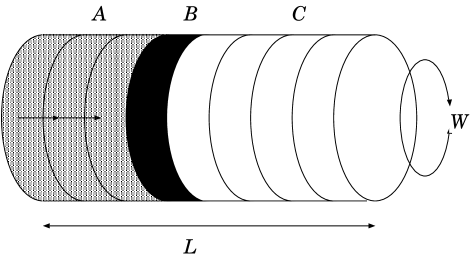
FIG. 1.: The systems we consider are of dimensions $L\times W$ where $L=2W,3W,5W,20$ and $W=2,\dots,6$. The system contains three parts: A left-hand part $A$ (shaded), an intermediate band $B$ (black) and a right-hand part $C$ (white). Actually the figure obscures that for $L=2W,3W,20$ the systems are periodical in both directions. At every DMRG step part $A$ and $B$ are contracted.

The lay-out of this paper is as follows: First we introduce the ITF. The critical behaviour of this model is discussed next. After that, we shift our attention to the DMRG. We make a link with perturbation theory and show the limitations of the method as a consequence of the environment, part $C$. Afterwards our implementation is described. Finally, we present the results of the calculations: On one hand, the accuracies achieved and on the other hand, the critical properties of the ITF.

II The ITF

Since the beginning of the 1960s, the ITF has been studied. In first instance, the purpose was to model specific materials like $KH_{2}PO_{4}$ crystals. With the introduction of the renormalization group in the 1970s, an other interest in this model has arisen. As there exist a simple relation to a classical system, the ITF is used as a vehicle to extend the knowledge of critical phenomena from classical spin systems to quantum systems. Chakrabarti, Dutta and Sen [chakrabarti] have recently summarised the properties of the ITF. For further details we refer to them. We will only mention those properties here, that are of explicit use to our calculations.

A The Model

Consider a two dimensional square lattice with length $L$ and width $W$. The lattice is periodic in both directions and each lattice site contains a spin-$\frac{1}{2}$. The Hamiltonian is given by

$${\cal H}_{ITF}=\sum_{i=1}^{L}\sum_{j=1}^{W}\left(-J{\cal S}_{i,j}^{x}({\cal S}_{i+1,j}^{x}+{\cal S}_{i,j+1}^{x})+H{\cal S}_{i,j}^{z}\right)$$ (1)

where the ${\cal S}^{\alpha}_{i,j}$ are the usual Pauli spin matrices satisfying

$$[{\cal S}_{i,j}^{\alpha},{\cal S}_{i^{\prime},j^{\prime}}^{\beta}]=2i\delta_{i,i^{\prime}}\delta_{j,j^{\prime}}\epsilon_{\alpha\beta\gamma}{\cal S}_{i,j}^{\gamma}~{}~{},~{}~{}\alpha,\beta,\gamma=x,y,z$$ (2)

As only the ratio $H/J$ is important, we fix $J$ at $J=1$ and take $H\geq 0$ ( $H\leq 0$ being equivalent).

This model is translation and reflection symmetric in both directions. Moreover, the symmetry operation ${\cal S}_{i,j}^{x}\rightarrow-{\cal S}_{i,j}^{x}$, ${\cal S}_{i,j}^{y}\rightarrow-{\cal S}_{i,j}^{y}$ and ${\cal S}_{i,j}^{z}\rightarrow{\cal S}_{i,j}^{z}$ leaves the model invariant. The operator associated with this is ${\cal S}=\exp(i\pi/2(\sum_{i,j}{\cal S}_{i,j}^{z}+LW))$. It samples the total number of spins pointing upwards and returns whether it is odd ${\cal S}=-1$, or even ${\cal S}=+1$. We call this ${\cal S}$ the spin-reversal operator. The ground state is an eigenfunction of all these symmetries operations.

If $H\rightarrow 0$, we end up with a simple 2D Ising model. The ground state is degenerate; all spins point either up or down in the ${\cal S}^{x}$-direction. The associated phase is the classical ordered phase. By taking a rotation in the lowest energy space, we can obtain states that are even in spin-reversal (${\cal S}=+1$) or odd (${\cal S}=-1$). In the other extreme, $1/H\rightarrow 0$, free spins in an external field remain. The ground state is unique and has all spins pointing down in the ${\cal S}^{z}$-direction. This is the reference state for the quantum disordered phase and has value ${\cal S}=+1$. The lowest excitation differs from the ground state by the reversal of one spin. So it belongs to the class ${\cal S}=-1$. We will extensively study the energy gap $\Delta$ between the lowest excitation (in ${\cal S}=-1$) and the ground state (in ${\cal S}=+1$); $\Delta=E_{ex}-E_{gr}$.

There is a phase transition between the classical ordered and the quantum disordered state. A clear signature of this phase transition is the disappearance of the gap $\Delta$, which occurs for a critical value $H=H_{c}$.

B Critical Behaviour

As mentioned before, the ITF is closely related to a classical Ising model. It can be mapped onto an anisotropic Ising model in one dimension higher. In the current situation the resulting classical model is of size $L\times W\times\infty$. It contains a weak coupling $K_{\perp}$ in the $L\times W$-plane and a strong Ising coupling $K_{||}$ in the remaining direction ($\exp(-K_{||})=\varepsilon H$, $K_{\perp}=\varepsilon J$ with $\varepsilon\ll 1$). Chakrabarti et al. [chakrabarti] give an overview of the procedure. For our purposes the most important consequences are:

• The correlation length $\xi$ in the strong coupling direction corresponds to the inverse of our gap $\Delta$ ($\xi\sim\Delta^{-1}$).

• The reduced temperature $t=(T-T_{c})/T_{c}$ corresponds to our reduced field $h=(H-H_{c})/H_{c}$. ($t\sim h$).

The well-known relation $\xi\sim t^{-z\nu}$ transforms into $\Delta\sim h^{z\nu}$. In the 3D anisotropic Ising model the dynamical exponent $z=1$. We use this in the further discussion. The standard finite size scaling methods as described in [cardy] can be applied here. The classical scaling relation $\xi(t,W^{-1})=b\xi(b^{1/\nu}t,bW^{-1})$, for fixed aspect ratio, $L/W=$ constant, becomes

$$\Delta(h,W^{-1})=\frac{1}{b}\Delta(b^{1/\nu}h,bW^{-1}).$$ (3)

We may set $b=W$ and obtain the scaling expression

$$W\Delta(h,W^{-1})=\Delta(W^{1/\nu}h,1),$$ (4)

showing that $W\Delta$ only depends on the combination $W^{1/\nu}h$. So for $h=0$ all lines $W\Delta$ cross at the same value;

$$W\Delta(0,W^{-1})=\Delta(0,1)$$ (5)

This gives us $H_{c}$. If we differentiate (4) with respect to $h$ and set $h=0$ afterwards, we obtain

$$\left(1-\frac{1}{\nu}\right)\log\left(\frac{W}{W+1}\right)=-\log\left(\frac{\Delta_{h}(0,W^{-1})}{\Delta_{h}(0,(W+1)^{-1})}\right).$$ (6)

From this we can extract $\nu$.

III the DMRG Method

The DMRG method was first formulated by White [white92]. As it is not a renormalization group method in the traditional sense, it could perhaps better be named an iterative basis truncation method. Gehring, Bursill and Xiang [gehring96] provide an excellent introduction in the application of the DMRG to 1D spin systems. Here we will not be so extensive. Two important features of the method are discussed and our approach is outlined.

A Limitations by the Environment

The essence of the DMRG can be described as follows: Consider a system consisting of 2 parts, $A$ and $B$. Moreover, suppose we have an approximate ground state wave function of the combined system $|\phi_{0}\rangle=\sum_{ij}\phi_{ij}|i\rangle|j\rangle$. The bases $\{|i\rangle\}$ and $\{|j\rangle\}$ do not have to be complete. We want to reduce the number of basis states in part $A$, preserving the ground state wave function $|\tilde{\phi}_{0}\rangle$ as well as possible. $|\phi_{0}\rangle$ can be expanded as

$$|\tilde{\phi}_{0}\rangle=\sum_{\alpha j}\tilde{\phi}_{\alpha j}|\alpha\rangle|j\rangle.$$ (7)

where $\{|\alpha\rangle\}$ spans only a subspace of $\{|i\rangle\}$. Preserving the ground state means that

$$\left||\phi_{0}\rangle-|\tilde{\phi}_{0}\rangle\right|^{2}\hbox{ is minimal.}$$ (8)

The solution to this problem can be obtained by means of simple algebra [white92]; Construct the density matrix $\rho_{ii^{\prime}}=\sum_{j}\phi_{ij}\phi_{i^{\prime}j}$ and select the eigenvectors $\vec{\nu}^{\alpha}$ with the largest eigenvalues $\lambda^{\alpha}$; $\vec{\vec{\rho}}\cdot\vec{\nu}^{\alpha}=\lambda^{\alpha}\vec{\nu}^{\alpha}$. The new basis is now given by: $|\alpha\rangle=\sum_{i}\nu^{\alpha}_{i}|i\rangle$.

A truncation error

$$p=1-\sum_{\alpha}\lambda^{\alpha}=\left||\phi_{0}\rangle-|\tilde{\phi}_{0}\rangle\right|^{2}$$ (9)

is introduced to give an indication of the effectiveness of the procedure. On basis of experience this truncation error is said to be a measure of the error in the calculated energy with respect to the exact result.

There is a peculiarity that was only briefly mentioned by White [white92]. Suppose we want to use this selection scheme to obtain as many states in part $A$ as we already have in part $B$, presuming that there were more states in $A$ initially. Define $|\beta_{j}\rangle=\sum_{i}\phi_{ij}|i\rangle$. The ground state can be transformed into this set;

$$|\phi_{0}\rangle=\sum_{ij}\phi_{ij}|i\rangle|j\rangle=\sum_{j}|\beta_{j}\rangle|j\rangle$$ (10)

Thus by orthonormalising the set $\{|\beta_{j}\rangle\}$ we obtain a basis set for $A$ in which the wave function can exactly be reproduced. A reformulation of this is: Consider a $|\alpha\rangle$ such that $\langle\beta_{j}|\alpha\rangle=0$ for all $|\beta_{j}\rangle$. We know that $|\alpha\rangle=\sum_{i}\nu_{i}^{\alpha}|i\rangle$, thus

$$\langle\beta_{j}|\alpha\rangle=\sum_{i^{\prime}}\phi_{i^{\prime}j}\nu^{\alpha}_{i^{\prime}}=0$$ (11)

and

$$\sum_{i^{\prime}}\rho_{ii^{\prime}}\nu_{i^{\prime}}^{\alpha}=\sum_{i^{\prime}j}\phi_{ij}\phi_{i^{\prime}j}\nu^{\alpha}_{i^{\prime}}=0.$$ (12)

$\vec{\nu}^{\alpha}$ is a zero eigenvector of $\vec{\vec{\rho}}$. Keeping the subspace spanned by the $|\beta_{j}\rangle$ would make the truncation error $p$ equal to zero. This lack of choice only becomes worse in case symmetries are implemented; not just the total number of non-zero eigenstate is fixed, but even within a specific symmetry class the number of non-zero eigenstate is dictated by the states in the environment. Later on, we will make this explicit for the systems we consider.

B The Connection with Perturbation Theory

Liang and Pang [liang94] mention that for a given accuracy, the number of states needed in a single part of the system grows exponentially with the width of the system. At the phase transition, we confirm this observation (figure 5). Moreover, both in the weak and strong field limits ($H\ll 1$ and $1/H\ll 1$), we find a fast convergence, which can be explained by perturbation theory.

Consider the quantum disordered phase. Split the Hamiltonian into a unperturbed part ${\cal H}_{0}=H\sum_{i,j}{\cal S}_{i,j}^{z}$ and a perturbation ${\cal V}=-\sum_{i,j}{\cal S}_{i,j}^{x}({\cal S}_{i+1,j}^{x}+{\cal S}_{i,j+1}^{x})$. We split the periodical, rectangular system of size $L\times W$ again in two parts; $A$ and $B$ of sizes $l\times W$ and $(L-l)\times W$ where $l$ is an arbitrary length smaller than $L$. They both contain $2W$ spins that border the other part. The unperturbed ground state $|0\rangle$ has all spins pointing down in the ${\cal S}^{z}$-direction. It is the direct product of two equivalent states restricted to $A$ and $B$; $|0\rangle=|0\rangle_{A}|0\rangle_{B}$. We know that ${\cal H}_{0}|0\rangle=-HLW|0\rangle=E_{0}|0\rangle$. Perturbation theory yields

$$|\phi_{0}\rangle=|0\rangle+\frac{1}{E_{0}-{\cal H}_{0}}{\cal V}|0\rangle+{\cal O}\left(\frac{1}{H^{2}}\right)$$ (13)

The perturbation flips a pair of neighbouring spins. This pair can be in a single part or it can cross the border between both parts. In the latter case the spins are adjacent across the boundary between part $A$ and $B$. Define $\{|a\rangle_{A}\}$ to be the set of states with the flipped pair in part $A$. Idem for $\{|b\rangle_{B}\}$. Moreover let $\{|n\rangle_{A}\}$ be the set with one spin flipped on the $n$th boundary site with $B$ and define in an equivalent manner $\{|n\rangle_{B}\}$. The perturbation expansion can now be rewritten

$$|\phi_{0}\rangle = |0\rangle_{A}|0\rangle_{B}+\frac{1}{2H}\left(\sum_{a}|a\rangle_{A}|0\rangle_{B}+\sum_{b}|0\rangle_{A}|b\rangle_{B}+\sum_{n}|n\rangle_{A}|n\rangle_{B}\right)+{\cal O}\left(\frac{1}{H^{2}}\right)$$ (14)

$$= \left(|0\rangle_{A}+\frac{1}{2H}\sum_{a}|a\rangle_{A}\right)\left(|0\rangle_{B}+\frac{1}{2H}\sum_{b}|b\rangle_{B}\right)+\frac{1}{2H}\sum_{n}|n\rangle_{A}|n\rangle_{B}+{\cal O}\left(\frac{1}{H^{2}}\right)$$ (15)

As $H\gg 1$, it is necessary to reproduce all these terms for an accuracy which is equivalent to the first order perturbation theory. The minimal number of states needed in part $A$ is therefore $1$ for the first term in (15) plus $2W$ for all the boundary terms. We have confirmed this prediction explicitly in both the small and large $H$ limit ( $H=1/50,50$).

The same line of reasoning also holds for the second and higher order perturbation terms. We expect for an error comparable to the $n$th order perturbation theory that $m\sim W^{n}$, $\delta E\sim(1/H)^{n}$. This is always an upper bound for number of states $m$ needed, $m<W^{n}$ for a given accuracy $\delta E\sim(1/H)^{n}$. Only when the different orders in perturbation theory become distinguishable in size - the limit of large $H$- the equivalence holds.

C Exploiting the Symmetries

We consider systems of sizes $L\times W$. The length $L$ is either a multiple of $W$, $L=2W,3W,5W$, or it is fixed, $L=20$. The width $W$ is varied from $W=2$ to $W=6$. The maximal system we study thus contains $6*30=180$ spins. For $L=2W,3W$ and $20$ a torus is constructed by imposing periodical boundary conditions in both directions. For $L=5W$ the system follows the figure 1 more genuinely; it is periodical in the width-direction and open in the length-direction. The system is split in a left-hand and a right-hand part, both containing $m$ states. A intermediate band, containing the complete basis of $2^{W}$ states, separates them. This is depicted in figure 1.

The Hamiltonian of such a system contains many symmetries that we can incorporate in our calculation. The general form of the included symmetry operators is that they are the direct product of three components. Each component acts on one part of the system only. For example, consider the translation operator ${\cal T}$ in the width-direction. This operator is the direct product of three translations in the individual parts; ${\cal T}={\cal T}_{A}{\cal T}_{B}{\cal T}_{C}$. The same holds for the reflection ${\cal R}$ in the same direction,${\cal R}={\cal R}_{A}{\cal R}_{B}{\cal R}_{C}$, and the spin-reversal operator ${\cal S}=\exp(i\pi/2(\sum_{i,j}{\cal S}^{z}_{i,j}+LW))={\cal S}_{A}{\cal S}_{B}{\cal S}_{C}$.

The ground state $|\phi_{0}\rangle$ of the system is translational, reflection and spin-reversal invariant; ${\cal T}|\phi_{0}\rangle={\cal R}|\phi_{0}\rangle={\cal S}|\phi_{0}\rangle=|\phi_{0}\rangle$. For systems of infinite size in the classical ordered region ($L,W\rightarrow\infty$ and $H\ll 1$), it will become degenerate with a state that is spin-reversal anti-symmetric. In order to take advantage of the symmetries, the bases of part $A$, $B$ and $C$ are chosen to be eigenvectors of the symmetry operators ${\cal T}$ and ${\cal S}$. ${\cal R}$ is used later on. So if $\{|a\rangle\}$, $\{|b\rangle\}$, $\{|c\rangle\}$ are the bases of the individual parts ( not to be mixed-up with the notation used in (15)) then

$${\cal T}_{A}|a\rangle=e^{ik_{a}}|a\rangle~{}~{},~{}~{}{\cal S}_{A}|a\rangle=s_{a}|a\rangle.$$ (16)

Similar relations hold for the other two sets. Thus

$$|\phi_{0}\rangle=\sum_{abc}\phi_{abc}|a\rangle|b\rangle|c\rangle$$ (17)

and application of the symmetry operations together with (16) yields:

$$k_{a}+k_{b}+k_{c} = 0~{}\hbox{mod}~{}2\pi,$$ (18)

$$s_{a}s_{b}s_{c} = 1.$$ (19)

It is also possible to set up the program to find the lowest state in other symmetry classes by forcing other values than $0$ and $1$ in the equations above.

The Hamiltonian can be written as the sum of Hamiltonians within the separate parts: ${\cal H}_{A},{\cal H}_{B}$ and ${\cal H}_{C}$ combined with interactions between parts: ${\cal H}_{AB},{\cal H}_{BC}$ and ${\cal H}_{CA}$; ${\cal H}={\cal H}_{A}+{\cal H}_{B}+{\cal H}_{C}+{\cal H}_{AB}+{\cal H}_{BC}+{\cal H}_{CA}$. To show how to implement the symmetries, we will discuss one element of both types.

First ${\cal H}_{A}$: It is translational and spin-reversal invariant, thus

$$\langle a^{\prime}|{\cal H}_{A}|a\rangle = \langle a^{\prime}|{\cal T}_{A}^{-1}{\cal H}_{A}{\cal T}_{A}|a\rangle=e^{i(k_{a}-k_{a^{\prime}})}\langle a^{\prime}|{\cal H}_{A}|a\rangle$$ (20)

$$= \langle a^{\prime}|{\cal S}_{A}^{-1}{\cal H}_{A}{\cal S}_{A}|a\rangle=s_{a^{\prime}}s_{a}\langle a^{\prime}|{\cal H}_{A}|a\rangle$$ (21)

$$= \langle a^{\prime}|{\cal H}_{A}|a\rangle\delta_{s_{a^{\prime}},s_{a}}\delta_{k_{a^{\prime}},k_{a}}.$$ (22)

It only contains elements within symmetry classes, as one would expect.

Second ${\cal H}_{AB}$: Once again, it is translational and spin-reversal invariant. Moreover it can be written as

$${\cal H}_{AB} = -\sum_{n=1}^{W}{\cal S}^{x}_{l,n}{\cal S}^{x}_{l+1,n}$$ (23)

$$= -\sum_{n=1}^{W}({\cal T}_{A}{\cal T}_{B})^{-n+1}{\cal S}^{x}_{l,1}{\cal S}^{x}_{l+1,1}({\cal T}_{A}{\cal T}_{B})^{n-1}$$ (24)

where $l$ is the length of part $A$. ${\cal S}_{i,j}^{x}$ flips a spin, so ${\cal S}_{i,j}^{x}{\cal S}+{\cal S}{\cal S}_{i,j}^{x}=0$. Inserting this and (16) in (24) gives

$$\langle a^{\prime}|\langle b^{\prime}|{\cal H}_{AB}|a\rangle|b\rangle = -W\langle a^{\prime}|{\cal S}_{l,1}^{x}|a\rangle\langle b^{\prime}|{\cal S}_{l+1,1}^{x}|b\rangle\cdot$$ (27)

$$\delta_{k_{a^{\prime}}+k_{b^{\prime}},k_{a}+k_{b}}\cdot$$

$$\delta_{s_{a^{\prime}},-s_{a}}\delta_{s_{b^{\prime}},-s_{b}}.$$

This substantially reduces the computational effort. Finally: the reflection operator ${\cal R}$ is used to make matrix elements like $\langle a^{\prime}|{\cal S}_{l,1}^{x}|a\rangle$ real. Naturally we could have used this last symmetry ${\cal R}$ more, but it only reduces the effort by a factor of 4 while making the program far more complex.

D The Implementation

Now we focus on the procedure itself. It is tempting to use the 1D DMRG method directly: a site is replaced by a band. The ground state $|\phi_{0}\rangle$ of the entire system ABC is calculated and the optimal basis for block AB is selected through the density matrix. However, one runs in severe difficulties as a consequence of the first remark on the DMRG. It is instructive to reveal the reason: Using the notation above, we define $|\beta_{c}\rangle=\sum_{ab}\phi_{abc}|a\rangle|b\rangle$. We know that ${\cal T}|\phi_{0}\rangle={\cal S}|\phi_{0}\rangle=|\phi_{0}\rangle$, thus

$${\cal T}_{A}{\cal T}_{B}|\beta_{c}\rangle = e^{-ik_{c}}|\beta_{c}\rangle$$ (28)

$${\cal S}_{A}{\cal S}_{B}|\beta_{c}\rangle = s_{c}|\beta_{c}\rangle$$ (29)

The distribution over the symmetry classes in part $C$ forces the selected states in block $AB$ to be in “conjugate”-classes. To overcome this problem, we need to increase the number of states in part $C$. In that case we can really make a selection and shift into important symmetry classes.

In the 1D procedure the solution is to add one extra site to the environment. The number of states in the environment is then doubled. In our set-up this would correspond to adding an extra band between B and C. This is computational far too expensive. We now introduce variants on White’s infinite-size and finite-size algorithms [white92] that increase the number of states in the part C.

First we consider our infinite size approach. We only have to describe one step in the process as it is an inductive method. We have a basis of $m$ states for a system of length $l$.

• We construct the combined system as depicted in figure 2-a by taking this basis in part $A$ and $C$ together with the complete basis in the intermediate band $B$. ($L=2l+1$)

• We calculate the ground state $|\phi_{0}\rangle$ and obtain $m$ basis states for a system of length $l+1$ by orthonormalising $\{|\beta_{c}\rangle\}$.

• Suppose that block $AB$ has $f$ symmetry classes. To every symmetry class we add $m/f$ basis states constructed randomly from the $m2^{W}$ states in $A$ and $B$. We end up with $m+f\cdot m/f=2m$ basis states for a system of length $l+1$.

• In part $A$ we now take the $m$ basis states for a system of length $l$ and in part $C$ we take the newly constructed $2m$ states for length $l+1$. ($L=2l+2$) This yields the configuration in figure 2-b.

• We calculate the ground state $|\phi_{0}\rangle$ and obtain $2m$ basis states for length $l+1$ by orthonormalising $\{|\beta_{c}\rangle\}$. We replace the basis of part $C$ by this basis and repeat this step a couple of times ($\sim 3$).

• We select from the $2m$ basis states for length $l+1$ $m$ states on basis of the density matrix.

Now we have returned to the original situation with the exception that $l$ has increased by one. The new ingredient is thus to add $m$ random states to the basis and iterate until the result has converged.

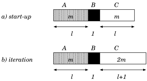
FIG. 2.: A inductive step in the infinite-size procedure consists of a start-up to obtain an initial approximation for states in a system of length $l+1$ and iterative calculations to make the basis converge. The numbers in the rectangle are the number of states in the parts. The intermediate band B always contains the complete basis of $2^{W}$ states.

In the same line our finite size approach lies. Suppose we have basis sets of $m$ states for lengths $l$,$L-l-1$ and $L-l-2$, where $L$ is now fixed and independent of $l$.

• We take the basis for $l$ in part $A$, the basis for $L-l-1$ in part $C$ and the complete basis of the band in part $B$. See figure 3-a.

• We calculate the ground state $|\phi_{0}\rangle$ and obtain a basis for length $l+1$ by orthonormalising $\{|\beta_{c}\rangle\}$.

• In the same way as in the infinite-size algorithm we add $m$ randomly chosen states to this basis.

• In part $C$ we take the $2m$ basis states for length $l+1$ and in part $A$ the $m$ states for length $L-l-2$. This is depicted in the first of the two pictures in figure 3-b.

• We calculate the ground state $|\phi_{0}\rangle$ and obtain $2m$ basis states for $L-l-1$.

• In part $C$ we take the $2m$ basis states for length $L-l-1$ and in part $A$ the $m$ states for length $l$; see the second picture in figure 3-b.

• We calculate the ground state $|\phi_{0}\rangle$ and obtain $2m$ basis states for $l+1$. These last four steps are repeated a couple of times ($\sim 3$)

• We select from the $2m$ basis states for length $l+1$ $m$ states on basis of the density matrix.

Once again we have returned to our starting position while increasing the length $l$ by one. By sweeping through the system we can therefore systematically improve the basis. This method convergences at a similar speed as the 1D approach; After 3 sweeps through the system the final result is achieved.

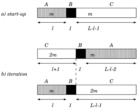
FIG. 3.: A inductive step in the finite-size procedure also consists of a start-up to obtain an initial approximation for states in a system of length $l+1$. Afterwards we move back and forth between lengths $l$ and $l+1$ to make this converge.

The computational effort scales as $m^{3}L\frac{2^{W}}{W}$. In general $m\gtrsim 2^{W}$. This clarifies the bound on the width. The alternative is to follow Liang, Pang [liang94] and White [white96] by adding one site per step. We can then still use ${\cal S}$. The calculation would scale as $m^{3}L\frac{W^{2}}{2^{2}}$. Our approach includes the symmetry requirements of the ground state and up to $W\sim 8$ it is similar in speed as theirs. Applying our method to models where the number of particles or total spin is conserved instead of ${\cal S}$, the calculations can been substantially reduced and systems of widths $W>6$ are pulled within reach.

The largest calculation, $W=6$, $L=18$, $m=200$ took 48h of computer time per $H$-value (at 462 SPECfp92). To determine the gap $\Delta$ two such points are needed (${\cal S}=+1$ and ${\cal S}=-1$).

IV Results

We have performed two kinds of calculations: First, we made a check on the accuracy of the method. Second, we have calculated the gap $\Delta$ for various widths $W$, aspect ratio’s $L=xW$ and fields $H$ in order to find through finite size scaling the phase transition point $H_{c}$ and the critical exponent $\nu$.

A The Accuracy of the Energies.

The strict method to determine the error in the energy $\delta E_{m}$ for given number of states $m$ is to compare the results $E_{m}$ with the exact value $E_{gr}$; $\delta E_{m}=E_{m}-E_{gr}$. This would limit us to small systems of sizes comparable to $6\times 6$. In the literature [liang94] it is noted that the error $\delta E$ decreases exponentially with the number of states $m$ included. We confirm that statement explicitly for these small systems. Moreover we use this feature to test the accuracy for far larger systems. The energy $E_{m}$ is compared with the result for a larger number of states. For instance $m<128$; $\delta E_{m}\approx E_{m}-E_{128}$. The error $\delta E_{m}$ is largest near the phase transition as can be seen in figure 4.

FIG. 4.: The accuracy of the DMRG method for different of states $m$ (numbers in graph) as function of the field $H$. The system is periodical in both directions with dimensions $W=4$ and $L=20$. The reference value is taken from a DMRG calculation with $m=64$.

As the phase transition occurs near $H=3$, we take $H=3$ as an example to study the dependence of the error $\delta E$ on the width $W$. The error $\delta E_{m}$ increases exponentially with growing width $W$ (figure 5).

FIG. 5.: The accuracy of the DMRG method for given number of states $m$ (numbers in graph) as function of the width $W$. $H=3$ and $L=20$. The system is periodical in both directions. The reference value is taken from a DMRG calculation with $m=128$.

B The Phase Transition and the Critical Exponent.

The phase transition point $H_{c}$ is determined through equation (5). We plot $W\Delta$ versus $H$ (figure 6 and 7). The curves would intersect precisely at $H_{c}$, if it were not for corrections to scaling. These become quite large when $W=2,3$. Afterwards we use formula (6) to obtain $\nu$ at the intersection of the curves for consecutive widths $W$. The results are listed in table I. For $W=6$ and $L=2W,3W$ we are at the limit of our precision, when we take $m=128$ states. We therefore set $m=200$ in this case.

Apart from these periodical systems, we have also considered systems where the periodical connection between $A$ and $C$ is removed. The removal of this boundary connection has two effects: First, the accuracy of the calculated energies will increase substantially as the size of the interacting boundary is halved. Second, the corrections to scaling will increase. To make up for this second effect, we have to resort to fairly large systems; $L=5W$. This is depicted in figure 8.

From the values in table I we note that the corrections to scaling for $\nu$ are still fairly large for these system sizes ($\sim 5\%$). We found that these corrections could not be compensated by introducing an irrelevant scaling field in the relation (3).

FIG. 6.: The scaled gap $W\Delta$ as function of the field $H$ for aspect ratio $L=2W$. $W=2,3,4,5,6$. The curves become steeper with increasing width $W$. The crossings for consecutive widths are encircled. The system is periodical in both directions. $m=128$, for $W=2,3,4,5$ and $m=200$ for $W=6$)

FIG. 7.: Idem as figure 6 with now the ratio $L=3W$.

FIG. 8.: The scaled gap $\Delta W$ for systems with open boundary conditions in the length-drections and periodical in the width-direction. $L=5W$ and $m=64$.

	$L=2W$		$L=3W$		$L=5W$
$W$	$H_{c}$	$\nu$	$H_{c}$	$\nu$	$H_{c}$	$\nu$
2-3	3.113	0.74	3.110	0.73	3.101	0.74
3-4	3.068	0.69	3.067	0.68	3.062	0.69
4-5	3.054	0.67	3.053	0.67	3.051	0.67
5-6	3.049	0.66	3.047	0.65	3.046	0.66

TABLE I.: The phase transition point $H_{c}$ and the critical exponent $\nu$. We take $H_{c}$ to be the value where $W\Delta(W^{-1})=(W+1)\Delta((W+1)^{-1})$. $\nu$ is calculated through equation (6). The first two aspect ratio’s $L=2W,3W$ are with periodical boundary conditions, the last $L=5W$ is with open boundary conditions in the length-direction.

V Conclusion

In this paper we have presented an adaption of the DMRG method to two dimensional spins systems. We follow the route of adding complete bands instead of single sites to the system. The latter was done by Liang, Pang [liang94] and White [white96]. This modification allows us to force a translational symmetry in the width-direction. The advantage of implementing this symmetry is that a ground state with specific translational properties can be targeted. Moreover, the space in which the ground state is sought is reduced substantially. This is especially useful in systems with Goldstone modes or similar gapless excitation spectra where the lowest excitations belong to different symmetry classes than the ground state.

The computational effort still remains similar to the approach of adding single sites as the larger space of the band ($2^{W}$ instead of $2$) is offset by three reductions: First, the ground state can be written more compactly (a factor $W$ reduction). Second, we only need to apply one operator ${\cal S}^{x}$ per boundary instead of $W$ operators. Third, the sub-system (part A) grows with a full band instead of a single site per step (factor $W$).

We have only considered systems of widths upto $W=6$. In models where the total spin or the number of particles is conserved, we can go to larger widths.

We observe that at criticality, the number of states $m$ needed for a given accuracy $\delta E/E$ grows exponentially with the width $W$, in full agreement with Liang and Pang [liang94]. Moreover, we have proven that far enough from the phase transition the method will reproduce perturbation theory.

The procedure does not get stuck at local minima as was sometimes experienced by White and Scalapino [white97].

The gap $\Delta$ we have calculated is a nice example of the use of symmetry classes. The results for the critical properties, $H_{c}=3.046$ and $\nu=0.66$, are in reasonable agreement with the series expansions of Pfeuty and Elliott [pfeuty77] and with the cluster Monte Carlo calculations of Blöte [bloete97].

As yet, this method is not as accurate as the more traditional methods like Monte Carlo simulations. The accuracy could be improved when a larger width could be handled by including several hunderds of states. At present this would require the use of a super-computer. Still it has to be stressed that the DMRG can handle problems that are out of reach of Monte Carlo simulations due to the “sign-problem”.

Acknowledgement. We thank H. W. J. Blöte for guiding us through the classical analogue and supplying the state-of-the-art value of the critical field $H_{c}$. We are indebted to W. van Saarloos for his continued interest in the problem and his suggestions for the scaling analysis.