Driven Dynamics of Periodic Elastic Media in Disorder

Abstract

We analyze the large-scale dynamics of vortex lattices and charge density waves driven in a disordered potential. Using a perturbative coarse-graining procedure we present an explicit derivation of non-equilibrium terms in the renormalized equation of motion, in particular Kardar-Parisi-Zhang non-linearities and dynamic strain terms. We demonstrate the absence of glassy features like diverging linear friction coefficients and transverse critical currents in the drifting state. We discuss the structure of the dynamical phase diagram containing different elastic phases very small and very large drive and plastic phases at intermediate velocity.

I Introduction

Periodic structures driven through a random environment have become a paradigm for the statistical mechanics of non-equilibrium processes. The beginning of the study of this phenomenon in the context of charge density wave (CDW) dynamics was marked by the development of several pioneering and elegant concepts (see [1] for a review), in particular the description of the depinning transition in terms of critical phenomena [2]. Yet it was hard to foresee the subsequent growth of what seemed to be a simple although a subtle subject into a fascinating multidisciplinary branch of statistical physics. The resurgence of interest was related to the discovery of high temperature superconductors (HTS) where the motivation was driven also by the technological quest for the description of transport properties of HTS.

The understanding of the remarkable effects displayed by driven vortex lattice involved a diversity of concepts drawn from various branches of contemporary physics ranging from polymer physics and spin glasses to nonlinear stochastic equations and turbulence, as well as the invention of new concepts of non-equilibrium physics of disordered media (see [3]). In recent years much theoretical effort has been expended to advance our knowledge of the driven dynamics of disordered media. Yet in spite of impressive achievements there remains a vast amount of fundamental open questions with the depth and subtleties still to be revealed. In this work we develop a regular approach to the description of periodic media driven through a quenched random environment that will hopefully enable to put subsequent research endeavors on a firm standard basis.

Statics of disordered elastic periodic systems

The subtle dynamic properties of dirty media are governed by the interplay among thermal fluctuations, driving force, and quenched disorder. To gain better insight into the dynamics we first discuss briefly the statics of weakly disordered elastic periodic systems. These include CDW, vortex lattices (VL), vortex arrays in Josephson junctions, domain walls, dislocations in solids, Wigner crystals, and many others. The common feature of the above systems is that, although the weakness of pinning suggests the purely elastic Hamiltonian as a starting point, the disorder-distorted system possesses a huge number of meta-stable states and the ground state is infinitely degenerate. This dooms to eventual failure direct attacks on the asymptotic large-scale behavior based on a straightforward perturbation theory with respect to disorder.

The first and decisive step for an approach by statistical physics to such systems was made in the remarkable work of Larkin [4]. The pioneering ideas of this work were later cast into the collective pinning theory [5, 6, 7] and basically determined the further development of the field. It was recognized in [4] that pinning can be treated perturbatively in the domain of the distorted lattice belonging to a single meta-stable state generated by disorder. Such a coherently pinned domain is called the correlated volume and the pinning energy stored in such a domain determines the crucial characteristic of the pinned system: the critical depinning force.

The key quantity characterizing the system is the degree of distortion of the elastic system by disorder, the roughness $w({\bf r})=\overline{\langle[{\bf u}({\bf r})-{\bf u}({\bf 0})]^{2}\rangle}$, where ${\bf u}({\bf r})$ is the displacement of a vortex from its undistorted position ${\bf r}$. Within the domain $w(r)\leq\xi^{2}$, where $\xi$ is the characteristic spatial scale of variations of the random potential, the pinning force ${\bf f}$ has only a negligible dependence on the displacements ${\bf u}$. This implies that this domain is pinned coherently and lies in the single valley of the effective potential landscape of the system. The roughness within the correlation volume grows as $w(r)\propto r^{2\zeta}$ with the so-called wandering or roughness exponent $\zeta$ that takes the value $\zeta=\frac{4-d}{2}$ in the Larkin regime ($d$ is the dimensionality of the lattice). Since different Larkin domains are pinned independently one could conclude that pinning, however weak, destroys the long-range order of the lattice for $d<4$.

As soon as the relative displacement of vortices exceeds the disorder correlation length, the spatial variation of the pinning forces becomes important. The vortices start to feel that they are in a random potential having many meta-stable states rather than in a random force field. Therefore the perturbative result would overestimate the actual roughness of the lattice. On intermediate scales where $\xi^{2}\leq w(r)\leq a^{2}$ and $a$ is the lattice constant the system adjusts itself to the multi-valley potential relief. This regime is referred to as the random manifold regime [8] and the roughness exponent becomes smaller than in the Larkin regime. On these scales the periodicity of the medium is not yet of significance. The region of the largest scales, where lattice displacements exceed the lattice constant, $a^{2}\leq w(r)$, and the periodic nature comes into play, was first investigated by Nattermann [9] who found, by the renormalization group approach, that at large distances pinning of the VL is equivalent to pinning of CDW and that displacements grow only logarithmically, $w(r)\propto\ln(r)$. The above results were confirmed later by variational replica approaches [10, 11, 12, 13].

Structures with logarithmic roughness are well known in the physics of surfaces and 2D crystals. The logarithmic roughness implies that the system retains its periodic character and Bragg peaks in the structure factor $S({\bf q})$, the singularities however have an algebraic character, $S({\bf q})\propto|{\bf q}-{\bf Q}|^{-\nu}$, (${\bf Q}$ is a reciprocal lattice vector) rather than the $\delta$-function-like character as in ordinary crystals or Lorentzian character in liquids [14, 15, 16]. This algebraic behavior is a characteristic feature of quasi-long-range crystalline order.

The roughness of the lattice structure implies a ruggedness of the potential landscape of the system and the existence of infinitely high barriers separating the different meta-stable states, which is the characteristic feature of glassy systems (see [3]). This was realized in a seminal work by M.P.A. Fisher [17] who identified the VL distorted by disorder as a glassy structure and called it the vortex glass. It is important to stress that the derivation of the above features was based on the elastic nature of disordered lattices.

The stability of the elastic vortex glass with respect to the formation of topological defects (dislocations) was questioned by Fisher, Fisher and Huse [18] who stated that dislocations are to be generated at the scales where the roughness becomes of order the vortex spacing and that therefore the elastic description of the vortex glass fails. In spite of the fact that the correctness of the arguments of [18] was questioned in its turn (the energy of the dislocation formation was underestimated and the logarithmic smoothness of the lattice on large scales was overlooked), the image of the vortex glass as a dislocation saturated medium became widespread. Arguments demonstrating the self-consistency of the elastic vortex glass approach (as long as the disorder is weak enough) were presented in [13, 19, 20]. Thus the existence of a weak disorder-induced elastic vortex glass free of topological defects can be considered as well established. Recalling that a logarithmically rough medium shows algebraic Bragg peaks, Giamarchi and Le Doussal [13] proposed to call the vortex lattice deformed by disorder a “Bragg glass.” This name gained popularity among the specialists and replaced the somewhat compromised “vortex glass” in their technical jargon. The latter terms is now reserved for the topologically disordered vortex solid phase.

Dynamics of disordered elastic periodic systems

The main feature of the driven dynamics in a random environment is the existence of the pinning threshold: at zero temperature the system remains pinned if the drive does not exceed a certain threshold value $f_{c}$, the critical pinning force, and slides if $f>f_{c}$. At finite temperatures the sharp transition is rounded by thermal fluctuations and is not very well defined. Nevertheless, one can keep the notion of a temperature dependent critical force $f_{c}(T)$ as the force separating the pinning dominated regime with slow thermally activated dynamics or creep at low force $f\ll f_{c}$ from the fast sliding one at $f\gg f_{c}$.

Motion of the system in the creep regime occurs via thermally activated jumps over energy barriers separating different meta-stable states. The size of the typical energy barrier as a function of the driving force can be related by scaling arguments to structural features of the system, in particular its roughness. This was done in [21] for driven elastic manifolds and it was found that the barriers controlling the motion diverge algebraically at small driving forces as $U(f)\propto 1/f^{\mu}$, where $\mu=(2\zeta-1)/(2-\zeta)$. The approach of [21] was extended from continuous media to the creep of vortex lattices in [8, 9]. The divergence of the activation barriers implies a non-linear response of the system to small forces and leads to the identification of the low-temperature vortex state as a glassy phase, since such a non-linear response is a hallmark of the glassy system.

The understanding of the critical behavior at the depinning threshold has seen remarkable progress[22, 23, 24] since the first work by D.S. Fisher [2].

The high-velocity sliding of the periodic systems was long considered as the most “easy-to-understand” regime. The outburst of the interest in the flow regime at large driving forces well above the depinning threshold was triggered by the prediction [25] of dynamic phase transitions between plastic sliding in the nearest vicinity of depinning and coherent motion of the crystalline structure at high drives. Already early experiments [26] have shown that a moving vortex lattice has a higher degree of crystalline order than a pinned vortex lattice. These studies have been refined recently [27, 28] to identify the different dynamical regimes.

The non-equilibrium phase transition predicted in Ref. [25] is expected to occur in systems with sufficiently strong disorder, where depinning is accompanied by the massive production of topological defects [29]. The structural order improves at large driving forces because the system experiences disorder forces that are temporally fluctuating in the moving frame. In this sense the effect of disorder resembles the thermal noise of a heat bath. However, this comparison does not carry too far, since the quenched nature of the disorder still implies infinite-ranged spatio-temporal correlations of the effective force in the moving frame.

Balents and Fisher [30] used scaling arguments to extend the concept of the non-equilibrium “freezing” transition of Ref. [25] to CDW and have shown that true long-range order is restored at large velocities only in $d>3$. Thus the critical dimension is reduced by one in comparison to the static case. For $d\leq 3$ the CDW phase, which is the analog of the vortex displacement, is still rough even even at the largest velocities, whereas a temporal order resulting in narrow-band noise may still persist.

Giamarchi and Le Doussal [31] addressed the question of spatial large-scale order in the driven VL. They argued that the transverse periodicity of the system leads to glassy features of the driven phase. It was argued, in particular, that on the largest scales the driven lattice retains a logarithmic roughness in the directions transverse to the velocity for $2<d\leq 3$. In the direction parallel to the velocity the roughness is expected to be even algebraic as for driven CDW [32, 33] in contrast to the static case, where roughness is logarithmic. One of the manifestations of the transverse glassiness suggested according to Ref. [31] would be the existence of diverging transverse barriers. This brings to mind the early observation of Schmid and Hauger [34] who have performed a lowest-order perturbative calculation for the pinning force and noticed a discontinuity in the transverse I-V characteristic in a sliding state.

Notice that in comparison to the equilibrium situation in the absence of driving forces, the approach to the physics at large velocities is even more intricate because of the non-equilibrium nature of the driven state. Although important predictions about this state have already been formulated, a systematic approach is still lacking.

In this paper we develop such a systematic approach to the driven dynamics of dirty periodic media on the basis of the Martin-Siggia-Rose (MSR) formalism. The MSR formalism provides a powerful tool to access the largest scales and to treat the immediate vicinity of the depinning transition. Although the complete description should include the derivation of renormalization group equations, we will show that a number of important conclusions concerning the properties of the driven state can be successfully achieved even within the framework of the dynamic perturbative approach. For large velocities $v$ the small parameter for the expansion is $\Delta_{0}/(\eta^{2}v^{2}\xi^{d+2})$ where $\Delta_{0}$ is the $d$-dimensional spatial integral of the potential correlator of a width $\xi$, and $\eta$ is the friction coefficient.

Summary of results

Using a coarse-graining procedure for the dynamics of periodic media, we find that their large-scale behavior is governed by an effective equation of motion

$$\eta_{\alpha\beta}^{*}\dot{u}_{\beta} = D_{\alpha\beta}^{*}u_{\beta}+F_{\alpha}-F_{\alpha}^{{\rm fr}*}+\frac{1}{2}\lambda_{\alpha\beta\gamma ab}^{*}[\partial_{a}u_{\beta}][\partial_{b}u_{\gamma}]$$ (2)

$$+\xi_{\alpha}^{*}+f_{\alpha}^{*}({\bf r}+{\bf v}t+{\bf u})~{}.$$

Renormalized parameters carry an asterisk to distinguish them later on from the unrenormalized (bare) ones. Under this procedure the parameters become anisotropic since the velocity identifies a particular spatial direction.

All components of the friction coefficient $\eta^{*}$ are found to be finite. Therefore glassy features, which in general appear as a divergence of such coefficients, are absent. The elastic dispersion that reads $D^{*}_{\alpha\beta}({\bf q})=-i\chi^{*}_{\alpha\beta a}q_{a}+\kappa^{*}_{\alpha\beta ab}q_{a}q_{b}$ in Fourier space, includes besides elastic constants $\kappa$ also stress terms $\chi$ after coarsening.

Due to pinning and dissipative effects on spatial scales smaller than the coarse-grained cutoff scale (with momenta larger than $\Lambda^{<}$), the velocity-dependence of the friction force $F^{{\rm fr}*}$ becomes non-linear.

The fourth term in Eq. (2) is a Kardar-Parisi-Zhang (KPZ) non-linearity [35] $\lambda^{*}$, which is absent in the bare dynamics, is generated by disorder. It is an anisotopic generalization of the term $\frac{1}{2}\lambda({\mathchoice{{\hbox{\boldmath$\displaystyle\nabla$}}}{{\hbox{\boldmath$\textstyle\nabla$}}}{{\hbox{\boldmath$\scriptstyle\nabla$}}}{{\hbox{\boldmath$\scriptscriptstyle\nabla$}}}}u)^{2}$ familiar from surface growth and Burger’s equation.

The pinning force $f^{*}$, which was simply the gradient of a random potential in the bare case, acquires a more virulent random-force character with a correlator

$$\phi^{*}_{\alpha\beta} = \int_{\bf R}\overline{f_{\alpha}^{*}({\bf R})f^{*}_{\beta}({\bf 0})}~{},$$ (4)

$$\phi^{*}_{xx} \approx \frac{\Delta_{0}^{2}}{\xi^{4+d}\eta^{2}v^{2}}~{},$$ (5)

$$\phi^{*}_{yy} \approx \frac{a^{2}\Delta_{0}^{2}}{\xi^{3+d}c\eta v}~{}{\rm for}~{}d>3~{},$$ (6)

$$\phi^{*}_{yy} \approx \frac{a^{2}\Delta_{0}^{2}}{\xi^{3+d}c\eta v}(a\Lambda^{<})^{d-3}~{}{\rm for}~{}d<3$$ (7)

for large velocities $v\gg c\xi/(\eta a^{2})$ with a typical elastic constant $c$. One sees that the variance of the components perpendicular to the velocity diverges in $d\leq 3$ as the coarse-graining cutoff $\Lambda^{*}\to 0$.

The effective thermal noise $\xi^{*}$ describes in general an effective heat bath with a temperature that is increased due to shaking effects exerted by the pinning on the medium.

$$\vartheta_{\alpha\beta}^{*} = \int_{t\bf r}\langle\xi^{*}_{\alpha}({\bf r},t)\xi^{*}_{\beta}({\bf 0},0)\rangle~{},$$ (9)

$$\vartheta^{*}_{xx} \approx \vartheta+\frac{\Delta_{0}}{\xi^{2+d}\eta^{2}v^{2}}\vartheta~{},$$ (10)

$$\vartheta^{*}_{yy} \approx \vartheta+\frac{a^{2}\Delta_{0}}{\xi^{3+d}c\eta v}\vartheta~{}{\rm for}~{}d>3~{},$$ (11)

$$\vartheta^{*}_{yy} \approx \vartheta+\frac{a^{2}\Delta_{0}}{\xi^{3+d}c\eta v}(a\Lambda^{<})^{d-3}\vartheta~{}{\rm for}~{}d<3~{}.$$ (12)

In the non-equilibrium case this effective “temperature” is defined as the integral over the correlator of $\xi^{*}$, that can be distinguished from pinning forces by the temporal decay of its correlations. The behavior of $\vartheta^{*}$ and $\phi^{*}$ is very similar, they show the same type of divergence for $\Lambda^{<}\to 0$. Since this divergence comes from small momenta, it is a measure for the strong fluctuations of the medium on large scales only.

The disorder generated stress couplings $\chi$, the KPZ non-linearities and the random forces are specific non-equilibrium terms that are absent in the equation of motion before coarse-graining.

From the effective equation of motion (2) the displacement fluctuations are found to roughen the medium in dimensions $d\leq 3$ with high anisotropy for directions parallel and perpendicular to the velocity (which we choose to be parallel to the $x$-axis). The anisotropy manifests itself in two distinct features of the displacement correlations: (i) The components of the displacement field perpendicular to ${\bf v}$ exhibit stronger fluctuations than the components parallel to ${\bf v}$. (ii) The relative displacement increases faster in perpendicular directions than in the parallel direction.

The former feature, obtained below within perturbation theory for the elastic medium, can be understood qualitatively already from a single-particle picture in analogy to the consideration that led to the notion of the shaking temperature, describing the disorder-induced increase of the effective system temperature [25]. To this end we consider a particle moving in a disorder potential $V$ with Gaussian correlations $\overline{V({\bf R})V({\bf 0})}\sim{\Delta_{0}}\xi^{-d}e^{-R^{2}/(2\xi^{2})}$. A particle starting at ${\bf R}(t=0)=0$ moves with an average velocity ${\bf v}\approx{\bf F}=F{\hat{\bf x}}$ following an over-damped equation of motion $\eta\dot{\bf R}={\bf F}-{\mathchoice{{\hbox{\boldmath$\displaystyle\nabla$}}}{{\hbox{\boldmath$\textstyle\nabla$}}}{{\hbox{\boldmath$\scriptstyle\nabla$}}}{{\hbox{\boldmath$\scriptscriptstyle\nabla$}}}}V({\bf R})\approx\eta{\bf v}-{\mathchoice{{\hbox{\boldmath$\displaystyle\nabla$}}}{{\hbox{\boldmath$\textstyle\nabla$}}}{{\hbox{\boldmath$\scriptstyle\nabla$}}}{{\hbox{\boldmath$\scriptscriptstyle\nabla$}}}}V({\bf v}t)$. The components of its displacement ${\bf u}(t)={\bf R}(t)-{\bf v}t$ parallel and perpendicular to ${\bf v}$ have a variance that grows differently as a function of time. When the effect of the pinning forces is integrated over time (i.e. along the direction of motion of the particle), the force component parallel to the direction of motion is “recognized” as the gradient of a random potential, whereas the perpendicular components can not be distinguished from a true random force, since the particle does not explore these directions. Therefore $\overline{u_{x}^{2}(t)}\approx\frac{\Delta_{0}}{\eta^{2}v^{2}\xi^{d}}$ saturates for large times, whereas $\overline{u_{y}^{2}(t)}\approx\frac{\Delta_{0}}{\eta^{2}v\xi^{d+1}}|t|$ grows without bounds, like under the influence of thermal noise. This implies that the shaking temperature $T_{\rm sh}\sim\frac{\Delta_{0}}{v}$ is associated with the perpendicular displacement components.

The second feature of anisotropy, a more rapid growth of the relative displacements $w({\bf r})$ in the direction perpendicular to the motion (i.e. for ${\bf r}\perp{\bf v}$), is related to the size and shape of the dynamic Larkin domain, in which the pinning forces act coherently on the elastic medium. Since $u_{x}$ has much weaker fluctuations than $u_{y}$ the correlation lengths are determined by the fluctuations of $u_{y}$ alone and are found to be

$$y_{c}=a\left(\frac{c\xi^{d+3}\eta v}{a^{2}\Delta_{0}}\right)^{\frac{1}{3-d}},\quad x_{c}=\eta vy_{c}^{2}/c~{}.$$ (13)

For weak disorder they are finite only in dimensions $d\leq 3$ ($y_{c}$ still depends logarithmically on $v$ in $d=3$) and increase for large velocities much faster parallel than perpendicular to the velocity (see Fig. 1).

The next important question of the stability of the lattice with respect to plastic relative displacements of vortices can be captured by a phenomenological Lindemann criterion, that examines the fluctuations in the relative distance of neighboring vortices (bond length). Vortices neighboring in a direction parallel to ${\bf v}$ have much weaker fluctuations in their relative position than neighbors in perpendicular directions. When the relative fluctuations of certain bonds exceed a certain fraction of the vortex spacing, these bonds are expected to be broken by topological defects. We find that the bonds in directions perpendicular to the velocity have the strongest fluctuations. This consideration therefore supports the suggestion that above a certain critical value of the velocity the VL moves coherently like a solid and the topological order of the lattice may be preserved despite of the roughness of the lattice in $d\leq 3$. Below this critical velocity the motion is plastic and vortices may move in decoupled channels. It is essentially the anisotropy of the Larkin domain that provides decoupling of flowing vortex channels.

Fig. 2 summarizes our view of the dynamic phase diagram for the case of sufficiently strong disorder. Starting from highest drives we expect a coherent motion of the topologically ordered phase. Upon decreasing the driving force the fluctuations of the bonds between the neighboring vortices cause a massive production of topological defects at the transition from coherent to incoherent motion marked by the solid line. This line corresponds to the freezing transition of [25]. The question concerning the nature of the plastically moving phase still remains. Our analysis suggests that there is a tendency to channel formation, but at this point we cannot conclude whether these channels remain stable upon a further decrease of the applied force, and therefore dynamic melting describes transition from the moving quasi-crystal to moving smectic [32], or directly into the fluid like phase. The possible transition between the smectic and fluid-like phases is denoted by the dotted line. The lower strip below the critical current (the dashed line) corresponds to the pinned state where the system moves via thermally activated jumps between meta-stable states.

For weak disorder a dynamic transition from the coherently pinned phase to a coherently moving phase is possible without passing through a plastic regime. Plasticity occurs only at sufficiently high temperature and for small enough velocities. Since the anisotropy of the system decreases with decreasing velocity, the width of the smectic regime shrinks in that direction.

In fact it also remains a fundamental open question to what extent the creep regime can be considered as coherent in the sense that the topological order persists up to the largest length scales. The successful description of this regime by collective pinning requires only the typical distance between free topological defects to increase faster than the size of the largest effective barriers for decreasing creep velocity. In principle it is possible that only at strictly zero velocity the coherence of the lattice is restored.

The paper is organized as follows. In Sec. II we specify the model under consideration. In Sec. III the general perturbative approach is established in a dynamical formalism. A scheme for the systematic extraction of coarse-grained parameters that describe the physics at large scales is presented. These parameters are evaluated in Sec. IV and lead to our conclusions in Sec VI. The complexity of the problem requires a compactified notation that is summarized in Appendix A. Intermediate steps of our calculations are sketched in Appendix B.

II Model for driven vortex lattices

To be specific we introduce a model of a $d$-dimensional vortex lattice. The most common realizations are vortex lines in a three-dimensional superconductor ($d_{\parallel}=1$ and $d_{\perp}=2$), point vortices in a film ($d_{\parallel}=0$ and $d_{\perp}=2$), or vortex lines confined to a plane ($d_{\parallel}=1$ and $d_{\perp}=1$). We use a unifying description by considering vortices as $d_{\parallel}$-dimensional objects that can be displaced in $d_{\perp}$ directions within a $d=d_{\parallel}+d_{\perp}$-dimensional superconductor.

To every individual vortex we assign a fixed label ${\bf r}_{\perp}$ that coincides with its position in a perfectly ordered lattice. The coordinates along the magnetic field are denoted by ${\bf r}_{\parallel}$. The actual position of vortex ${\bf r}_{\perp}$ at time $t$ is denoted by ${\bf R}({\bf r},t)$, where ${\bf r}=({\bf r}_{\perp},{\bf r}_{\parallel})$. For a three-dimensional vortex line lattice ${\bf r}_{\perp}$ is a vector in the $(x,y)$-plane and ${\bf r}_{\parallel}={\bf R}_{\parallel}$ represents the $z$-coordinate, see Fig. 3.

We consider a sliding state where vortices move with the average velocity ${\bf v}$. Then ${\bf r}$ is viewed as the undistorted vortex position in a comoving frame, whereas ${\bf R}$ is the actual position in a laboratory frame. To parameterize the fluctuations of the vortex lattice, we define vortex displacements as

$${\bf u}({\bf r},t)={\bf R}({\bf r},t)-{\bf r}-{\bf v}t~{}.$$ (14)

The proper choice of the perfect lattice positions and of ${\bf v}$ guarantees that these displacements always vanish upon averaging over thermal fluctuations and disorder.

We restrict ourselves to the elastic lattice, where the topology of the vortices is fixed and their interactions can be treated in the harmonic approximation. The dynamics of the vortex lattice is governed by the over-damped Langevin equation

$$\eta\dot{\bf u}({\bf r},t) = {\bf Du}({\bf r},t)+{\bf F}-\eta{\bf v}+{\mathchoice{{\hbox{\boldmath$\displaystyle\xi$}}}{{\hbox{\boldmath$\textstyle\xi$}}}{{\hbox{\boldmath$\scriptstyle\xi$}}}{{\hbox{\boldmath$\scriptscriptstyle\xi$}}}}({\bf r},t)$$ (16)

$$+{\bf f}({\bf r}+{\bf v}t+{\bf u}({\bf r},t))$$

with the Bardeen-Stephen friction coefficient $\eta$, the elastic force ${\bf D}{\bf u}\sim c{\mathchoice{{\hbox{\boldmath$\displaystyle\partial$}}}{{\hbox{\boldmath$\textstyle\partial$}}}{{\hbox{\boldmath$\scriptstyle\partial$}}}{{\hbox{\boldmath$\scriptscriptstyle\partial$}}}}^{2}{\bf u}$ to be specified below, a driving force ${\bf F}$, a thermal noise ${\mathchoice{{\hbox{\boldmath$\displaystyle\xi$}}}{{\hbox{\boldmath$\textstyle\xi$}}}{{\hbox{\boldmath$\scriptstyle\xi$}}}{{\hbox{\boldmath$\scriptscriptstyle\xi$}}}}({\bf r},t)$, and a pinning force ${\bf f}({\bf R})=-{\mathchoice{{\hbox{\boldmath$\displaystyle\partial$}}}{{\hbox{\boldmath$\textstyle\partial$}}}{{\hbox{\boldmath$\scriptstyle\partial$}}}{{\hbox{\boldmath$\scriptscriptstyle\partial$}}}}V({\bf R})$. Both the thermal and pinning forces are supposed to have a Gaussian distribution with zero average and correlations

$$\langle\xi_{\alpha}({\bf r}_{1},t_{1})\xi_{\beta}({\bf r}_{2},t_{2})\rangle = \vartheta\delta_{\alpha\beta}\delta({\bf r}_{12})\delta(t_{12})~{},$$ (18)

$$\vartheta := 2a^{d_{\perp}}\eta T~{},$$ (19)

$$\overline{V({\bf R}_{1})V({\bf R}_{2})} = \Delta({\bf R}_{12})~{}.$$ (20)

To make our formulas comprehensive and transparent, we introduce a shortened notation, where e.g. ${\bf r}_{12}:={\bf r}_{1}-{\bf r}_{2}$ and $t_{12}:=t_{1}-t_{2}$ (see also Appendix A for definiteness). Greek indices represent components in the $d_{\perp}$ directions of ${\bf r}_{\perp}$.

A Action formulation

The main difficulty in solving Eq. (16) is the highly non-linear dependence of the pinning force on the displacements. We will treat this non-linearity by a perturbative expansion in $1/v$. A convenient way to explore dynamics is the standard field-theoretical representation of Martin, Siggia, and Rose [36, 37]. In this formalism the partition function for the out-of-equilibrium system is defined as

$$Z := \int{\cal D}_{\Lambda}[u,{\tilde{u}}]\ e^{-{\cal A}}~{},$$ (21)

$${\cal D}_{\Lambda}[u,{\tilde{u}}] := \prod_{t,{\bf q}}^{(\Lambda)}d^{d_{\perp}}{\tilde{u}}({\bf q},t)d^{d_{\perp}}u({\bf q},t)~{},$$ (22)

where the path integral is restricted to modes $q\leq\Lambda$ with the cutoff $\Lambda$ [38]. This scale can be related to the coherence length as “diameter” of the vortices. The auxiliary response field ${\tilde{\bf u}}$ is introduced in addition to the displacement field ${\bf u}$.

To every possible configuration of the fields (including their time-dependence) a statistical weight $e^{-{\cal A}}$ is assigned with an action ${\cal A}={\cal A}[u,{\tilde{u}}]$. The sum over all weights is normalized to unity and is independent of the random pinning potential. Therefore a disorder averaging can be performed straightforwardly, which produces a translation-invariant effective field theory. We decompose the resulting action into the “pure” and the “pinning” part

$${\cal A} = {\cal A}^{\rm pure}+{\cal A}^{\rm pin}~{},$$ (23)

$${\cal A}^{\rm pure} = \int_{1}\left\{\frac{\vartheta}{2}{\tilde{\bf u}}_{1}\cdot{\tilde{\bf u}}_{1}+i{\tilde{\bf u}}_{1}\cdot\left[\eta\dot{\bf u}_{1}-({\bf Du})_{1}-{\bf F}+\eta{\bf v}\right]\right\}~{},$$ (24)

$${\cal A}^{\rm pin} = \frac{1}{2}\int_{12}{\tilde{\bf u}}_{1}\cdot{\mathchoice{{\hbox{\boldmath$\displaystyle\Phi$}}}{{\hbox{\boldmath$\textstyle\Phi$}}}{{\hbox{\boldmath$\scriptstyle\Phi$}}}{{\hbox{\boldmath$\scriptscriptstyle\Phi$}}}}({\bf R}_{12})\cdot{\tilde{\bf u}}_{2}~{}.$$ (25)

We have introduced further abbreviations in Eq. (23) (see Appendix A): an integer index $i$ stands for $({\bf r}_{i},t_{i})$, ${\bf u}_{i}\equiv{\bf u}({\bf r}_{i},t_{i})$, ${\bf R}_{12}\equiv{\bf r}_{12}+{\bf v}t_{12}+{\bf u}_{12}$, and the scalar product includes all $d$ space components. $\int_{i}$ represents a short-hand notation for an integration over $t_{i}$, an integration over ${\bf r}_{\parallel i}$ and a summation over the vortex labels ${\bf r}_{\perp i}$. The latter summation includes the factor $a^{d_{\perp}}$ representing the volume per one vortex (for the usual vortex lattice with two displacement components $a^{2}=\Phi_{0}/B$ with the flux quantum $\Phi_{0}$ and the magnetic induction $B$) such that the sum would become an integral in the continuum limit $a\to 0$. It is important to stress that although the discreteness of the lattice does not manifest itself in the notation, the discrete nature of the system is completely accounted for in our description. The pinning part contains the pinning force correlator $\textstyle\Phi$, which is related to the pinning potential correlator $\Delta$ by

$${\mathchoice{{\hbox{\boldmath$\displaystyle\Phi$}}}{{\hbox{\boldmath$\textstyle\Phi$}}}{{\hbox{\boldmath$\scriptstyle\Phi$}}}{{\hbox{\boldmath$\scriptscriptstyle\Phi$}}}}({\bf R})\equiv\Phi_{\alpha\beta}({\bf R}):=\overline{f_{\alpha}({\bf R})f_{\beta}({\bf 0})}=-\partial_{\alpha}\partial_{\beta}\Delta({\bf R})~{}.$$ (26)

By a replacement $\Phi({\bf R}_{12})\to\Phi({\bf r}_{12},{\bf R}_{12})$ the present theory can be generalized straightforwardly to other problems like that of interfaces dynamics or random $XY$-models [39, 40, 41].

The discreteness of the vortex lattice enforces a periodicity in Fourier space

$${\bf u}({\bf q}+{\bf Q},\omega)={\bf u}({\bf q},\omega):=\int_{t{\bf r}}e^{i\omega t-i{\bf q}{\bf r}}\ {\bf u}({\bf r},t)$$ (27)

with reciprocal lattice vectors (RLV) ${\bf Q}$.

B Pure part

The elastic interaction of vortices in the harmonic approximation is most conveniently represented in Fourier space, where the pure part of the action acquires the form

$${\cal A}^{\rm pure}=\int_{\omega{\bf q}}\left\{\frac{1}{2}{\tilde{\bf u}^{\dagger}}\cdot{\tilde{\mathchoice{{\hbox{\boldmath$\displaystyle\Gamma$}}}{{\hbox{\boldmath$\textstyle\Gamma$}}}{{\hbox{\boldmath$\scriptstyle\Gamma$}}}{{\hbox{\boldmath$\scriptscriptstyle\Gamma$}}}}}\cdot{\tilde{\bf u}}+i{\tilde{\bf u}^{\dagger}}\cdot{\mathchoice{{\hbox{\boldmath$\displaystyle\Gamma$}}}{{\hbox{\boldmath$\textstyle\Gamma$}}}{{\hbox{\boldmath$\scriptstyle\Gamma$}}}{{\hbox{\boldmath$\scriptscriptstyle\Gamma$}}}}\cdot{\bf u}\right\}~{}.$$ (28)

The symbol ${\bf u}\equiv{\bf u}({\bf q},\omega)$, ${\tilde{\bf u}^{\dagger}}\equiv{\tilde{\bf u}}(-{\bf q},-\omega)$ (the dagger stands for transposition of components and complex conjugation of Fourier-transformed quantities), and the ${\bf q}$-integration runs only over the first Brillouin-zone of the lattice. Note that one can always choose ${\tilde{\mathchoice{{\hbox{\boldmath$\displaystyle\Gamma$}}}{{\hbox{\boldmath$\textstyle\Gamma$}}}{{\hbox{\boldmath$\scriptstyle\Gamma$}}}{{\hbox{\boldmath$\scriptscriptstyle\Gamma$}}}}}^{\dagger}={\tilde{\mathchoice{{\hbox{\boldmath$\displaystyle\Gamma$}}}{{\hbox{\boldmath$\textstyle\Gamma$}}}{{\hbox{\boldmath$\scriptstyle\Gamma$}}}{{\hbox{\boldmath$\scriptscriptstyle\Gamma$}}}}}$. In Eq. (28) we have dropped the terms linear in the response field. Since the average velocity is defined by the condition that the average displacement has to vanish, these terms actually have to cancel each other in the absence of disorder. This implies ${\bf F}=\eta{\bf v}$.

It is convenient to write the propagators of the pure action in the normal mode representation. In the $d_{\perp}=2$-dimensional case these modes are longitudinal ($L$) or transverse ($T$) with respect to ${\bf q}_{\perp}$. Using the projectors

$$P_{L,\alpha\beta}({\bf q}):=\frac{q_{\alpha}q_{\beta}}{q_{\perp}^{2}}~{},\quad P_{T,\alpha\beta}({\bf q}):=\delta_{\alpha\beta}-P_{L,\alpha\beta}({\bf q})$$ (29)

we have ($p=L,T$)

$${\bf\tilde{\Gamma}}({\bf q},\omega):=\sum_{p}\tilde{\Gamma}_{p}({\bf q},\omega){\bf P}_{p}({\bf q})$$ (30)

and a similar expression for ${\bf\Gamma}$, where

$$\tilde{\Gamma}_{p}({\bf q},\omega) := \vartheta~{},$$ (32)

$$\Gamma_{p}({\bf q},\omega) := -i\eta\omega+D_{p}({\bf q})~{}.$$ (33)

The elastic dispersion relations read

$$D_{L}({\bf q}) = c_{11}q_{\perp}^{2}+c_{44}q_{\parallel}^{2}~{},$$ (35)

$$D_{T}({\bf q}) = c_{66}q_{\perp}^{2}+c_{44}q_{\parallel}^{2}~{},$$ (36)

where the elastic constants for compression $c_{11}$, shear $c_{66}$, and tilt $c_{44}$ of the vortex lattice can have additional implicit dependences on ${\bf q}$ [3].

Within the partition sum (21) response- and correlation- functions are defined as

$${\bf G}_{12}\equiv G_{\alpha\beta}({\bf r}_{12},t_{12}) := \langle u_{\alpha}({\bf r}_{1},t_{1})i{\tilde{u}}_{\beta}({\bf r}_{2},t_{2})\rangle~{},$$ (38)

$${\bf C}_{12}\equiv C_{\alpha\beta}({\bf r}_{12},t_{12}) := \langle u_{\alpha}({\bf r}_{1},t_{1})u_{\beta}({\bf r}_{2},t_{2})\rangle~{}.$$ (39)

These averages are to be performed with the action (23) that has already been averaged over disorder. Therefore no further disorder-averaging is required in (II B) and these two-point quantities depend only on time and space differences. $G_{\alpha\beta}({\bf r}_{12},t_{12})=\delta\langle u_{\alpha}({\bf r}_{1},t_{1})\rangle/\delta\xi_{\beta}({\bf r}_{2},t_{2})$ describes the response of the displacement ${\bf u}$ to the thermal noise ${\bf\xi}$ or some additional external force acting on the vortices and is therefore causal, i.e. ${\bf G}({\bf r},t)=0$ for $t\leq 0$ [42].

In the sequel the average squared displacement of vortices

$$C_{0,\alpha\beta}:=\langle u_{\alpha}({\bf r},t)u_{\beta}({\bf r},t)\rangle$$ (40)

will play a particular role, as well as the difference correlation

$$W_{\alpha\beta}({\bf r}_{12},t_{12}):=\frac{1}{2}\langle[u_{1\alpha}-u_{2\alpha}][u_{1\beta}-u_{2\beta}]\rangle$$ (41)

$$=C_{0\alpha\beta}-\frac{1}{2}C_{\alpha\beta}({\bf r}_{12},t_{12})-\frac{1}{2}C_{\alpha\beta}({\bf r}_{21},t_{21})~{}.$$ (42)

For the general pure action (28) the response and correlation functions are related to the propagators by

$${\bf G}({\bf q},\omega) = {\mathchoice{{\hbox{\boldmath$\displaystyle\Gamma$}}}{{\hbox{\boldmath$\textstyle\Gamma$}}}{{\hbox{\boldmath$\scriptstyle\Gamma$}}}{{\hbox{\boldmath$\scriptscriptstyle\Gamma$}}}}^{-1}({\bf q},\omega)~{},$$ (44)

$${\bf C}({\bf q},\omega) = {\bf G}({\bf q},\omega)\cdot{\tilde{\mathchoice{{\hbox{\boldmath$\displaystyle\Gamma$}}}{{\hbox{\boldmath$\textstyle\Gamma$}}}{{\hbox{\boldmath$\scriptstyle\Gamma$}}}{{\hbox{\boldmath$\scriptscriptstyle\Gamma$}}}}}({\bf q},\omega)\cdot{{\bf G}^{\dagger}}({\bf q},\omega)~{}.$$ (45)

The last equation implies ${\bf C}^{\dagger}={\bf C}$ in agreement with the definition (II Bb).

In the special case (30) we have explicitly

$$G_{p}({\bf q},\omega) = \frac{1}{\Gamma_{p}({\bf q},\omega)}=\frac{1}{-i\eta\omega+D_{p}({\bf q})}~{},$$ (47)

$$C_{p}({\bf q},\omega) = \frac{{\tilde{\Gamma}}_{p}({\bf q},\omega)}{|\Gamma_{p}({\bf q},\omega)|^{2}}=\frac{\vartheta}{\eta^{2}\omega^{2}+D_{p}^{2}({\bf q})}~{}.$$ (48)

The decomposition (30) into normal modes holds also for these matrices.

III Perturbation theory: General scheme

In this Section we perform a perturbative coarse-graining for the dynamics of the vortex lattice. We find an effective dynamics for the fields with wave-vectors $q\leq\Lambda^{<}$ below a reduced cutoff $\Lambda^{<}<\Lambda$ by averaging over all modes with wave-vectors $\Lambda^{<}<q\leq\Lambda$. This averaging is performed by integrating out these modes in the partition sum (21). Due to the high non-linearity of the pinning part of the action this integration cannot be performed exactly. We restrict our perturbative analysis to the first and second order in the pinning action.

As usual we separate the modes with wave vectors below and above the new cutoff,

$${\bf u} = {\bf u}^{<}+{\bf u}^{>}~{},$$ (50)

$${\bf u}^{<}({\bf r},t) = \int_{{\bf q}\leq\Lambda^{<}}e^{i{\bf q}\cdot{\bf r}}\ {\bf u}({\bf q},t)~{},$$ (51)

$${\bf u}^{>}({\bf r},t) = \int_{\Lambda^{<}<{\bf q}\leq\Lambda}e^{i{\bf q}\cdot{\bf r}}\ {\bf u}({\bf q},t)~{}.$$ (52)

The response field ${\tilde{\bf u}}$ is treated analogously. The integration over the modes ${\bf u}^{>}$ and ${\tilde{\bf u}}^{>}$ leads then to an effective action for the modes “$<$”. The effective action can be represented via a cumulant expansion which is

$${\cal A}^{\rm eff} = {\cal A}+{\cal A}^{(1)}+{\cal A}^{(2)}+\dots~{},$$ (54)

$${\cal A}^{(1)}[{\tilde{u}}^{<},u^{<}] = \langle{\cal A}^{\rm pin}[{\tilde{u}}^{<}+{\tilde{u}}^{>},u^{<}+u^{>}]\rangle^{>}$$ (56)

$$-{\cal A}^{\rm pin}[{\tilde{u}}^{<},u^{<}]~{},$$

$${\cal A}^{(2)}[{\tilde{u}}^{<},u^{<}] = -\frac{1}{2}\langle{\cal A}^{\rm pin}[{\tilde{u}}^{<}+{\tilde{u}}^{>},u^{<}+u^{>}],$$ (58)

$${\cal A}^{\rm pin}[{\tilde{u}}^{<}+{\tilde{u}}^{>},u^{<}+u^{>}]\rangle^{>}_{c}$$

to the second order perturbation theory in ${\cal A}^{\rm pin}$. The averaging is performed over the modes ${\bf u}^{>}$ and ${\tilde{\bf u}}^{>}$ weighted with the pure action ${\cal A}^{\rm pure}[{\tilde{u}}^{>},u^{>}]$. We denote the second cumulant by $\langle{\cal A},{\cal A}\rangle_{c}:=\langle{\cal A}^{2}\rangle-\langle{\cal A}\rangle^{2}$.

Now we turn to a detailed analysis of the above corrections and derive new couplings in the effective action for the large-scale modes.

A First order

Using Fourier-transforms of the disorder correlator

$${\cal A}^{\rm pin}=\frac{1}{2}\int_{12{\bf k}}{\tilde{\bf u}}_{1}\cdot{\mathchoice{{\hbox{\boldmath$\displaystyle\Phi$}}}{{\hbox{\boldmath$\textstyle\Phi$}}}{{\hbox{\boldmath$\scriptstyle\Phi$}}}{{\hbox{\boldmath$\scriptscriptstyle\Phi$}}}}({\bf k})\cdot{\tilde{\bf u}}_{2}\ e^{i{\bf k}\cdot{\bf R}_{12}}$$ (59)

we shift all the dependences on the displacements to the exponential. Applying Wick’s theorem to the first order correction given in Eq. (IIIb) we get

$${\cal A}^{(1)}[{\tilde{u}}^{<},u^{<}]=\int_{12{\bf k}}e^{i{\bf k}\cdot{\bf R}^{<}_{12}-{\bf k}\cdot{\bf W}^{>}_{12}\cdot{\bf k}}$$ (60)

$$\times\left\{\frac{1}{2}{\tilde{\bf u}}_{1}^{<}\cdot{\mathchoice{{\hbox{\boldmath$\displaystyle\Phi$}}}{{\hbox{\boldmath$\textstyle\Phi$}}}{{\hbox{\boldmath$\scriptstyle\Phi$}}}{{\hbox{\boldmath$\scriptscriptstyle\Phi$}}}}({\bf k})\cdot{\tilde{\bf u}}_{2}^{<}+{\tilde{\bf u}}_{1}^{<}\cdot{\mathchoice{{\hbox{\boldmath$\displaystyle\Phi$}}}{{\hbox{\boldmath$\textstyle\Phi$}}}{{\hbox{\boldmath$\scriptstyle\Phi$}}}{{\hbox{\boldmath$\scriptscriptstyle\Phi$}}}}({\bf k})\cdot{{\bf G}^{>}_{21}}^{\dagger}\cdot{\bf k}\right\}~{}.$$ (61)

The terms $\sim{\bf G}^{>}_{12}{\bf G}^{>}_{21}$ vanish due to causality. In addition terms $\sim{\bf G}^{>}_{11}$ etc. vanish in the Ito calculus. As a result all terms that appear in the correction to the action contain at least one response field. The superscripts “$\gtrless$” in Eq. (60) stands to remind that ${\bf R}^{<}_{12}\equiv{\bf r}_{12}+{\bf v}t_{12}+{\bf u}_{12}^{<}$ and that ${\bf G}^{>}$ and ${\bf W}^{>}$ arises from the averaging over modes “$>$”. To keep the notation simple, we will hereafter drop these superscripts.

The obtained correction to the action has a more complicated functional dependence on the fields than the original action ${\cal A}$. From ${\cal A}^{(1)}$ we extract not only corrections to the parameters of the original ${\cal A}$, but also new couplings like a Kardar-Parisi-Zhang (KPZ) nonlinearity [35].

1 Friction force

The conventional approach to the description of driven disordered dynamics is to fix the external drive ${\bf F}$ and evaluate the resulting drift velocity ${\bf v}\equiv{\bf v}({\bf F})$ as a response thereof. However, since in the present formulation ${\bf F}$ appears only at one position in the action, whereas ${\bf v}$ appears at many positions, we find it more convenient technically to treat the average velocity as given and to derive the force ${\bf F}\equiv{\bf F}({\bf v})$ necessary to maintain this velocity. The fact that ${\bf v}$ is indeed the average vortex velocity is expressed by the condition $\langle{\bf u}({\bf q=0},\omega=0)\rangle=0$. In the presence of disorder this requires that the effective action for large-scale modes has no terms linear in ${\tilde{\bf u}}$, i.e. no terms of order ${\cal O}({\tilde{u}}^{1}u^{0})$ in the fields. In the absence of disorder this immediately yields that the driving force is compensated by the friction force ${\bf F}^{\rm fr}=\eta{\bf v}$.

The first-order correction to the friction force is extracted from order ${\cal O}({\tilde{u}}^{1}u^{0})$ of (60):

$${\cal A}^{(1)}_{{\tilde{u}}^{1}u^{0}}=\int_{12\bf k}{\tilde{\bf u}}_{1}\cdot{\mathchoice{{\hbox{\boldmath$\displaystyle\Phi$}}}{{\hbox{\boldmath$\textstyle\Phi$}}}{{\hbox{\boldmath$\scriptstyle\Phi$}}}{{\hbox{\boldmath$\scriptscriptstyle\Phi$}}}}({\bf k})\cdot{{\bf G}^{\dagger}}_{21}\cdot{\bf k}\ e^{i{\bf k}\cdot({\bf r}_{12}+{\bf v}t_{12})-{\bf k}\cdot{\bf W}_{12}\cdot{\bf k}}~{}.$$ (62)

Comparing this contribution to the term of order ${\cal O}({\tilde{u}}^{1}u^{0})$ in the original action we identify the first order perturbative correction to the pinning force

$$F^{{\rm fr}(1)}_{\alpha} = -i\int_{t\bf rk}e^{i{\bf k}\cdot({\bf r}+{\bf v}t)-{\bf k}\cdot{\bf W}({\bf r},t)\cdot{\bf k}}$$ (64)

$$\times\Phi_{\alpha\beta}({\bf k})G_{\gamma\beta}({\bf r},t)k_{\gamma}~{}.$$

Consequently the transport characteristics of the superconductor is given by ${\bf F}^{\rm fr}({\bf v})=\eta{\bf v}+{\bf F}^{{\rm fr}(1)}({\bf v})$. Since ${\bf F}^{(1)}$ is in general a non-linear function of ${\bf v}$, the characteristics is no longer linear over the whole current range.

2 Friction coefficient, elastic dispersion

The friction coefficient $\eta$ and the elastic dispersion relations $D$ parameterize the propagator ${\tilde{\mathchoice{{\hbox{\boldmath$\displaystyle\Gamma$}}}{{\hbox{\boldmath$\textstyle\Gamma$}}}{{\hbox{\boldmath$\scriptstyle\Gamma$}}}{{\hbox{\boldmath$\scriptscriptstyle\Gamma$}}}}}$ in the original pure action (28) in the order ${\cal O}({\tilde{u}}^{1}u^{1})$. Therefore, corrections to these parameters are extracted from (60) in the same order,

$${\cal A}^{(1)}_{{\tilde{u}}^{1}u^{1}} = \int_{12\bf k}e^{i{\bf k}\cdot({\bf r}_{12}+{\bf v}t_{12})-{\bf k}\cdot{\bf W}_{12}\cdot{\bf k}}$$ (66)

$$\times[{\tilde{\bf u}}_{1}\cdot{\mathchoice{{\hbox{\boldmath$\displaystyle\Phi$}}}{{\hbox{\boldmath$\textstyle\Phi$}}}{{\hbox{\boldmath$\scriptstyle\Phi$}}}{{\hbox{\boldmath$\scriptscriptstyle\Phi$}}}}({\bf k})\cdot{{\bf G}^{\dagger}}_{21}\cdot{\bf k}][i{\bf k}\cdot({\bf u}_{1}-{\bf u}_{2})]~{}.$$

The integral kernel now has a finite width in $({\bf r}_{12},t_{12})$. However, this width is smaller than that of the response function, which decays on a characteristic scale $1/\Lambda^{<}$ in space and on a scale $\eta/D(\Lambda^{<})$ in time.

Aiming at the physics at scales much larger than the width of the kernel we consider the displacement fields as nearly constant and approximate

$${\bf u}_{1}-{\bf u}_{2} \approx t_{12}\partial_{t}{\bf u}_{1}+r_{12a}\partial_{a}{\bf u}_{1}$$ (68)

$$-\frac{1}{2}r_{12a}r_{12b}\partial_{a}\partial_{b}{\bf u}_{1}+\dots~{}.$$

(Latin indices also include directions parallel to the vortex lines.) Inserting (68) in (66) we find

$${\cal A}^{(1)}_{{\tilde{u}}^{1}u^{1}}=\int_{\omega\bf q}i{\tilde{\bf u}^{\dagger}}\cdot{\mathchoice{{\hbox{\boldmath$\displaystyle\Gamma$}}}{{\hbox{\boldmath$\textstyle\Gamma$}}}{{\hbox{\boldmath$\scriptstyle\Gamma$}}}{{\hbox{\boldmath$\scriptscriptstyle\Gamma$}}}}^{(1)}\cdot{\bf u}~{},$$ (69)

where the correction to the response propagator can be written as

$$\Gamma_{\alpha\beta}^{(1)}=-i\eta_{\alpha\beta}^{(1)}\omega+D_{\alpha\beta}^{(1)}({\bf q})$$ (70)

with an elastic dispersion

$$D^{(1)}_{\alpha\beta}({\bf q})=-i\chi^{(1)}_{\alpha\beta a}q_{a}+\kappa^{(1)}_{\alpha\beta ab}q_{a}q_{b}~{}.$$ (71)

Therein new coefficients $\chi$ appear. They describe forces arising from a direct coupling to lattice stresses. In addition, the coarse-graining generates elastic constants $\kappa$ with reduced symmetries compared to the original constants.

The correction to the friction coefficient is explicitly

$$\eta^{(1)}_{\alpha\beta} = \int_{t\bf rk}e^{i{\bf k}\cdot({\bf r}+{\bf v}t)-{\bf k}\cdot{\bf W}({\bf r},t)\cdot{\bf k}}$$ (73)

$$\times t\Phi_{\alpha\gamma}({\bf k})G_{\delta\gamma}({\bf r},t)k_{\delta}k_{\beta}~{}.$$

In general this tensor is non-diagonal and gives rise to Hall effects. The stress coefficients are

$$\chi^{(1)}_{\alpha\beta a} = -\int_{t\bf rk}e^{i{\bf k}\cdot({\bf r}+{\bf v}t)-{\bf k}\cdot{\bf W}({\bf r},t)\cdot{\bf k}}$$ (75)

$$\times r_{a}\Phi_{\alpha\gamma}({\bf k})G_{\delta\gamma}({\bf r},t)k_{\delta}k_{\beta}$$

and the elastic couplings are corrected by

$$\kappa^{(1)}_{\alpha\beta ab} = \frac{1}{2}\int_{t\bf rk}e^{i{\bf k}\cdot({\bf r}+{\bf v}t)-{\bf k}\cdot{\bf W}({\bf r},t)\cdot{\bf k}}$$ (77)

$$\times r_{a}r_{b}\Phi_{\alpha\gamma}({\bf k})G_{\delta\gamma}({\bf r},t)k_{\delta}k_{\beta}~{}.$$

Comparing Eqs. (64) and (73) one finds straightforwardly the following useful relation:

$$\eta_{\alpha\beta}^{(1)}({\bf v})=\frac{\partial F_{\alpha}^{\rm fr(1)}({\bf v})}{\partial v_{\beta}}~{}.$$ (78)

In the first order perturbation theory the friction coefficient coincides with the differential resistivity.

3 The KPZ term

Action (60) contains a further contribution in order ${\cal O}({\tilde{u}}^{1}u^{2})$:

$${\cal A}^{(1)}_{{\tilde{u}}^{1}u^{2}} = -\frac{1}{2}\int_{12\bf k}e^{i{\bf k}\cdot({\bf r}_{12}+{\bf v}t_{12})-{\bf k}\cdot{\bf W}_{12}\cdot{\bf k}}$$ (80)

$$\times[{\tilde{\bf u}}_{1}\cdot{\mathchoice{{\hbox{\boldmath$\displaystyle\Phi$}}}{{\hbox{\boldmath$\textstyle\Phi$}}}{{\hbox{\boldmath$\scriptstyle\Phi$}}}{{\hbox{\boldmath$\scriptscriptstyle\Phi$}}}}({\bf k})\cdot{{\bf G}^{\dagger}}_{21}\cdot{\bf k}][{\bf k}\cdot({\bf u}_{1}-{\bf u}_{2})]^{2}~{}.$$

As before, we use the approximation (68) which leads to (we omit other terms that are less relevant on large scales)

$${\cal A}^{(1)}_{{\tilde{u}}uu}=\int_{t\bf r}i{\tilde{u}}_{\alpha}({\bf r},t)\left\{-\frac{1}{2}\lambda^{(1)}_{\alpha\beta\gamma ab}[\partial_{a}u_{\beta}({\bf r},t)][\partial_{b}u_{\gamma}({\bf r},t)]\right\}$$ (81)

with

$$\lambda^{(1)}_{\alpha\beta\gamma ab} = -i\int_{t\bf rk}e^{i{\bf k}\cdot({\bf r}+{\bf v}t)-{\bf k}\cdot{\bf W}({\bf r},t)\cdot{\bf k}}$$ (83)

$$\times r_{a}r_{b}k_{\beta}k_{\gamma}k_{\epsilon}\Phi_{\alpha\delta}({\bf k})G_{\epsilon\delta}({\bf r},t)~{}.$$

This means that in the driven state disorder induces a KPZ term.

4 Disorder correlator

So far we have not considered ${\cal O}({\tilde{u}}^{2})$ of (60):

$${\cal A}^{(1)}_{{\tilde{u}}^{2}}=\frac{1}{2}\int_{12\bf k}[{\tilde{\bf u}}_{1}\cdot{\mathchoice{{\hbox{\boldmath$\displaystyle\Phi$}}}{{\hbox{\boldmath$\textstyle\Phi$}}}{{\hbox{\boldmath$\scriptstyle\Phi$}}}{{\hbox{\boldmath$\scriptscriptstyle\Phi$}}}}({\bf k})\cdot{\tilde{\bf u}}_{2}]e^{i{\bf k}\cdot{\bf R}_{12}}[e^{-{\bf k}\cdot{\bf W}_{12}\cdot{\bf k}}-1]~{}.$$ (84)

Comparing the functional form of this action to (59) we identify a correction ${\mathchoice{{\hbox{\boldmath$\displaystyle\Phi$}}}{{\hbox{\boldmath$\textstyle\Phi$}}}{{\hbox{\boldmath$\scriptstyle\Phi$}}}{{\hbox{\boldmath$\scriptscriptstyle\Phi$}}}}^{(1)}({\bf k})$ to the disorder correlator from the persistent part of the kernel, i.e. the part that is present also for $|t_{12}|\to\infty$. Using $\lim_{|t_{12}|\to\infty}{\bf W}({\bf r}_{12},t_{12})={\bf C}_{0}$ we find

$${\mathchoice{{\hbox{\boldmath$\displaystyle\Phi$}}}{{\hbox{\boldmath$\textstyle\Phi$}}}{{\hbox{\boldmath$\scriptstyle\Phi$}}}{{\hbox{\boldmath$\scriptscriptstyle\Phi$}}}}^{(1)}({\bf k})={\mathchoice{{\hbox{\boldmath$\displaystyle\Phi$}}}{{\hbox{\boldmath$\textstyle\Phi$}}}{{\hbox{\boldmath$\scriptstyle\Phi$}}}{{\hbox{\boldmath$\scriptscriptstyle\Phi$}}}}({\bf k})[e^{-{\bf k}\cdot{\bf C}_{0}\cdot{\bf k}}-1]~{}.$$ (85)

Remarkably, ${\mathchoice{{\hbox{\boldmath$\displaystyle\Phi$}}}{{\hbox{\boldmath$\textstyle\Phi$}}}{{\hbox{\boldmath$\scriptstyle\Phi$}}}{{\hbox{\boldmath$\scriptscriptstyle\Phi$}}}}^{(1)}$ is independent of velocity and vanishes in a perfectly ordered lattice with ${\bf C}_{0}=0$. In the general case with finite ${\bf C}_{0}$ the correction represents a smearing-out of disorder by the vortex fluctuations.

5 Temperature

The remaining non-persistent part of (84), which is not taken into account by the disorder correction, is

$${\cal A}^{(1){\rm np}}_{{\tilde{u}}^{2}} = \frac{1}{2}\int_{12\bf k}e^{i{\bf k}\cdot{\bf R}_{12}}\left[e^{-{\bf k}\cdot{\bf W}_{12}\cdot{\bf k}}-e^{-{\bf k}\cdot{\bf C}_{0}\cdot{\bf k}}\right]$$ (87)

$$\times[{\tilde{\bf u}}_{1}\cdot{\mathchoice{{\hbox{\boldmath$\displaystyle\Phi$}}}{{\hbox{\boldmath$\textstyle\Phi$}}}{{\hbox{\boldmath$\scriptstyle\Phi$}}}{{\hbox{\boldmath$\scriptscriptstyle\Phi$}}}}({\bf k})\cdot{\tilde{\bf u}}_{2}]~{}.$$

Now this integrand vanishes for $|t_{12}|\to\infty$ and is also local in ${\bf r}_{12}$. Assuming again that the width of this kernel is small compared to the scales of variation of ${\bf u}$ and ${\tilde{\bf u}}$, one may neglect ${\bf u}_{1}-{\bf u}_{2}$ (as zeroth-order of approximation (68)) and approximate

$${\cal A}^{(1){\rm np}}_{{\tilde{u}}^{2}}=\frac{1}{2}\int_{t\bf r}{\tilde{\bf u}}({\bf r},t)\cdot{\mathchoice{{\hbox{\boldmath$\displaystyle\vartheta$}}}{{\hbox{\boldmath$\textstyle\vartheta$}}}{{\hbox{\boldmath$\scriptstyle\vartheta$}}}{{\hbox{\boldmath$\scriptscriptstyle\vartheta$}}}}^{(1)}\cdot{\tilde{\bf u}}({\bf r},t)~{}.$$ (88)

Herein

$$\vartheta^{(1)}_{\alpha\beta}=\int_{t\bf rk}e^{i{\bf k}\cdot({\bf r}+{\bf v}t)}\left[e^{-{\bf k}\cdot{\bf W}({\bf r},t)\cdot{\bf k}}-e^{-{\bf k}\cdot{\bf C}_{0}\cdot{\bf k}}\right]\Phi_{\alpha\beta}({\bf k})$$ (89)

is the correlator of the effective thermal noise (non-persistent shaking forces). Note that $\vartheta^{(1)}_{\alpha\beta}=0$ for a perfectly ordered lattice with ${\bf C}_{0}={\bf 0}$.

B Second order

The second-order correction ${\cal A}^{(2)}$ to the action has to be calculated according to Eq. (IIIc). The result contains a large number of terms, and the full expression is not displayed here. One can easily see, however, that ${\cal A}^{(2)}$ contains terms of orders ${\cal O}({\tilde{u}}^{1})$, ${\cal O}({\tilde{u}}^{2})$, and ${\cal O}({\tilde{u}}^{3})$. From ${\cal O}({\tilde{u}}^{1})$ corrections to the pinning force and to $\textstyle\Gamma$ can be extracted. From ${\cal O}({\tilde{u}}^{2})$ one derives corrections to the disorder correlator and to ${\tilde{\mathchoice{{\hbox{\boldmath$\displaystyle\Gamma$}}}{{\hbox{\boldmath$\textstyle\Gamma$}}}{{\hbox{\boldmath$\scriptstyle\Gamma$}}}{{\hbox{\boldmath$\scriptscriptstyle\Gamma$}}}}}$. Eventually, new types of couplings appear in ${\cal O}({\tilde{u}}^{3})$ that represent higher-order cumulants of the disorder, i.e. deviations from a Gaussian distribution.

The subsequent analysis is restricted to the evaluation of the correction to the disorder correlator, in order to demonstrate the presence of effective random forces in the coarse-grained equation of motion. The second order correction to the disorder correlator ${\mathchoice{{\hbox{\boldmath$\displaystyle\Phi$}}}{{\hbox{\boldmath$\textstyle\Phi$}}}{{\hbox{\boldmath$\scriptstyle\Phi$}}}{{\hbox{\boldmath$\scriptscriptstyle\Phi$}}}}^{(2)}$ is again obtained by identifying the contributions to ${\cal O}({\tilde{u}}^{2})$ in ${\cal A}^{(2)}$ that represent persistent (quenched) forces in the laboratory frame in contrast to temporarily fluctuating forces that contribute to the effective thermal noise.

Due to the complexity of the involved expressions the technical details of this procedure are deferred to Appendix B.

1 Random force

Now we determine the coarse-grained disorder correlator. The second-order correction is extracted from ${\cal A}^{(2)}$ in ${\cal O}({\tilde{u}}^{2})$. We identify ${\mathchoice{{\hbox{\boldmath$\displaystyle\Phi$}}}{{\hbox{\boldmath$\textstyle\Phi$}}}{{\hbox{\boldmath$\scriptstyle\Phi$}}}{{\hbox{\boldmath$\scriptscriptstyle\Phi$}}}}^{(2)}({\bf k})$ as the kernel where slowly varying displacements and response fields enter in exactly the same combination as they appeared in the original pinning action (59). Therefore ${\mathchoice{{\hbox{\boldmath$\displaystyle\Phi$}}}{{\hbox{\boldmath$\textstyle\Phi$}}}{{\hbox{\boldmath$\scriptstyle\Phi$}}}{{\hbox{\boldmath$\scriptscriptstyle\Phi$}}}}^{(2)}({\bf k})$ represents the correlator of forces that are stationary in the laboratory frame. The force experienced by a vortex moving in the laboratory frame is nevertheless fluctuating in time.

The calculation of this correlator is performed in Appendix B and leads to the somewhat involved expression for ${\mathchoice{{\hbox{\boldmath$\displaystyle\Phi$}}}{{\hbox{\boldmath$\textstyle\Phi$}}}{{\hbox{\boldmath$\scriptstyle\Phi$}}}{{\hbox{\boldmath$\scriptscriptstyle\Phi$}}}}^{(2)}({\bf k})$ given in Eq. (20). From the large scale behavior (${\bf k}\to 0$)

$$\Phi_{\alpha\beta}({\bf k})=\phi_{\alpha\beta}+\phi_{\alpha\beta\gamma}k_{\gamma}+\frac{1}{2}\phi_{\alpha\beta\gamma\delta}k_{\gamma}k_{\delta}+\dots$$ (90)

one identifies the random force correlator $\phi_{\alpha\beta}$. This contribution as well as the second term in (90) emerge only in the driven state and in the presence of disorder. The bare random potential contributes only to the coefficient $\phi_{\alpha\beta\gamma\delta}=2\delta_{\alpha\gamma}\delta_{\beta\delta}\Delta({\bf k}=0)$.

Eq. (20) gives explicitly

$$\phi_{\alpha\beta}^{(2)}=\int_{12\bf k}e^{-{\bf k}\cdot[{\bf W}({\bf r}_{1},t_{1})+{\bf W}({\bf r}_{2},t_{2})]\cdot{\bf k}+i{\bf k}\cdot{\bf R}^{(0)}_{1}}$$ (91)

$$\times k_{\sigma}G_{\sigma\gamma}(-{\bf r}_{2},-t_{2})k_{\tau}G_{\tau\delta}({\bf r}_{1},t_{1})$$ (92)

$$\times\left\{\Phi_{\alpha\beta}({\bf k})\Phi_{\gamma\delta}({\bf k})e^{i{\bf k}\cdot{\bf R}^{(0)}_{2}}-\Phi_{\alpha\gamma}({\bf k})\Phi_{\beta\delta}({\bf k})e^{-i{\bf k}\cdot{\bf R}^{(0)}_{2}}\right\}$$ (93)

with ${\bf R}^{(0)}_{i}:={\bf r}_{i}+{\bf v}t_{i}$.

2 Other terms

One can also extract coefficients $\phi_{\alpha\beta\gamma}$ and $\phi_{\alpha\beta\gamma\delta}$ of the force correlator from (20). However on large length scales the corresponding terms in the action are less relevant than the random force, and therefore we do not present them here.

A number of other terms appear in the second order of perturbation theory introducing in particular new types of disorder. For example, taking into account the gradient term in the expansion (68) one finds a random correction to the amplitude of the KPZ nonlinearity as suggested by Krug [39]. Also the second-order corrections to ${\bf F}$ and to the propagators appear. Again, these corrections have a complicated form and are not given here. For weak disorder the second-order corrections are expected to be small compared to the first-order corrections.

C Fluctuation-Dissipation Theorem

In the absence of disorder the system obeys the Fluctuation-Dissipation Theorem (FDT) [43]

$$-2i\eta\omega{\tilde{\Gamma}}_{\alpha\beta}({\bf q},\omega)=\vartheta[\Gamma_{\alpha\beta}({\bf q},\omega)-\Gamma_{\beta\alpha}(-{\bf q},-\omega)]~{},$$ (94)

which implies (for $t\neq 0$)

$$2\eta\partial_{t}W_{\alpha\beta}({\bf r},t) = \vartheta[G_{\alpha\beta}({\bf r},t)+G_{\beta\alpha}({\bf r},t)$$ (96)

$$-G_{\alpha\beta}(-{\bf r},-t)-G_{\beta\alpha}(-{\bf r},-t)]~{}.$$

The FDT holds even in the driven state due to the Galilei-invariance (the response- and correlation functions under consideration are defined in the comoving frame).

In the presence of disorder the validity of the FDT would require

$$-2i\eta\omega{\tilde{\Gamma}}_{\alpha\beta}^{(1)}({\bf q},\omega)=\vartheta[\Gamma_{\alpha\beta}^{(1)}({\bf q},\omega)-\Gamma_{\beta\alpha}^{(1)}(-{\bf q},-\omega)]~{}.$$ (97)

At zero velocity this relation is satisfied even in the presence of disorder, because the terms $\chi$ vanish and $\eta\vartheta^{(1)}_{\alpha\beta}=\vartheta\eta^{(1)}_{\alpha\beta}$. However, in the driven dirty system the FDT is violated. The most obvious reason is the presence of the stress couplings generated by disorder in the driven system, also one sees immediately that $\vartheta^{(1)}$ and $\eta^{(1)}$ no longer satisfy the aforementioned relation.

IV Evaluation of perturbation theory

In the previous section we have derived the effective equation of motion (2) for the coarse-grained displacement. The renormalized parameters (with superscript ^∗) are composed of the original values plus perturbative corrections,

$$\eta_{\alpha\beta}^{*} = \eta\delta_{\alpha\beta}+\eta_{\alpha\beta}^{(1)}~{},$$

$$D_{\alpha\beta}^{*} = D_{\alpha\beta}+D_{\alpha\beta}^{(1)}~{},$$

$$F_{\alpha}^{{\rm fr}*} = \eta v_{\alpha}+F_{\alpha}^{{\rm fr}(1)}~{},$$

$$\lambda_{\alpha\beta\gamma ab}^{*} = \lambda_{\alpha\beta\gamma ab}^{(1)}~{},$$

$$\langle\xi_{\alpha}^{*}({\bf r}_{1},t_{1})\xi_{\beta}^{*}({\bf r}_{2},t_{2})\rangle = \vartheta_{\alpha\beta}^{*}\delta({\bf r}_{12})\delta(t_{12})~{},$$

$$\vartheta_{\alpha\beta}^{*} = \vartheta\delta_{\alpha\beta}+\vartheta_{\alpha\beta}^{(1)}~{},$$

$$\overline{f_{\alpha}^{*}({\bf R}_{1})f_{\beta}^{*}({\bf R}_{2})} = \Phi_{\alpha\beta}^{*}({\bf R}_{12})~{},$$

$$\Phi_{\alpha\beta}^{*} = \Phi_{\alpha\beta}+\Phi_{\alpha\beta}^{(1)}+\Phi_{\alpha\beta}^{(2)}~{}.$$

Now we evaluate the various couplings that appeared upon the coarse-graining procedure. We start with the first-order perturbative corrections in subsections IV A - IV G and then derive the random-force term as the second-order correction in subsection IV H.

To simplify the evaluation of the general perturbative results we consider disorder with an isotropic correlation length $\xi$

$$\Delta({\bf k})=\Delta_{0}e^{-\frac{1}{2}\xi^{2}k^{2}}~{},$$ (98)

where we assume $\xi\ll a$, which is typical for superconductors. In addition, we assume the elastic constants to be uniform, i.e. $D_{\alpha\beta}({\bf q})=\delta_{\alpha\beta}cq^{2}$ whenever explicit expressions involving elastic constants are given. This will not change our results qualitatively.

As shown by Schmid and Hauger [34] the lattice prefers to move along the principal symmetry axes. Hereafter we restrict the analysis to the situation where the velocity is parallel to a high-symmetry direction of the lattice, which we choose to be the $x$-axis.

A Random potential

We start with the discussion of the coarse-grained disorder correlator. The first-order correction (85) preserves the random-potential nature of the original disorder. Coarse-graining smears out the correlation length of the disorder over the typical vortex displacement since $\Phi_{\alpha\beta}({\bf k})+\Phi^{(1)}_{\alpha\beta}({\bf k})=e^{-{\bf k}\cdot{\bf C}_{0}\cdot{\bf k}}\Phi_{\alpha\beta}({\bf k})=k_{\alpha}k_{\beta}\Delta_{0}e^{-{\bf k}\cdot{\bf C}_{0}\cdot{\bf k}-\frac{1}{2}\xi^{2}k^{2}}$. This means that the disorder correlation lengths is described by the matrix

$$\Xi_{ab}:=\xi^{2}\delta_{ab}+C_{0ab}~{}.$$ (99)

The correction $C_{0ab}$ diverges in dimensions $d\leq 2$ for finite temperatures, if the lower cutoff $\Lambda^{<}$ is sent to zero. In this case it is therefore possible that weak disorder is irrelevant for the large-scale properties of the vortex lattice. As long as $\Lambda^{<}>0$ finite this correction has only a quantitative effect in all dimensions.

Focusing on $d>2$ we will consider in what follows mainly the case of zero temperature. In most perturbative expressions the exponential factors involving matrices ${\bf C}_{0}$ or ${\bf W}$ can be ignored since they always enter in a combination with the disorder correlator and modify the correlation lengths only quantitatively. The only exception is provided by the correction to the temperature.

B Temperature

We evaluate the effective temperature from Eq. (89), where we had observed already that the correction vanishes for the perfectly ordered lattice at $T=0$, where ${\bf W}={\bf C}_{0}={\bf 0}$. At finite temperatures one expects a positive correction, since in general ${\bf W}<{\bf C}_{0}$ and the difference between the exponentials in Eq. (89) will no longer vanish. Considering low temperatures, one may linearize the exponentials and obtains

$$\vartheta^{(1)}_{\alpha\beta}\approx\int_{\bf k}k_{\alpha}k_{\beta}k_{\perp}^{2}\Delta({\bf k})\frac{\vartheta}{\eta^{2}v^{2}k_{x}^{2}+c^{2}q^{4}}~{},$$ (100)

where we implicitly decompose ${\bf k}={\bf Q}+{\bf q}$ into a reciprocal lattice vector (RLV) ${\bf Q}$ and a vector ${\bf q}$ within the first Brillouin zone. With a random-potential disorder (98) one immediately finds in the limit of large velocities $v\gg\xi c/\eta a^{2}$

$$\vartheta^{(1)}_{xx} \approx \frac{\Delta_{0}}{\xi^{2+d}\eta^{2}v^{2}}\vartheta~{},$$ (102)

$$\vartheta^{(1)}_{yy} \approx \frac{a^{2}\Delta_{0}}{\xi^{3+d}c\eta v}\vartheta~{}{\rm for}~{}d>3~{},$$ (103)

$$\vartheta^{(1)}_{yy} \approx \frac{a^{2}\Delta_{0}}{\xi^{3+d}c\eta v}(a\Lambda^{<})^{d-3}\vartheta~{}{\rm for}~{}d<3~{}.$$ (104)

We have dropped numerical factors of order unity. For large velocities the result for $\vartheta^{(1)}_{xx}$ is independent of the elastic constants and finite for $\Lambda^{<}\to 0$.

However the integrand of $\vartheta^{(1)}_{yy}$ has poles near ${\bf k}\approx{\bf Q}$ giving rise to the divergence in $d\leq 3$ (the divergence is logarithmic in $d=3$) when the coarse-graining cutoff $\Lambda^{<}$ is sent to zero. This divergence is the first indication that perturbation theory is insufficient for the true large-scale description of the drifting vortex lattice even for arbitrarily large drive.

Since the correlator $\vartheta^{(1)}_{yy}$ decays even for finite $\Lambda^{<}$ with a smaller power in $v$ than $\vartheta^{(1)}_{xx}$, the effective noise is stronger in the directions perpendicular to the velocity. Since only $\vartheta^{(1)}_{yy}$ exhibits this divergence, there is a fundamental difference between vortices with $d_{\perp}>1$ displacement components and CDW with $d_{\perp}=1$.

This divergence therefore does not imply that fluctuations, which have on small scales an amplitude proportional to temperature in the pure case, would now diverge. Since this divergence of the effective temperature arises from the large-scale response of the elastic medium to the pinning force, it suggests only that on large scales the medium is much more rough than in the pure case. However, the roughness does not depend on the effective temperature only, but also on the effective friction coefficients and elastic constants, which we thus have to evaluate before we can address the roughness.

C Friction force

At $T=0$ and uniform elasticity the evaluation of Eq. (64) yields

$$F_{\alpha}^{{\rm fr}(1)}=\eta v\int_{\bf k}k_{x}k_{\alpha}k_{\perp}^{2}\Delta({\bf k})\frac{1}{\eta^{2}v^{2}k_{x}^{2}+c^{2}q^{4}}~{},$$ (105)

The relative correction to the friction force closely related to the relative correction (100) of the effective temperature. We find explicitly for $v\gg\xi c/\eta a^{2}$

$$F_{x}^{{\rm fr}(1)}\approx\frac{\Delta_{0}}{\xi^{d+2}\eta v}~{},$$ (106)

where purely numerical prefactors of order unity have been dropped. This expression is independent of the elastic constant for large velocities. In this regime vortices respond dynamically like individual particles. The typical force scale $F_{0}^{2}=\Delta_{0}/\xi^{d+2}$ is set by the spatial average of the pinning force.

Eq. (106) applies only to velocities parallel to a principal lattice axis. For other directions the force and velocity will no longer be parallel to each other [34]: the velocity will deviate from the force in the direction of the closest principal lattice axis. Thus disorder induces a Hall-effect. Instead of evaluating the friction force for arbitrary directions, we will turn to the friction coefficients that describe the same effect in a differential form. There the presence of the Hall-effect shows up as anisotropy of the coefficient matrix.

At small velocities Eq. (105) gives Ohmic behavior, $F_{x}^{{\rm fr}(1)}\sim v$, only for $d>4$. In this case the poles of the integrand at ${\bf k}={\bf Q}$ with ${\bf Q}\cdot{\bf v}=0$ are integrable. This is no longer true in $d\leq 4$ and the perturbation theory gives sub-Ohmic transport $F_{x}^{{\rm fr}(1)}\sim v^{(d-2)/2}$. In particular in $d=2$ the effective friction force is finite for small velocities [34]. The sub-Ohmic behavior of the effective friction force reflects the fact that the vortex lattice forms a glass below four dimensions and at zero velocity [4].

D Friction coefficients

In order to examine to what extent glassy features persist in the driven state at finite velocities, it is necessary to examine the friction coefficients $\eta_{\alpha\beta}$. Since these coefficients describe the dynamical response of the driven vortex lattice, the glassy features, which are in general associated with divergent relaxation times, must manifest themselves as divergences in the friction coefficient.

Combining (105) with (78) we find

$$\eta_{\alpha\beta}^{(1)}=-\eta\int_{\bf k}k_{\alpha}k_{\beta}k_{\perp}^{2}\Delta({\bf k})\frac{\eta^{2}v^{2}k_{x}^{2}-c^{2}q^{4}}{[\eta^{2}v^{2}k_{x}^{2}+c^{2}q^{4}]^{2}}~{}.$$ (107)

Note that only the diagonal components of the friction coefficient do not vanish due to reflection symmetries. In the limit of large velocities parallel to a principal lattice axis ($x$-axis) one finds:

$$\eta^{(1)}_{xx} \approx -\frac{\Delta_{0}}{\xi^{d+2}\eta^{2}v^{2}}\eta$$ (109)

$$\eta^{(1)}_{yy} \approx \frac{a\Delta_{0}}{\xi^{d+3}\eta^{2}v^{2}}\eta$$ (110)

The main contributions to $\eta^{(1)}_{yy}$ come from the vicinity ${\bf k}\approx{\bf Q}$ of RLV with ${\bf Q}\cdot{\bf v}=0$, whereas for $\eta^{(1)}_{xx}$ all terms ${\bf Q}\cdot{\bf v}\neq 0$ contribute. We find that $|\eta^{(1)}_{yy}|\gg|\eta^{(1)}_{xx}|$ since we have evaluated Eq. (107) in the limit $\xi\ll a$. Otherwise both corrections would be of the same order of magnitude.

Since (106) has already been specified to velocities along a principal lattice axis, only $\eta^{(1)}_{xx}$ can be derived from there using the differential relation (78). Both friction coefficients are again independent of elastic constants.

In their pioneering work Schmid and Hauger [34] have discussed a discontinuity in the relation between the transverse force and velocity [see their Eq. (27) and discussion thereafter]. However, as they state, this discontinuity is an artifact due to a neglect of vectors ${\bf q}$. Such a discontinuity, if real, should have appeared as a divergence in $\eta^{(1)}_{yy}$, which is actually absent [44].

Glassy features in the dynamical response normal to the velocity, suggested by Giamarchi and Le Doussal [31], should manifest themselves as a divergence of the friction coefficient $\eta_{yy}$. At large drive this divergence can emerge only in higher orders of perturbation theory.

At zero velocity a divergence $\eta_{\alpha\beta}^{(1)}\sim{\Lambda^{<}}^{d-4}$ is apparent for $d\leq 4$. It arises from the poles of the integrand in (107) at ${\bf k}={\bf Q}$ and implies $\eta_{\alpha\beta}^{(1)}\sim v^{(d-4)/2}\delta_{\alpha\beta}$ for $\Lambda^{<}=0$. This again signals the glassiness at ${\bf v=}0$ for $d\leq 4$.

E Stress coefficients

For $T=0$ and uniform elasticity Eq. (75) reduces to

$$\chi^{(1)}_{\alpha\beta a}=4\eta v\int_{\bf k}k_{x}k_{\alpha}k_{\beta}k_{\perp}^{2}\Delta({\bf k})\frac{c^{2}q_{a}q^{2}}{[\eta^{2}v^{2}k_{x}^{2}+c^{2}q^{4}]^{2}}~{}.$$ (111)

We again restrict our consideration to the case where the velocity is parallel to a principal lattice axis. For several combinations of indices the integrand is odd under an inversion $k_{a}\to-k_{a}$. Therefore we find in particular

$$\chi^{(1)}_{\alpha\beta z}=\chi^{(1)}_{yxx}=\chi^{(1)}_{xyx}=\chi^{(1)}_{xxy}=\chi^{(1)}_{yyy}=0~{}.$$ (112)

(We would like to remind that Greek indices run only over the directions perpendicular to the vortex lines, i.e. $x$ and $y$ in the usual 3D configuration, whereas the Latin indices also include directions parallel to the vortex lines, i.e. $z$ in the usual 3D configuration.) But for finite velocity there are also non-vanishing components which decay in the limit $v\to\infty$ like

$$\chi^{(1)}_{xxx} \approx \frac{\Delta_{0}c^{2}}{\xi^{d+1}a^{3}\eta^{3}v^{3}}~{},$$ (114)

$$\chi^{(1)}_{xyy} = \chi^{(1)}_{yxy}\approx\frac{\Delta_{0}c}{\xi^{d+1}a^{2}\eta^{2}v^{2}}~{},$$ (115)

$$\chi^{(1)}_{yyx} \approx \frac{\Delta_{0}c}{\xi^{d+3}\eta^{2}v^{2}}~{}.$$ (116)

We have assumed $\xi\ll a$. Then $\chi^{(1)}_{yyx}$ is the largest among these coefficients.

The stress coefficients have a simple physical meaning. They express the tendency of vortices to form a homogeneously moving system. In particular the coefficients $\chi_{xxx}>0$ and $\chi_{yyx}>0$ imply that a vortex experiences a dynamical force that makes it follow the motion (“footsteps”) of the precedent vortex, see Fig. 4. These couplings favor the formation of channels.

The stress coefficients are generated only in a non-equilibrium driven state and in the presence of disorder. At small velocity and for $\Lambda^{<}=0$ they vanish $\sim v$ only in dimensions $d>4$, where the integral in (111) is finite. For $d\leq 4$ the stress coefficients vanish sub-linearly. Lowest-order perturbation theory gives e.g. $\chi_{xxx}\sim v^{(d-2)/2}$. Thus these coefficients diverge in $d<2$ only.

F Elastic constants

Following the same scheme a correction to the elastic constants

$$\kappa_{\alpha\beta ab}^{(1)} = -c\int_{\bf k}k_{\alpha}k_{\beta}k_{\perp}^{2}\Delta({\bf k})\Big{\{}\delta_{ab}\frac{\eta^{2}v^{2}k_{x}^{2}-c^{2}q^{4}}{[\eta^{2}v^{2}k_{x}^{2}+c^{2}q^{4}]^{2}}$$ (118)

$$-4c^{2}q_{a}q_{b}q^{2}\frac{3\eta^{2}v^{2}k_{x}^{2}-c^{2}q^{4}}{[\eta^{2}v^{2}k_{x}^{2}+c^{2}q^{4}]^{3}}\Big{\}}$$

can be obtained from Eq. (77).

For symmetry reasons again all coefficients $\kappa_{\alpha\beta ab}^{(1)}$ vanish where indices different from $x$ appear an odd number of times. Nevertheless $\kappa_{\alpha\beta ab}^{(1)}$ will no longer be proportional to $\delta_{\alpha\beta}\delta_{ab}$ and the correction reduces the symmetry of the original elastic interaction.

The first term in (118) represents a correction of the elastic constant proportional to the correction of the friction coefficients (107). This contribution is finite for all dimensions and of the order $\sim v^{-2}$ for large $v$. The second term in (118) can be shown to be finite and of order $\sim v^{-4}$. Therefore, at large velocities, it can be neglected in comparison to the first term.

We find thus in the leading order $\sim v^{-2}$

$$\kappa_{xxab}^{(1)} \approx -\frac{\Delta_{0}}{\xi^{d+2}\eta^{2}v^{2}}\delta_{ab}\ c~{},$$ (120)

$$\kappa_{yyab}^{(1)} \approx \frac{a\Delta_{0}}{\xi^{d+3}\eta^{2}v^{2}}\delta_{ab}\ c~{}.$$ (121)

Hence the elastic stiffness of the lattice for displacements parallel to the velocity is reduced, whereas the stiffness for displacements perpendicular to the velocity is increased. The latter effect can be interpreted as a tendency to form channels and an increased energy cost for transverse displacements.

For small velocities the corrections to the elastic constants are found to diverge $\kappa^{(1)}\sim v^{(d-4)/2}$ like the friction coefficients.

G KPZ nonlinearity

As before we obtain from Eq. (83)

$$\lambda_{\alpha\beta\gamma ab}^{(1)} = 4c\eta v\int_{\bf k}k_{x}k_{\alpha}k_{\beta}k_{\gamma}k_{\perp}^{2}\Delta({\bf k})\Big{\{}\frac{\delta_{ab}cq^{2}}{[\eta^{2}v^{2}k_{x}^{2}+c^{2}q^{4}]^{2}}$$ (123)

$$+2cq_{a}q_{b}\frac{\eta^{2}v^{2}k_{x}^{2}-3c^{2}q^{4}}{[\eta^{2}v^{2}k_{x}^{2}+c^{2}q^{4}]^{3}}\Big{\}}~{}.$$

Many terms vanish due to symmetry. All coefficients that are related by permutations among Greek or among Latin indices are identical.

We find in particular

$$\lambda_{xxxab}^{(1)} \approx \frac{c^{2}\Delta_{0}}{a^{2}\xi^{d+2}\eta^{3}v^{3}}\delta_{ab}~{},$$ (125)

$$\lambda_{xyyab}^{(1)} \approx \frac{c\Delta_{0}}{\xi^{d+3}\eta^{2}v^{2}}\delta_{ab}~{},$$ (126)

$$\lambda_{yyyyx}^{(1)} \approx -\frac{c^{2}\Delta_{0}}{a\xi^{d+3}\eta^{3}v^{3}}~{}.$$ (127)

All couplings assume finite values and decay at least $\sim v^{-2}$ in the limit of large driving.

For CDW, which are included in our analysis by specializing all Greek indices to $x$, Chen et al. [45] have found $\lambda_{xxxab}^{(1)}\sim v^{-1}$ in contrast to our result (IV Ga). Having no access to their derivation, we were not able to pinpoint the origin of the disagreement.

In the limit of small velocities the KPZ terms coefficients vanish $\sim v$ only as long as the integral in (123) is finite, i.e. for $d>6$. For $d<6$ the coefficients scale like $\lambda\sim v^{(d-4)/2}$. One can see that these coefficients diverge even for $d<4$!

H Random force

At $T=0$ and uniform elasticity the evaluation of the random force correlator Eq. (91) yields

$$\phi_{\alpha\beta}^{(2)}=2\int_{\bf k}k_{\alpha}k_{\beta}k_{\perp}^{4}\Delta^{2}({\bf k})\frac{\eta^{2}v^{2}k_{x}^{2}}{[\eta^{2}v^{2}k_{x}^{2}+c^{2}q^{4}]^{2}}~{}.$$ (128)

This expression was recently given in [33] where it apparently was found within a RG framework. Here we obtain it as a result of a straightforward perturbation theory.

One easily calculates for $v\gg\xi c/\eta a^{2}$

$$\phi^{(2)}_{xx} \approx \frac{\Delta_{0}^{2}}{\xi^{4+d}\eta^{2}v^{2}}~{},$$ (130)

$$\phi^{(2)}_{yy} \approx \frac{a^{2}\Delta_{0}^{2}}{\xi^{3+d}c\eta v}~{}{\rm for}~{}d>3~{},$$ (131)

$$\phi^{(2)}_{yy} \approx \frac{a^{2}\Delta_{0}^{2}}{\xi^{3+d}c\eta v}(a\Lambda^{<})^{d-3}~{}{\rm for}~{}d<3~{}.$$ (132)

For large velocities the result for $\phi^{(2)}_{xx}$ is independent of the elastic constants and finite for $\Lambda^{<}\to 0$. This random force is the analogon of the random mobility of driven interfaces with phase disorder [39]. A similar force for CDW was previously obtained in [45, 32] and predicted for vortex lattices also in [32, 46].

Comparing this result to the noise correlator (100), we find exactly the same type of divergences in the transverse components in the limit $\Lambda^{<}\to 0$.

At small velocities the random force correlator (128) vanishes like $v^{2}$ in $d>8$ and $\sim v^{(d-4)/2}$ in lower dimensions which again confirms the glassy nature at zero velocity in $d\leq 4$. The random-force component of the disorder correlator does not always vanish in the limit $v\to 0$, it even diverges for $d<4$ in a similar way like the KPZ coefficients.

I Roughening by disorder

In the absence of disorder the displacements of the vortices are isotropic and scale like $W_{xx}({\bf r},t)\sim W_{yy}({\bf r},t)\sim w({\bf r},t)\sim b^{2\zeta}w({\bf r}/b,t/b^{z})$ with a dynamical exponent $z=2$ and a thermal roughness exponent $\zeta=(2-d)/2$.

The effect of disorder on the correlations can be estimated in the most elementary approximation as follows: Assuming that the typical displacements are “small” we might simply neglect them in the argument of $\textstyle\Phi$ in Eq. (23). More precisely, the validity of this approximation requires ${\bf u}_{1}-{\bf u}_{2}$ to be small in comparison to ${\bf R}_{12}^{(0)}:={\bf r}_{12}+{\bf v}t_{12}$.

In this approximation the action is still bilinear in the fields and of the same functional form (28) as in the pure case. From ${\cal A}^{\rm pin}$ originates an additional contribution

$$\Delta{\tilde{\mathchoice{{\hbox{\boldmath$\displaystyle\Gamma$}}}{{\hbox{\boldmath$\textstyle\Gamma$}}}{{\hbox{\boldmath$\scriptstyle\Gamma$}}}{{\hbox{\boldmath$\scriptscriptstyle\Gamma$}}}}}({\bf q},\omega)=\sum_{\bf Q}{\mathchoice{{\hbox{\boldmath$\displaystyle\Phi$}}}{{\hbox{\boldmath$\textstyle\Phi$}}}{{\hbox{\boldmath$\scriptstyle\Phi$}}}{{\hbox{\boldmath$\scriptscriptstyle\Phi$}}}}({\bf k})\delta(\omega+{\bf k}\cdot{\bf v})~{},$$ (133)

which is the pinning force correlator as “seen by the perfectly ordered vortex lattice”. Here ${\bf k}$ is ${\bf k}\equiv{\bf Q}+{\bf q}$.

The large scale properties of the vortex lattice are in a good part governed by the behavior of $\Delta{\tilde{\mathchoice{{\hbox{\boldmath$\displaystyle\Gamma$}}}{{\hbox{\boldmath$\textstyle\Gamma$}}}{{\hbox{\boldmath$\scriptstyle\Gamma$}}}{{\hbox{\boldmath$\scriptscriptstyle\Gamma$}}}}}$ at small ${\bf q}$ and $\omega$. Note that there is an important difference between the properties of components $\Delta\tilde{\Gamma}_{xx}({\bf q},\omega)$ and $\Delta\tilde{\Gamma}_{yy}({\bf q},\omega)$. It follows straightforwardly from Eq. (133) that the correlator $\Phi_{\alpha\beta}({\bf k})$ contributes to the asymptotic behavior not only at ${\bf k}=0$ but at all RLV ${\bf k}={\bf Q}$ with ${\bf Q}\cdot{\bf v}=0$. Therefore $\Delta\tilde{\Gamma}_{yy}({\bf q},\omega)$ shows the same qualitative behavior at small ${\bf q}$ and $\omega$ for both random potential (similar to unrenormalized disorder) and random force case (appearing upon coarse-graining). In both cases $\Delta\tilde{\Gamma}_{yy}\sim\delta(\omega+{\bf q}\cdot{\bf v})$ with a finite prefactor for ${\bf q},\omega\to 0$. In contrast, the behavior of the $\Delta\tilde{\Gamma}_{xx}({\bf q},\omega)$ generated by the random potential is qualitatively different from that of a random force. Namely, in the random potential case $\Delta\tilde{\Gamma}_{xx}({\bf q},\omega)$ vanishes as $\Delta\tilde{\Gamma}_{xx}({\bf q},\omega)\sim q_{x}^{2}\delta(\omega+{\bf q}\cdot{\bf v})$, whereas for the random force case the $\delta$-function again has a finite prefactor. Thus the random-force character of the coarse-grained disorder will change the asymptotic behavior of those quantities which depend on $\tilde{\Gamma}_{xx}$ but will leave intact those depending on $\tilde{\Gamma}_{yy}$ only.

In the Gaussian approximation disorder does not modify the propagator $\textstyle\Gamma$ and, according to Eq. (II B), leaves also the response function unchanged. However, the additional contribution (133) to the propagator ${\tilde{\mathchoice{{\hbox{\boldmath$\displaystyle\Gamma$}}}{{\hbox{\boldmath$\textstyle\Gamma$}}}{{\hbox{\boldmath$\scriptstyle\Gamma$}}}{{\hbox{\boldmath$\scriptscriptstyle\Gamma$}}}}}$ generates an additional contribution

$$\Delta C_{\alpha\beta}({\bf q},\omega)=\sum_{\bf Q}\frac{\Phi_{\alpha\beta}({\bf k})}{\eta^{2}v^{2}k_{x}^{2}+c^{2}q^{4}}\delta(\omega+k_{x}v)$$ (134)

to the correlation function.

It is interesting to examine the dependence of correlations on space and time. Since disorder is fixed in the laboratory frame, one might expect that $\Delta C$ is also stationary in that frame, i.e. $\Delta C_{\alpha\beta}({\bf r},t)=C_{\alpha\beta}({\bf r}+{\bf v}t,0)$ or $C_{\alpha\beta}({\bf q},\omega)\propto\delta(\omega+q_{x}v)$. An inspection of Eq. (134) immediately reveals that only RLV with $Q_{x}=0$ give such stationary contributions. All other contributions, which reflect the discreteness of the vortex lattice in the direction of the velocity are not stationary, neither in the laboratory nor in the comoving frame.

Using the unrenormalized disorder $\Phi_{\alpha\beta}({\bf k})=k_{\alpha}k_{\beta}\Delta_{0}e^{-\frac{1}{2}\xi^{2}k^{2}}$ Eq. (134) implies (in $d\leq 3$) [31]

$$\Delta W_{xx}({\bf r},0) \approx \frac{\Delta_{0}}{\xi^{d}\eta^{2}v^{2}}~{}{\rm for}~{}r\gg a~{},$$ (136)

$$\Delta W_{yy}({\bf r},0) \approx \frac{a^{2}\Delta_{0}}{c\xi^{d+1}\eta v}\left(\frac{|y|}{a}\right)^{3-d}~{}{\rm for}~{}\eta vy^{2}\gg c|x|~{},$$ (137)

$$\Delta W_{yy}({\bf r},0) \approx \frac{a^{2}\Delta_{0}}{c\xi^{d+1}\eta v}\left(\frac{c|x|}{a^{2}\eta v}\right)^{\frac{3-d}{2}}~{}{\rm for}~{}\eta vy^{2}\ll c|x|~{}.$$ (138)

$\Delta W_{xx}$ has contributions from the vicinity of all RLV to order $v^{-2}$. $\Delta W_{yy}$ is dominated on large scales by contributions with RLV $Q_{x}=0$, whereas RLV with $Q_{x}\neq 0$ give only finite contributions as to $\Delta W_{xx}$. As for $C$ also only the contributions $Q_{x}=0$ are stationary in the laboratory frame. This includes all contributions that roughen the VL on large scales.

In this perturbative result the transverse displacement components exhibit much stronger fluctuations than the longitudinal component. An anisotropy emerges requiring thus a distinct scaling for the displacement components parallel and perpendicular to the velocity and also a distinct scaling for their dependence on coordinate distances parallel and perpendicular to ${\bf v}$. While $W_{xx}$ does not reveal a well-defined scaling behavior at large scales since finite temperature and disorder give finite contributions (in $d>2$), the scaling of $W_{yy}$ is dominated by the disorder contribution with $W_{yy}(x,y,t)\sim b^{3-d}W_{yy}((x+vt)/b^{2},y/b,0)$. The divergence of $W_{yy}$ on large scales indicates that the Gaussian approximation loses its validity at large scales, since the initial neglect of the dependence of the force correlator on the displacements breaks down. The characteristic length scales

$$y_{c} = a\left(\frac{c\xi^{d+3}\eta v}{a^{2}\Delta_{0}}\right)^{\frac{1}{3-d}}$$ (140)

$$x_{c} = \eta vy_{c}^{2}/c$$ (141)

that limit the validity range are obtained by $w=W_{\alpha\alpha}=\xi^{2}$ (generalizing the static Larkin length) have been introduced by Giamarchi and Le Doussal [31].

If one takes into account that a random-force is generated, which we may approximate as $\Phi_{\alpha\beta}({\bf k})\approx\phi_{\alpha\beta}^{(2)}e^{-\frac{1}{2}\xi^{2}k^{2}}$ with the coefficients from Eq. (IV H) [an exponential decay for large ${\bf k}$ follows from Eq. (20)], then also the $x$-component of the displacement becomes rough in $d\leq 3$:

$$\Delta W_{xx}({\bf r},0) \approx \frac{a^{2}\phi_{xx}}{c\xi^{d-1}\eta v}\left(\frac{|y|}{a}\right)^{3-d}~{}{\rm for}~{}\eta vy^{2}\gg c|x|~{},$$ (143)

$$\Delta W_{xx}({\bf r},0) \approx \frac{a^{2}\phi_{xx}}{c\xi^{d-1}\eta v}\left(\frac{c|x|}{\eta va^{2}}\right)^{\frac{3-d}{2}}~{}{\rm for}~{}\eta vy^{2}\ll c|x|~{}.$$ (144)

However, the fluctuations of the transverse component are eventually more pronounced since $\phi_{yy}$ and $\vartheta_{yy}$ diverge on largest scales (for $y^{-1}\sim\Lambda^{<}\to 0$). This divergence is logarithmic in $d=3$ and algebraic in $d<3$. Because of this divergence renormalization effects are expected to modify the roughness exponents found perturbatively. In addition, one would expect naively that $\Delta W_{yy}$ increases on large scales even faster than in Eq. (IV I). However, for consistency one should take into account not only the one-loop corrections to ${\tilde{\mathchoice{{\hbox{\boldmath$\displaystyle\Gamma$}}}{{\hbox{\boldmath$\textstyle\Gamma$}}}{{\hbox{\boldmath$\scriptstyle\Gamma$}}}{{\hbox{\boldmath$\scriptscriptstyle\Gamma$}}}}}$, but also to $\textstyle\Gamma$. In the static case, where the Gaussian approximation yields a roughness exponent $\zeta_{0}=(4-d)/2$, the actual roughness is only logarithmic, $\zeta=0$. There the disorder contribution to the force correlator ${\tilde{\mathchoice{{\hbox{\boldmath$\displaystyle\Gamma$}}}{{\hbox{\boldmath$\textstyle\Gamma$}}}{{\hbox{\boldmath$\scriptstyle\Gamma$}}}{{\hbox{\boldmath$\scriptscriptstyle\Gamma$}}}}}$, that tends to increase the roughness, is balanced by the contributions to $\textstyle\Gamma$, notably an increase to the elastic constants that increases the stiffness of the lattice.

For many disordered systems different approaches to treat a balance between several diverging terms have been fruitful. One possibility are self-consistent approaches like that of Sompolinski and Zippelius [47] which treats the coupling of modes on a mean-field level. This approach has been applied for example to spin glasses [47] and elastic manifolds [48]. However, since typically the self-consistency takes into account only first-order corrections ${\cal A}^{(1)}$ to the action, it can produce only approximate values of scaling exponents. In the present situation these approaches would completely miss the physics arising from the divergence of $\phi_{yy}$. It would therefore be necessary to extend this scheme to the second-order corrections which make a solution of the self-consistency equations even more involved. Another approach is provided by the renormalization group (RG), that in principle can be extended systematically to arbitrary perturbative order.

A consistent and reliable treatment of the large scale properties requires the simultaneous handling of several complications: (i) The anisotropies as discussed above start to interplay under RG interaction with the anisotropies of the friction coefficient, stress coefficients, elastic constants, and KPZ terms. (ii) Since disorder roughens the VL, as seen already within the Gaussian approximation, the generated KPZ terms are more relevant than the elastic couplings according to scaling arguments. Therefore, a priori they also need to be taken into account and are expected to modify the large scale physics qualitatively as soon as the medium is rough. The relevance of anisotropies in the KPZ terms in the absence of disorder has been studied for single driven vortex lines by Ertas and Kardar [49], who find a variety of different physical regimes depending on the anisotropy of elastic constants and KPZ coefficients, and by Hwa [50] for driven line liquids. For CDW in $d=1,2$ Chen et al. [45] find non-trivial scaling exponents (i.e. differing from the scaling found in the Gaussian approximation) due to the KPZ terms also in the presence of disorder.

V Dislocations

Our discussion has been restricted so far to the elastic approximation, neglecting topological defects (like dislocations) in the vortex lattice. Upon increasing velocity all effects of disorder become weaker, and we expect also the length beyond which dislocations become relevant to increase and even to diverge for temperatures below the melting temperature of the pure system. Then the interesting question arises: what kind of defects lead at smaller drift velocities to a destruction of the coherence of motion, and what kind of order can survive?

Balents, Marchetti, and Radzihovsky (BMR) [32] have proposed the existence of a smectic phase where vortices are correlated over much larger distances parallel to the drift velocity than perpendicular to it.

We propose here a picture for the formation of a smectic phase within a phenomenological approach based on a generalized Lindemann criterion, examining the relative fluctuations in the distance of neighboring vortices. Instead of addressing the topological defects explicitly, we rather focus on their effect, namely the destruction of the neighborhood of vortices.

Since the positional fluctuations of neighboring vortices are a small-scale feature, it is sufficient to take into account disorder within the Gaussian approximation (i.e. neglecting the dependence of the pinning force on the vortex displacements), the large scale properties of which have been examined in Eq. (IV I) above. The disorder contribution to the relative displacement of two neighbored vortices ${\bf r}_{1}$ and ${\bf r}_{2}$ separated by a bond vector ${\bf a}={\bf r}_{12}$ is given by

$$\Delta w({\bf a}) = \int_{\omega\bf q}\left(1-e^{i\bf q\cdot a}\right)\Delta C_{\alpha\alpha}({\bf q},\omega)$$ (145)

$$\approx \frac{1}{2}\int_{\bf q}\sum_{\bf Q}\frac{({\bf a}\cdot{\bf q})^{2}k^{2}\Delta({\bf k})}{\eta^{2}v^{2}k_{x}^{2}+c^{2}q^{4}}$$ (146)

with $\Delta C$ taken from Eq. (134).

Now one can compare the shaking of a bond parallel to velocity (${\bf a}=a\hat{\bf x}$) and “perpendicular” to the velocity (${\bf a}=a\hat{\bf y}$). Strictly speaking, there are no bonds with ${\bf a}\perp{\bf v}$ in a hexagonal lattice, by “perpendicular” we mean the bonds making the 60^o and/or 120^o angles with the velocity. This simplified treatment does not change our qualitative conclusions altering slightly only the unimportant numerical factors. In the limit of large velocities we find

$$\Delta w(a\hat{\bf x}) \approx \frac{a\Delta_{0}}{\xi^{d+1}\eta^{2}v^{2}}~{},$$ (148)

$$\Delta w(a\hat{\bf y}) \approx \frac{a^{2}\Delta_{0}}{c\xi^{d+1}\eta v}~{}.$$ (149)

From this result one sees immediately that in this limit the bonds perpendicular to ${\bf v}$ experience much stronger shaking effects than the bonds parallel to velocity. Consequently, these perpendicular bonds linking different channels are expected to break more easily than the parallel bonds. This implies that the vortex structures has much longer correlations in the direction parallel to the velocity than in the other directions, in agreement with the anisotropy of the dynamic Larkin lengths (IV I). This result leads to the phase diagram depicted in Fig. 2 that has been discussed already in the introduction.

Ultimately it is desirable to have a more systematic approach to the effects of dislocations in the driven medium. A first step in this direction, the study of the dynamics of single dislocations, was made in Ref. [51]. In order to decide whether free dislocations destroying the topological order of the lattice are present, it is necessary to study the dynamic stability of dislocation loops (in $d=3$) or of dislocation pairs (in $d=2$). In particular in $d=2$ one can expect a description of the dynamic phase transition in terms of the Kosterlitz-Thouless transition [52] generalized to non-equilibrium systems.

VI Conclusions

We have constructed a general approach to the driven dynamics of dirty periodic media based on the MSR technique. The developed scheme provides a regular and consistent derivation of the effects of disorder on the sliding motion. At present, however, we have restricted ourselves to the second order dynamical perturbation theory, yet sufficient to draw several fundamental conclusions concerning the high-velocity behavior.

We have derived the coarse-grained equation of motion (2) for periodic media in the presence of disorder. We have found a renormalization of the bare system parameters like friction coefficients, elastic constants, and the friction force within the one-loop approximation as well as new couplings giving rise to the disorder induced stresses, KPZ non-linearities and an effective disorder with a random-force character evolving from the original random potential [30]. The presence of such terms has been proposed for one-component systems like driven interfaces [39] and CDW [30] without analytic derivation.

The appearance of divergent parameters under coarse-graining is much more subtle in the driven system than in the system in equilibrium. For complete coarse-graining ($\Lambda^{<}\to 0$) we found a divergence in the correlator of the transverse components of the effective thermal noise ${\mathchoice{{\hbox{\boldmath$\displaystyle\xi$}}}{{\hbox{\boldmath$\textstyle\xi$}}}{{\hbox{\boldmath$\scriptstyle\xi$}}}{{\hbox{\boldmath$\scriptscriptstyle\xi$}}}}^{*}$ and the random pinning force ${\bf f}^{*}$ in $d\leq 3$. Thus in the driven state the upper critical dimension is reduced by one and there are less divergent parameters in comparison to the static case, where also the friction coefficients and elastic constants diverge already in the first order of perturbation theory for $d\leq 4$.

The divergences in the correlator of the (persistent and non-persistent) random force components perpendicular to the drift velocity appear only for systems with a periodic structure transverse to the velocity. Therefore there is a fundamental difference between the dynamic behavior of CDW, which have only one component, and VL with more than one displacement components.

The standard way to test glassy properties of the systems in question is to examine the large scale behavior of the disorder-induced corrections to the physical quantities, the most marking of which is the friction coefficient. Its divergence is immediately related to an extremely slow dynamics that is dominated by infinitely high barriers. A large-scale divergence of the perturbative corrections would then indicate the glassy behavior. However, a divergence of the first order correction to the friction coefficient is absent in the driven case.

Since the vortex system is already in motion, the friction coefficient $\eta^{*}_{xx}$, which describes the velocity response for a change of the amplitude of the driving force, has to be finite since the drifting lattice already overcomes the potential barriers in this direction. Nevertheless, one could expect that the friction coefficient $\eta^{*}_{yy}$, which describes the velocity response for a change of the direction of the driving force, could still diverge due to infinite barriers for a transverse motion of the lattice. However, since $\eta_{yy}^{*}$ is finite, these barriers can only be finite. This implies a linear transverse transport characteristic for small transverse forces at finite temperatures. It is still possible that a true critical force exists at $T=0$. But this is not a signature of glassy behavior. An instructive comparison is provided by a single particle in a sinusoidal potential, which has no glassy properties [53]. Its transport characteristics has a finite critical force at $T=0$. For low temperatures it has an exponentially large but finite friction coefficient at small velocities (due to thermal activation) that crosses over to the smaller bare friction coefficient at large velocities.

Despite of the absence of generic glassy features like the existence of transverse barriers, we find a tendency to form channels directly from the presence of the stress coefficients (112) in the coarse-grained equation of motion.

To discuss the physical meaning of the effective temperature $\vartheta^{*}$, it seems appropriate to emphasize that it is actually the weight of the noise correlator. In a system at equilibrium (and for our bare system), $\vartheta$ is proportional to the product of the temperature $T$ and the friction coefficient $\eta$. Since we have found a finite correction to the friction coefficient, the divergence of $\vartheta$ can be interpreted as a divergence of the effective temperature. However, in the non-equilibrium situation under consideration, there is no well-defined meaning of a “temperature.” One can speak only about an (non-unique) effective temperature if one specifies what physical property of the non-equilibrium system is compared to an equilibrium system. Since the divergence of $\vartheta^{*}$ arises from fluctuations on the largest length scales, only the degrees of freedom on asymptotically large scale can be related to an infinite effective temperature. This means that the driven lattice in the presence disorder is on large length scales much more rough than the lattice in the absence of disorder.

In general, divergent parameters signal a break-down of perturbation theory at large scales. Therefore the question about the asymptotic large-scale behavior of the system can be conclusively addressed only by a systematic RG treatment that includes implicitly all orders of perturbation theory, which goes beyond the scope of this work.

In the absence of a formal derivation, we propose the following speculations regarding the existence of (quasi-) long-range order at highest driving forces. It is essential to distinguish between CDW-like systems (having only one “displacement” component) and VL-like systems (having more than one “displacement” component) because of fluctuations in the displacement components perpendicular to the velocity. In the CDW case, where there is only the component parallel to the velocity, it has been argued in Ref. [32] that the random forces along that direction lead to a roughness with an exponent $\zeta=(3-d)/2$ that is not reduced by renormalization effects on the largest scales.

We believe that the situation could be different in the case of VL. We have shown within the perturbative framework that the perpendicular displacement components fluctuate much stronger than those of the parallel component and are subject to a diverging random force correlator. In this case one has to take into account that the strong perpendicular displacements wash out not only the perpendicular components of the pinning forces but also the parallel components and therefore qualitatively reduce the true large-scale roughness in all directions.

This speculation is formally supported by the structure of the perturbative corrections obtained in Section III. To be specific, we discuss the random force correlator Eq. (91). It contains exponential factors $\exp\{-{\bf k}\cdot{\bf W}\cdot{\bf k}\}$ that have been neglected in the evaluation in Section IV. This is legitimate in lowest order perturbation theory, where only thermal fluctuations contribute to ${\bf W}$. However, under iterating the perturbative expressions (this is essentially the idea of an RG), one should take into account also the disorder contributions to ${\bf W}$. Since we have found that disorder roughens the system, ${\bf W}({\bf r},t)$ diverges on large scales and the exponential factors decay for large ${\bf k}$, ${\bf r}$ or $t$, suppressing the corrections in comparison to the lowest order perturbative results. In this way all corrections generated by disorder are suppressed, except from the first order correction (85) that tends to compensate the disorder itself.

One also immediately recognizes that the roughness of the components perpendicular to the velocity (the large scale behavior of $W_{yy}$) influence e.g. the random force correlator $\phi_{xx}$ in directions parallel to the velocity and vice versa.

This mechanism is the same in all perturbative expressions and, as we believe, coud reduce the true roughness qualitatively in comparison to the perturbative result in $2\leq d\leq 3$ for the largest velocities.

In addition to the aspects of the high-velocity phase we have evaluated our general perturbative results also in the limit of vanishing velocities, when the depinning transition is approached. We found disorder to be relevant in $d\leq 4$ in agreement with Larkin’s original static analysis [4] and dynamic approaches to depinning as a critical phenomenon [2, 22]. As an additional feature our perturbative analysis revealed the relevance of the non-equilibrium contributions (diverging KPZ terms and random-force correlator) to the equation of motion.

To be specific, let us consider the example of the KPZ couplings as true non-equilibrium couplings. It seems surprising that they do not always vanish in the limit $v\to 0$, where one naively expects the FDT to hold and all non-equilibrium terms to vanish. To resolve this paradox note that the zero-velocity limit has to be taken with care since it does not commute with the limit $\Lambda^{<}\to 0$. The observed divergence occurs only if one takes $\Lambda^{<}\to 0$ before $v\to 0$, since the divergence arises from the infrared contributions to the integration over $q$. Physically these contributions are related to the diverging energy barriers on large scales. These diverging barriers imply a diverging relaxation time and persistent memory effects of the system, which are the origin of the survival of non-equilibrium terms. In other words, in a glassy system relaxing from a (globally drifting) non-equilibrium state into its equilibrium state after switching off the current, there will be regions which are still drifting, their dynamics being governed by an effective non-equilibrium equation of motion. If, on the other hand, one considers the KPZ couplings for finite $\Lambda^{<}$, they are finite and vanish $\sim v$ for velocities $v\ll c\xi{\Lambda^{<}}^{2}/\eta$. For this reason these terms have not been taken into account in the previous studies of the depinning transition. However, the obervation that these non-equilibrium terms diverge at small velocities for $\Lambda^{<}=0$ could indicate that even for weak disorder the depinning transition is rounded in a very narrow region by rare plastic effects [54], which are not captured by the phenomenological Lindemann criterion.

In the final stage of preparing this manuscript we became aware of a preprint by BMR [55] that extends their earlier reference [32] and where the authors come to similar conclusions. In addition to perturbative results a RG analysis of a simplified “toy model” for the transverse displacement component has been performed, but it does not seem to yield results that differ qualitatively from those obtained by the perturbation theory.

A Notation

For the convenience of the reader we summarize here our notation. The total dimension is $d=d_{\parallel}+d_{\perp}$ with the inner vortex dimension $d_{\parallel}$ and the number $d_{\perp}$ of displacement components. Latin indices run over all $d$ components, whereas Greek indices run over $d_{\perp}$ components. We use summation convention for indices, i.e. ${\bf k}\cdot{\bf k}\equiv k_{a}k_{a}\equiv\sum_{a}k_{a}^{2}$.

Some short notation:

$${\bf r}_{12} := {\bf r}_{1}-{\bf r}_{2}~{},\quad t_{12}:=t_{1}-t_{2}$$ (A2)

$$\delta_{12} := \delta({\bf r}_{12})\delta(t_{12})~{},\quad\delta({\bf r}):=a^{-d_{\perp}}\delta_{{\bf r}_{\perp}}\delta({\bf r}_{\parallel})$$ (A3)

$$\int_{i} := \int_{{\bf r}_{i}}\int_{t_{i}}~{},\quad\int_{t}:=\int dt~{},\quad\int_{{\bf r}}:=a^{d}_{\perp}\sum_{{\bf r}_{\perp}}\int d^{d_{\parallel}}r_{\parallel}~{},$$ (A4)

$$\int_{\bf k} := \int\frac{d^{d}k}{(2\pi)^{d}}~{},\quad\int_{\bf q}:=\int_{1BZ}\frac{d^{d}q}{(2\pi)^{d}}~{},\quad\int_{\omega}:=\int\frac{d\omega}{2\pi}~{}.$$ (A5)

For discrete space-components the integration has to be replaced by a sum with a factor $a^{d_{\perp}}$, the “volume” per vortex. In $d_{\perp}=2$ one has $a^{2}={\Phi_{0}}/{B}$. ${\bf q}$-integrals run only over the first Brillouin zone (1BZ) but ${\bf k}$ runs over whole momentum space.

For two-point quantities a conjugation is defined by

$${G^{\dagger}}_{\alpha\beta}({\bf k},\omega) := G_{\beta\alpha}(-{\bf k},-\omega)~{},$$ (A6)

$${{\bf G}^{\dagger}}_{ij} \equiv {G^{\dagger}}_{\alpha\beta}({\bf r}_{i}-{\bf r}_{j},t_{i}-t_{j}):=G_{\beta\alpha}({\bf r}_{j}-{\bf r}_{i},t_{j}-t_{i})~{}.$$ (A7)

B Second order correction to the disorder correlator

In order to find the second-order contributions to the disorder correlator, one has to look at terms of order ${\cal O}({\tilde{u}}^{2})$ in (IIIc), which we separate into two contributions (all superscripts “$\gtrless$” are dropped again)

$${\cal A}^{(2)}_{{\tilde{u}}^{2}}={\cal A}^{(2,1)}_{{\tilde{u}}^{2}}+{\cal A}^{(2,2)}_{{\tilde{u}}^{2}}$$ (B1)

specified below. A further condensation of the products

$${\mathchoice{{\hbox{\boldmath$\displaystyle\Phi$}}}{{\hbox{\boldmath$\textstyle\Phi$}}}{{\hbox{\boldmath$\scriptstyle\Phi$}}}{{\hbox{\boldmath$\scriptscriptstyle\Phi$}}}}_{12}^{\bf k}:={\mathchoice{{\hbox{\boldmath$\displaystyle\Phi$}}}{{\hbox{\boldmath$\textstyle\Phi$}}}{{\hbox{\boldmath$\scriptstyle\Phi$}}}{{\hbox{\boldmath$\scriptscriptstyle\Phi$}}}}({\bf k})\ e^{i{\bf k}\cdot{\bf R}_{12}}$$ (B2)

and ${\Phi^{\dagger}}_{12\alpha\beta}^{\bf k}:=\Phi_{21\beta\alpha}^{-\bf k}$ helps us to keep the structure of the expressions transparent:

  

$${\cal A}^{(2,1)}_{{\tilde{u}}^{2}} = -\frac{1}{2}\int_{1234{\bf k}^{\prime}{\bf k}^{\prime\prime}}\bigg{\{}[{\tilde{\bf u}}_{1}\cdot{\mathchoice{{\hbox{\boldmath$\displaystyle\Phi$}}}{{\hbox{\boldmath$\textstyle\Phi$}}}{{\hbox{\boldmath$\scriptstyle\Phi$}}}{{\hbox{\boldmath$\scriptscriptstyle\Phi$}}}}_{13}^{\bf k^{\prime}}\cdot({{\bf G}^{\dagger}}_{31}\cdot{\bf k}^{\prime}+({{\bf G}^{\dagger}}_{32}-{{\bf G}^{\dagger}}_{34})\cdot{\bf k}^{\prime\prime})][({\bf k}^{\prime}\cdot({\bf G}_{14}-{\bf G}_{34})+{\bf k}^{\prime\prime}\cdot{\bf G}_{24})\cdot{{\mathchoice{{\hbox{\boldmath$\displaystyle\Phi$}}}{{\hbox{\boldmath$\textstyle\Phi$}}}{{\hbox{\boldmath$\scriptstyle\Phi$}}}{{\hbox{\boldmath$\scriptscriptstyle\Phi$}}}}^{\dagger}}^{-{\bf k}^{\prime\prime}}_{42}\cdot{\tilde{\bf u}}_{2}]\ e^{-A}$$ (5)

$$\quad-[{\tilde{\bf u}}_{1}\cdot{\mathchoice{{\hbox{\boldmath$\displaystyle\Phi$}}}{{\hbox{\boldmath$\textstyle\Phi$}}}{{\hbox{\boldmath$\scriptstyle\Phi$}}}{{\hbox{\boldmath$\scriptscriptstyle\Phi$}}}}_{13}^{\bf k^{\prime}}\cdot{{\bf G}^{\dagger}}_{31}\cdot{\bf k}^{\prime}][{\bf k}^{\prime\prime}\cdot{\bf G}_{24}\cdot{{\mathchoice{{\hbox{\boldmath$\displaystyle\Phi$}}}{{\hbox{\boldmath$\textstyle\Phi$}}}{{\hbox{\boldmath$\scriptstyle\Phi$}}}{{\hbox{\boldmath$\scriptscriptstyle\Phi$}}}}^{\dagger}}^{-{\bf k}^{\prime\prime}}_{42}\cdot{\tilde{\bf u}}_{2}]\ e^{-{\bf k}^{\prime}\cdot{\bf W}_{13}\cdot{\bf k}^{\prime}-{\bf k}^{\prime\prime}\cdot{\bf W}_{24}\cdot{\bf k}^{\prime\prime}}\bigg{\}}~{},$$

$${\cal A}^{(2,2)}_{{\tilde{u}}^{2}} = -\frac{1}{4}\int_{1234{\bf k}^{\prime}{\bf k}^{\prime\prime}}[{\tilde{\bf u}}_{1}\cdot{\mathchoice{{\hbox{\boldmath$\displaystyle\Phi$}}}{{\hbox{\boldmath$\textstyle\Phi$}}}{{\hbox{\boldmath$\scriptstyle\Phi$}}}{{\hbox{\boldmath$\scriptscriptstyle\Phi$}}}}^{\bf k^{\prime}}_{12}\cdot{\tilde{\bf u}}_{2}]({\bf k}^{\prime}\cdot({\bf G}_{13}-{\bf G}_{23})-{\bf k}^{\prime\prime}\cdot{\bf G}_{43})\cdot{\mathchoice{{\hbox{\boldmath$\displaystyle\Phi$}}}{{\hbox{\boldmath$\textstyle\Phi$}}}{{\hbox{\boldmath$\scriptstyle\Phi$}}}{{\hbox{\boldmath$\scriptscriptstyle\Phi$}}}}^{\bf k^{\prime\prime}}_{34}\cdot(({{\bf G}^{\dagger}}_{41}-{{\bf G}^{\dagger}}_{42})\cdot{\bf k}^{\prime}+{{\bf G}^{\dagger}}_{43}\cdot{\bf k}^{\prime\prime})\ e^{-B}$$ (6)

with the exponentials (generalize Debye-Waller factors)

$$A \equiv A^{\bf k^{\prime}k^{\prime\prime}}_{1234}:=\frac{1}{2}\langle[{\bf k}^{\prime}\cdot({\bf u}_{1}-{\bf u}_{3})+{\bf k}^{\prime\prime}\cdot({\bf u}_{2}-{\bf u}_{4})]^{2}\rangle$$ (8)

$$= {\bf k}^{\prime}\cdot{\bf W}_{13}\cdot{\bf k}^{\prime}+{\bf k}^{\prime\prime}\cdot{\bf W}_{24}\cdot{\bf k}^{\prime\prime}-{\bf k}^{\prime}\cdot{\bf W}_{12}\cdot{\bf k}^{\prime\prime}+{\bf k}^{\prime}\cdot{\bf W}_{14}\cdot{\bf k}^{\prime\prime}+{\bf k}^{\prime}\cdot{\bf W}_{32}\cdot{\bf k}^{\prime\prime}-{\bf k}^{\prime}\cdot{\bf W}_{34}\cdot{\bf k}^{\prime\prime}~{},$$ (9)

$$B \equiv B^{\bf k^{\prime}k^{\prime\prime}}_{1234}:=A^{\bf k^{\prime}k^{\prime\prime}}_{1324}~{}.$$ (10)

The second term in the curly brackets of Eq. (Ba) arises from the subtraction in the definition of the cumulant $\langle{\cal A}^{\rm pin},{\cal A}^{\rm pin}\rangle_{c}:=\langle{\cal A}^{\rm pin}{\cal A}^{\rm pin}\rangle-\langle{\cal A}^{\rm pin}\rangle^{2}$, which correspond to “disconnected diagrams” in field-theoretical language. In Eq. (Bb) one further term $\sim{{\bf G}^{\dagger}}_{34}{\bf G}_{34}$ actually vanishes due to causality, i.e. ${{\bf G}^{\dagger}}_{34}\sim\Theta(t_{4}>t_{3})$ and ${\bf G}_{34}\sim\Theta(t_{3}>t_{4})$.

Contributions that represent effective disorder are identified as follows: in (B) the response fields are evaluated at points $({\bf r}_{i},t_{i})$ with $i=1,2$. Disorder contributions are those which persist for $|t_{12}|\to\infty$. This requires that ${\tilde{\bf u}}_{1}$ and ${\tilde{\bf u}}_{2}$ are not connected (even indirectly) by response functions. In this limit the factors $e^{-A}$ and $e^{-B}$ simplify, since ${\bf W}_{ij}\to{\bf C}_{0}$ if the points $i$ and $j$ are unconnected. Therefore we are left with

$${\cal A}^{(2,1p)}_{{\tilde{u}}^{2}} = -\frac{1}{2}\int_{1234{\bf k}^{\prime}{\bf k}^{\prime\prime}}{\tilde{\bf u}}_{1}\cdot{\mathchoice{{\hbox{\boldmath$\displaystyle\Phi$}}}{{\hbox{\boldmath$\textstyle\Phi$}}}{{\hbox{\boldmath$\scriptstyle\Phi$}}}{{\hbox{\boldmath$\scriptscriptstyle\Phi$}}}}^{{\bf k}^{\prime}}_{13}\cdot$$ (15)

$$\quad\times\Big{\{}({{\bf G}^{\dagger}}_{31}\cdot{\bf k}^{\prime}-{{\bf G}^{\dagger}}_{34}\cdot{\bf k}^{\prime\prime})({\bf k}^{\prime}\cdot{\bf G}_{14}-{\bf k}^{\prime}\cdot{\bf G}_{34})\ e^{-{\bf k}^{\prime\prime}\cdot{\bf C}_{0}\cdot{\bf k}^{\prime\prime}-{\bf k}^{\prime}\cdot{\bf W}_{13}\cdot{\bf k}^{\prime}-{\bf k}^{\prime}\cdot({\bf W}_{14}-{\bf W}_{34})\cdot{\bf k}^{\prime\prime}}$$

$$\quad+({{\bf G}^{\dagger}}_{32}\cdot{\bf k}^{\prime\prime}-{{\bf G}^{\dagger}}_{34}\cdot{\bf k}^{\prime\prime})({\bf k}^{\prime\prime}\cdot{\bf G}_{24}-{\bf k}^{\prime}\cdot{\bf G}_{34})\ e^{-{\bf k}^{\prime}\cdot{\bf C}_{0}\cdot{\bf k}^{\prime}-{\bf k}^{\prime\prime}\cdot{\bf W}_{24}\cdot{\bf k}^{\prime\prime}-{\bf k}^{\prime\prime}\cdot({\bf W}_{23}-{\bf W}_{43})\cdot{\bf k}^{\prime}}$$

$$\quad+{{\bf G}^{\dagger}}_{32}\cdot{\bf k}^{\prime\prime}{\bf k}^{\prime}\cdot{\bf G}_{14}\ e^{-({\bf k}^{\prime}-{\bf k}^{\prime\prime})\cdot{\bf C}_{0}\cdot({\bf k}^{\prime}-{\bf k}^{\prime\prime})-{\bf k}^{\prime}\cdot({\bf W}_{14}+{\bf W}_{32})\cdot{\bf k}^{\prime\prime}}\Big{\}}\cdot{{\mathchoice{{\hbox{\boldmath$\displaystyle\Phi$}}}{{\hbox{\boldmath$\textstyle\Phi$}}}{{\hbox{\boldmath$\scriptstyle\Phi$}}}{{\hbox{\boldmath$\scriptscriptstyle\Phi$}}}}^{\dagger}}^{-{\bf k}^{\prime\prime}}_{42}\cdot{\tilde{\bf u}}_{2}~{}.$$

Terms $\sim{{\bf G}^{\dagger}}_{31}{\bf G}_{24}$ are non-persistent and therefore do no longer appear in ${\cal A}^{(2,1p)}_{{\tilde{u}}^{2}}$. Vanishing terms $\sim{{\bf G}^{\dagger}}_{34}{\bf G}_{34}$ have been inserted by hand to complete the squares. The second contribution becomes analogously

$${\cal A}^{(2,2p)}_{{\tilde{u}}^{2}} = -\frac{1}{4}\int_{1234{\bf k}^{\prime}{\bf k}^{\prime\prime}}[{\tilde{\bf u}}_{1}\cdot{\mathchoice{{\hbox{\boldmath$\displaystyle\Phi$}}}{{\hbox{\boldmath$\textstyle\Phi$}}}{{\hbox{\boldmath$\scriptstyle\Phi$}}}{{\hbox{\boldmath$\scriptscriptstyle\Phi$}}}}^{\bf k^{\prime}}_{12}\cdot{\tilde{\bf u}}_{2}]$$ (19)

$$\quad\times\Big{\{}({\bf k}^{\prime}\cdot{\bf G}_{13}-{\bf k}^{\prime\prime}\cdot{\bf G}_{43})\cdot{\mathchoice{{\hbox{\boldmath$\displaystyle\Phi$}}}{{\hbox{\boldmath$\textstyle\Phi$}}}{{\hbox{\boldmath$\scriptstyle\Phi$}}}{{\hbox{\boldmath$\scriptscriptstyle\Phi$}}}}^{\bf k^{\prime\prime}}_{34}\cdot({{\bf G}^{\dagger}}_{41}\cdot{\bf k}^{\prime}+{{\bf G}^{\dagger}}_{43}\cdot{\bf k}^{\prime\prime})\ e^{-{\bf k}^{\prime}\cdot{\bf C}_{0}\cdot{\bf k}^{\prime}-{\bf k}^{\prime\prime}\cdot{\bf W}_{34}\cdot{\bf k}^{\prime\prime}+{\bf k}^{\prime}\cdot({\bf W}_{13}-{\bf W}_{14})\cdot{\bf k}^{\prime\prime}}$$

$$\quad+({\bf k}^{\prime}\cdot{\bf G}_{23}+{\bf k}^{\prime\prime}\cdot{\bf G}_{43})\cdot{\mathchoice{{\hbox{\boldmath$\displaystyle\Phi$}}}{{\hbox{\boldmath$\textstyle\Phi$}}}{{\hbox{\boldmath$\scriptstyle\Phi$}}}{{\hbox{\boldmath$\scriptscriptstyle\Phi$}}}}^{\bf k^{\prime\prime}}_{34}\cdot({{\bf G}^{\dagger}}_{42}\cdot{\bf k}^{\prime}-{{\bf G}^{\dagger}}_{43}\cdot{\bf k}^{\prime\prime})\ e^{-{\bf k}^{\prime}\cdot{\bf C}_{0}\cdot{\bf k}^{\prime}-{\bf k}^{\prime\prime}\cdot{\bf W}_{34}\cdot{\bf k}^{\prime\prime}-{\bf k}^{\prime}\cdot({\bf W}_{23}-{\bf W}_{24})\cdot{\bf k}^{\prime\prime}}$$

$$\quad-2{\bf k}^{\prime}\cdot{\bf G}_{23}\cdot{\mathchoice{{\hbox{\boldmath$\displaystyle\Phi$}}}{{\hbox{\boldmath$\textstyle\Phi$}}}{{\hbox{\boldmath$\scriptstyle\Phi$}}}{{\hbox{\boldmath$\scriptscriptstyle\Phi$}}}}^{\bf k^{\prime\prime}}_{34}\cdot{{\bf G}^{\dagger}}_{41}\cdot{\bf k}^{\prime}\ e^{-({\bf k}^{\prime}-{\bf k}^{\prime\prime})\cdot{\bf C}_{0}\cdot({\bf k}^{\prime}-{\bf k}^{\prime\prime})-{\bf k}^{\prime}\cdot({\bf W}_{23}+{\bf W}_{14})\cdot{\bf k}^{\prime\prime}}\Big{\}}~{}.$$

  

Here the number of terms was reduced using the relabeling symmetry $3\leftrightarrow 4$ with ${\bf k}^{\prime\prime}\leftrightarrow-{\bf k}^{\prime\prime}$.

To identify the corrections to the disorder correlator we have to analyze the dependence of the functional on the displacement field and the response field. Since we are interested in the large-scale physics, we can consider the response-functions as local in space and time. The labels have been chosen such that ${\tilde{\bf u}}$ is attached to 1 and 2. Since in all expressions two response-functions are involved that connect point 3 and point 4 to point 1 or point 2, ${\bf u}_{3}$ and ${\bf u}_{4}$ may be replaced by the corresponding ${\bf u}_{1}$ or ${\bf u}_{2}$. These replacements can be considered as lowest order of the expansion (68).

To give an example we discuss the first term in the curly brackets of Eq. (Ba). There the response function connect points 3 and 4 with 1, whereas 2 is free. In this case it is convenient to replace ${\bf u}_{3}$ and ${\bf u}_{4}$ by ${\bf u}_{1}$. The exponential factors implicit in the factors ${\mathchoice{{\hbox{\boldmath$\displaystyle\Phi$}}}{{\hbox{\boldmath$\textstyle\Phi$}}}{{\hbox{\boldmath$\scriptstyle\Phi$}}}{{\hbox{\boldmath$\scriptscriptstyle\Phi$}}}}^{\bf k}_{ij}$ then can be rewritten as $e^{i{\bf k}^{\prime}\cdot({\bf r}_{13}+{\bf v}t_{13})+i{\bf k}^{\prime\prime}\cdot({\bf r}_{24}+{\bf v}t_{24}+{\bf u}_{21})}=e^{-i{\bf k}^{\prime\prime}\cdot({\bf r}_{12}+{\bf v}t_{12}+{\bf u}_{12})+i{\bf k}^{\prime}\cdot({\bf r}_{13}+{\bf v}t_{13})+i{\bf k}^{\prime\prime}\cdot({\bf r}_{14}+{\bf v}t_{14})}$. Now the integrand has the same functional dependence on the fields as the original disorder action (59) and a contribution to the correlator correction can be identified. In the same way one can proceed with the other terms of Eq. (B) and finds (abbreviating ${\bf R}_{ij}^{(0)}:={\bf r}_{ij}+{\bf v}t_{ij}$)

  

$${\mathchoice{{\hbox{\boldmath$\displaystyle\Phi$}}}{{\hbox{\boldmath$\textstyle\Phi$}}}{{\hbox{\boldmath$\scriptstyle\Phi$}}}{{\hbox{\boldmath$\scriptscriptstyle\Phi$}}}}^{(2)}({\bf k})=-e^{-{\bf k}\cdot{\bf C}_{0}\cdot{\bf k}}\ \int_{34{\bf k}^{\prime}{\bf k}^{\prime\prime}}$$ (20)

$$\quad\times\Big{\{}{\mathchoice{{\hbox{\boldmath$\displaystyle\Phi$}}}{{\hbox{\boldmath$\textstyle\Phi$}}}{{\hbox{\boldmath$\scriptstyle\Phi$}}}{{\hbox{\boldmath$\scriptscriptstyle\Phi$}}}}({{\bf k}^{\prime}})\cdot\Big{[}({{\bf G}^{\dagger}}_{31}\cdot{\bf k}^{\prime}-{{\bf G}^{\dagger}}_{34}\cdot{\bf k}^{\prime\prime})({\bf k}^{\prime}\cdot{\bf G}_{14}-{\bf k}^{\prime}\cdot{\bf G}_{34})\ e^{-{\bf k}^{\prime}\cdot{\bf W}_{13}\cdot{\bf k}^{\prime}-{\bf k}^{\prime}\cdot({\bf W}_{14}-{\bf W}_{34})\cdot{\bf k}^{\prime\prime}}\ e^{i{\bf k}^{\prime}\cdot{\bf R}^{(0)}_{13}+i{\bf k}^{\prime\prime}\cdot{\bf R}^{(0)}_{14}}\delta({\bf k}+{\bf k}^{\prime\prime})$$ (21)

$$\quad+({{\bf G}^{\dagger}}_{32}\cdot{\bf k}^{\prime\prime}-{{\bf G}^{\dagger}}_{34}\cdot{\bf k}^{\prime\prime})({\bf k}^{\prime\prime}\cdot{\bf G}_{24}-{\bf k}^{\prime}\cdot{\bf G}_{34})\ e^{-{\bf k}^{\prime\prime}\cdot{\bf W}_{24}\cdot{\bf k}^{\prime\prime}-{\bf k}^{\prime\prime}\cdot({\bf W}_{23}-{\bf W}_{43})\cdot{\bf k}^{\prime}}\ e^{i{\bf k}^{\prime}\cdot{\bf R}^{(0)}_{23}+i{\bf k}^{\prime\prime}\cdot{\bf R}^{(0)}_{24}}\delta({\bf k}-{\bf k}^{\prime})$$ (22)

$$\quad+{{\bf G}^{\dagger}}_{32}\cdot{\bf k}^{\prime\prime}{\bf k}^{\prime}\cdot{\bf G}_{14}\ e^{-{\bf k}^{\prime}\cdot({\bf W}_{14}+{\bf W}_{32})\cdot{\bf k}^{\prime\prime}}\ e^{i{\bf k}^{\prime}\cdot{\bf R}^{(0)}_{23}+i{\bf k}^{\prime\prime}\cdot{\bf R}^{(0)}_{14}}\delta({\bf k}-{\bf k}^{\prime}+{\bf k}^{\prime\prime})\Big{]}\cdot{{\mathchoice{{\hbox{\boldmath$\displaystyle\Phi$}}}{{\hbox{\boldmath$\textstyle\Phi$}}}{{\hbox{\boldmath$\scriptstyle\Phi$}}}{{\hbox{\boldmath$\scriptscriptstyle\Phi$}}}}^{\dagger}}(-{\bf k}^{\prime\prime})$$ (23)

$$+\frac{1}{2}{\mathchoice{{\hbox{\boldmath$\displaystyle\Phi$}}}{{\hbox{\boldmath$\textstyle\Phi$}}}{{\hbox{\boldmath$\scriptstyle\Phi$}}}{{\hbox{\boldmath$\scriptscriptstyle\Phi$}}}}({\bf k^{\prime}})\Big{[}({\bf k}^{\prime}\cdot{\bf G}_{13}-{\bf k}^{\prime\prime}\cdot{\bf G}_{43})\cdot{\mathchoice{{\hbox{\boldmath$\displaystyle\Phi$}}}{{\hbox{\boldmath$\textstyle\Phi$}}}{{\hbox{\boldmath$\scriptstyle\Phi$}}}{{\hbox{\boldmath$\scriptscriptstyle\Phi$}}}}({\bf k^{\prime\prime}})\cdot({{\bf G}^{\dagger}}_{41}\cdot{\bf k}^{\prime}+{{\bf G}^{\dagger}}_{43}\cdot{\bf k}^{\prime\prime})\ e^{-{\bf k}^{\prime\prime}\cdot{\bf W}_{34}\cdot{\bf k}^{\prime\prime}+{\bf k}^{\prime}\cdot({\bf W}_{13}-{\bf W}_{14})\cdot{\bf k}^{\prime\prime}}\ e^{i{\bf k}^{\prime\prime}\cdot{\bf R}^{(0)}_{34}}\delta({\bf k}-{\bf k}^{\prime})$$ (24)

$$\quad+({\bf k}^{\prime}\cdot{\bf G}_{23}+{\bf k}^{\prime\prime}\cdot{\bf G}_{43})\cdot{\mathchoice{{\hbox{\boldmath$\displaystyle\Phi$}}}{{\hbox{\boldmath$\textstyle\Phi$}}}{{\hbox{\boldmath$\scriptstyle\Phi$}}}{{\hbox{\boldmath$\scriptscriptstyle\Phi$}}}}({\bf k^{\prime\prime}})\cdot({{\bf G}^{\dagger}}_{42}\cdot{\bf k}^{\prime}-{{\bf G}^{\dagger}}_{43}\cdot{\bf k}^{\prime\prime})\ e^{-{\bf k}^{\prime\prime}\cdot{\bf W}_{34}\cdot{\bf k}^{\prime\prime}-{\bf k}^{\prime}\cdot({\bf W}_{23}-{\bf W}_{24})\cdot{\bf k}^{\prime\prime}}\ e^{i{\bf k}^{\prime\prime}\cdot{\bf R}^{(0)}_{34}}\delta({\bf k}-{\bf k}^{\prime})$$ (25)

$$\quad-2{\bf k}^{\prime}\cdot{\bf G}_{23}\cdot{\mathchoice{{\hbox{\boldmath$\displaystyle\Phi$}}}{{\hbox{\boldmath$\textstyle\Phi$}}}{{\hbox{\boldmath$\scriptstyle\Phi$}}}{{\hbox{\boldmath$\scriptscriptstyle\Phi$}}}}({\bf k^{\prime\prime}})\cdot{{\bf G}^{\dagger}}_{41}\cdot{\bf k}^{\prime}\ e^{-{\bf k}^{\prime}\cdot({\bf W}_{23}+{\bf W}_{14})\cdot{\bf k}^{\prime\prime}}\ e^{i{\bf k}^{\prime\prime}\cdot({\bf R}^{(0)}_{14}-{\bf R}^{(0)}_{23})}\delta({\bf k}-{\bf k}^{\prime}+{\bf k}^{\prime\prime})\Big{]}\Big{\}}$$ (26)

  

which in fact does not depend on points 1 or 2, which can be eliminated by substitutions for the points 3 and 4.

The symmetry ${\mathchoice{{\hbox{\boldmath$\displaystyle\Phi$}}}{{\hbox{\boldmath$\textstyle\Phi$}}}{{\hbox{\boldmath$\scriptstyle\Phi$}}}{{\hbox{\boldmath$\scriptscriptstyle\Phi$}}}}({\bf k})={{\mathchoice{{\hbox{\boldmath$\displaystyle\Phi$}}}{{\hbox{\boldmath$\textstyle\Phi$}}}{{\hbox{\boldmath$\scriptstyle\Phi$}}}{{\hbox{\boldmath$\scriptscriptstyle\Phi$}}}}^{\dagger}}({\bf k})$ given for the original disorder correlator is preserved after the inclusion of the corrections.

In order to go beyond the locality approximation used above, one could include the derivatives of Eq. (68). This is not done here, since a scaling analysis shows that the resulting terms will be less relevant than the disorder correlator. However, along these lines one can straightforwardly derive a random KPZ nonlinearity as postulated by Krug [39].

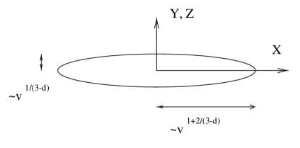
FIG. 1.: Shape of the Larkin domain in the drifting structure. The domain is much longer in directions parralel ($x$) than perpendicular ($y,z$) to ${\bf v}$. Its anisotropy increases with increasing velocity, see Eq. (IV I).

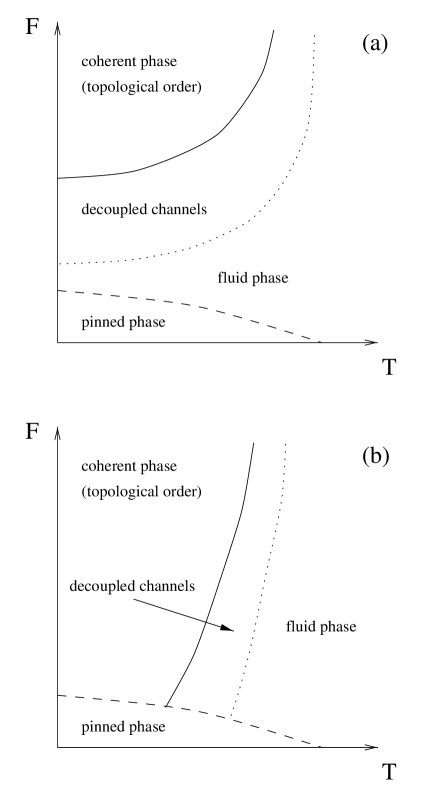
FIG. 2.: Topology of the generic phase diagram of driven periodic media (a) for strong disorder and (b) for weak disorder. At largest velocities the medium moves coherently. At the solid line a melting occurs into an incoherent phase with massive plasticity. This phase can display smectic properties and decay at even smaller velocities (dotted line) into a fluid-like phase. At even smaller velocities (dashed line) the creep phase with metastable states is reached.

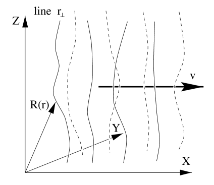
FIG. 3.: Geometry of the vortex lattice in $d=1+2$. Vortices carry a fixed label ${\bf r}_{\perp}$ and their fluctuating position is ${\bf R}$. The $x$-axis is chosen parallel to the average velocity ${\bf v}$.

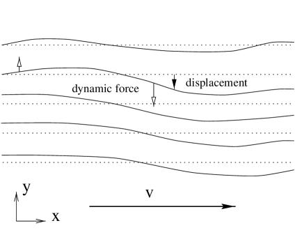
FIG. 4.: Schematic representation of a moving vortex configuration. The distance between the solid wiggly line (position of vortex in perfect lattice) and the dotted straight line (actual vortex position) represents the component $u_{y}$ of the displacements field. The force dynamically generated force $f_{y}\sim\chi_{yyx}\partial_{x}u_{y}$, visualized by empty arrows at two representative positions, makes a vortices acquire the displacement of the preceding vortex.

REFERENCES

- [1] G. Grüner, Rev. Mod. Phys. 60, 1129 (1988).
- [2] D.S. Fisher, Phys. Rev. Lett.50, 1486 (1983); Phys. Rev. B31, 1396 (1985).
- [3] G. Blatter et al., Rev. Mod. Phys. 66, 1125 (1994).
- [4] A.I. Larkin, Sov. Phys. JETP 31, 784 (1970).
- [5] A.I. Larkin and Yu.N. Ovchinnikov, Zh. Eksp. Teor. Fiz. 65 1704 (1973) [Sov. Phys JETP 38 854 (1974)].
- [6] H. Fukuyama and P.A. Lee, Phys. Rev. B 17, 535 (1978).
- [7] A.I. Larkin and Yu.N Ovchinnikov, J. Low Temp. Phys. 34 409 (1979).
- [8] M.V. Feigelman et al., Phys. Rev. Lett. 63, 2303 (1989).
- [9] T. Nattermann, Phys. Rev. Lett. 64, 2454 (1990).
- [10] J.-P. Bouchaud, M. Mézard, and J.S. Yedidia, Phys. Rev. Lett.67, 3840 (1991); Phys. Rev. B 46, 14686 (1992).
- [11] S. E. Korshunov, Phys. Rev. B 48, 3969 (1993).
- [12] T. Giamarchi and P. Le Doussal, Phys. Rev. Lett. 72, 1530 (1994).
- [13] T. Giamarchi and P. Le Doussal, Phys. Rev. B 52, 1242 (1995).
- [14] N.D. Mermin, Phys. Rev. 176, 250 (1968).
- [15] B. Jancovici, Phys. Rev. Lett.19, 20 (1967).
- [16] V.L. Berezinskii, Zh. Eksp. Teor. Fiz. 61, 1144 (1971) [Sov. Phys. JETP 34, 610 (1972)].
- [17] M.P.A. Fisher, Phys. Rev. Lett. 62, 1415 (1989);
- [18] D.S. Fisher, M.P.A. Fisher, and D.A. Huse, Phys. Rev. B 43, 130 (1990).
- [19] J. Kierfeld, T. Nattermann, and T. Hwa, Phys. Rev. B55, 626 (1997); D. Carpentier, P. Le Doussal, and T. Giamarchi, Europhys. Lett. 35, 379 (1996); V. Vinokur et al, preprint 1996; J. Kierfeld, preprint cond-mat/9609045; D. Ertas and D.R. Nelson, Physica C 272, 79 (1996); T. Giamarchi and P. Le Doussal, Phys. Rev. B55, 6577 (1997).
- [20] D.S. Fisher, Phys. Rev. Lett.78, 1964 (1997).
- [21] L.B. Ioffe and V.M. Vinokur, J. Phys. C 20, 6149 (1987).
- [22] T. Nattermann et al. J. Phys. II France 2, 1483 (1992); O. Narayan and D.S. Fisher, Phys. Rev. Lett.68, 3615 (1992); Phys. Rev. B46, 11520 (1992); ibid. 48, 7030 (1993).
- [23] A.A. Middleton, Phys. Rev. Lett.68, 670 (1992).
- [24] Y.-C. Tsai and Y. Shapir, Phys. Rev. Lett. 69, 1773 (1992); Phys. Rev. B 50, 3546 (1994).
- [25] A. E. Koshelev and V.M. Vinokur, Phys. Rev. Lett. 73, 3580 (1994).
- [26] R. Thorel et al., J. Phys. (Paris) 34, 447 (1973).
- [27] S. Bhattacharya and M.J. Higgins, Phys. Rev. Lett.70, 2617 (1993).
- [28] U. Yaron et al., Phys. Rev. Lett.73, 2748 (1994); Nature 376, 753 (1995).
- [29] H.J. Jensen, A. Brass, and A.J. Berlinsky, Phys. Rev. Lett.60, 1676 (1988); A. Brass, H.J. Jensen, and A.J. Berlinsky, Phys. Rev. B39, 102 (1989).
- [30] L. Balents and M.P.A. Fisher, Phys. Rev. Lett.75, 4270 (1995).
- [31] T. Giamarchi and P. Le Doussal, Phys. Rev. Lett.76, 3408 (1996).
- [32] L. Balents, M.C. Marchetti, and L. Radzihovsky, Phys. Rev. Lett.78, 751 (1997).
- [33] T. Giamarchi and P. Le Doussal, preprint cond-mat/9705096.
- [34] A. Schmid and W. Hauger, J. Low Temp. Phys. 11, 667 (1973).
- [35] M. Kardar, G. Parisi, and Y.-C. Zhang, Phys. Rev. Lett.56, 889 (1986).
- [36] P.C. Martin, E.D. Siggia, and H.A. Rose, Phys. Rev. A8, 423 (1973); H.K. Janssen, Z. Phys. B 23, 377 (1976); C. De. Dominicis, J. Phys. C (Paris) 1, 247 (1976).
- [37] R. Bausch, H.K. Janssen, and H. Wagner, Z. Phys. B 24, 113 (1976).
- [38] This cutoff may be chosen in an anisotropic way, e.g. by introducing diffrent cutoffs parallel and perpendicular to the vortices, and . This complication is avoided in the text, but its generalization is straightforward.
- [39] J. Krug, Phys. Rev. Lett.75, 1795 (1995).
- [40] Y.Y. Goldschmidt and B. Schaub, Nucl. Phys. B251, 77 (1985).
- [41] S. Scheidl, Phys. Rev. Lett. 75, 4760 (1995).
- [42] We use the so-called Ito calculus where the instantaneous response vanishes, see appendix C of [37].
- [43] U. Deker and F. Haake, Phys. Rev. A11, 2043 (1975).
- [44] The evaluation of Eq. (107) requires some care. The numerator of the integrand is a difference of two terms. Each term for itself would give rise to a divergence in . This divergence, which is of the same type as in the random force correlator, is canceled in the difference of the two terms.
- [45] L.-W. Chen, L. Balents, M.P.A. Fisher, and M.C. Marchetti, Phys. Rev. B54, 12798 (1996).
- [46] T. Giamarchi and P. Le Doussal, Phys. Rev. Lett.78, 752 (1997).
- [47] H. Sompolinsky and A. Zippelius, Phys. Rev. Lett.47, 359 (1981); Phys. Rev. B25, 6860 (1982).
- [48] H. Kinzelbach and H. Horner, J. Phys. I France 1, 1329 (1993); S. Franz and M. Mézard, Europhys. Lett. 26, 209 (1994).
- [49] D. Ertas and M. Kardar, Phys. Rev. Lett.69, 929 (1992); Phys. Rev. E48, 1228 (1993); Phys. Rev. B53, 3520 (1996).
- [50] T. Hwa, Phys. Rev. Lett.69, 1552 (1992).
- [51] S. Scheidl and V.M. Vinokur, to appear in Phys. Rev. B.
- [52] J.M. Kosterlitz and D.J. Thouless, J. Phys. C 6, 1181 (1973).
- [53] V. Ambegaokar and B.I. Halperin, Phys. Rev. Lett.22, 1364 (1969).
- [54] S.N. Coppersmith, Phys. Rev. Lett.65, 1044 (1990); S.N. Coppersmith and A.J. Millis, Phys. Rev. B44, 7799 (1991).
- [55] L. Balents, M.C. Marchetti, and L. Radzihovsky, preprint cond-mat/9707302.