Attractors in fully asymmetric neural networks

Abstract

The statistical properties of the length of the cycles and of the weights of the attraction basins in fully asymmetric neural networks (i.e. with completely uncorrelated synapses) are computed in the framework of the annealed approximation which we previously introduced for the study of Kauffman networks. Our results show that this model behaves essentially as a Random Map possessing a reversal symmetry. Comparison with numerical results suggests that the approximation could become exact in the large size limit.

¹Dipartimento di Fisica, Università “La Sapienza”, P.le Aldo Moro 2, I-00185 Roma Italy

²HLRZ, Forschungszentrum Jülich, D-52425 Jülich Germany

Keywords: Disordered Systems, Attractor Neural Networks

1 Introduction

In the past decade Attractor Neural Networks were the subject of an intense study as a model of associative memory. The ”ancestor” of these models, the Hopfield model [1], was defined as follows: there is a set of $N$ neurons, each one associated with a binary variable $\sigma_{i}\in\{0,1\},i\in\Omega=\{1,\cdots N\}$, representing its activity. The synaptic couplings between these model neurons, $J_{ij}$, are chosen at random at the beginning and kept fixed, and then the system evolves deterministically according to the equation

$$\sigma_{i}(t+1)={\rm sign}\left(\sum_{j}J_{ij}\sigma_{j}(t)\right)$$ (1)

(parallel updating; alternatively, one can consider sequential updating when $\sigma_{i}(t+1)$ is determined by the state of $\sigma_{j}(t+1)$ for $j<i$ and by $\sigma_{j}(t)$ for $j>i$).

This procedure defines a disordered dynamical system: the evolution is deterministic, but its rules are chosen at random at the beginning and kept fixed. In other words, we can rewrite the dynamic law in the form

$${\cal C}(t+1)=f_{J}\left({\cal C}(t)\right),$$ (2)

where ${\cal C}$ represents a configuration of the system, i.e. a set of values of the $N$ variables $\sigma_{i}$, $f_{J}$ is a random realization of a deterministic map and the set of indices $J$ labels the realization of the dynamic rules.

The most natural distance in configuration space is the normalized Hamming distance, defined as

$$d(C,C^{\prime})={1\over N}\sum_{i}\mid\sigma_{i}-\sigma_{i}^{\prime}\mid.$$ (3)

We are interested in the statistical properties of the motion asymptotically in time and system size. As the motion is deterministic and configuration space is finite, asymptotically in time the dynamics takes place on periodic orbits, and the quantities of interest are the lengths and the number of such orbits as well as the size of their attraction basins. Such quantities are random variables, depending on the realization of the dynamical rules, and we will study their probability distribution.

When the couplings are symmetric ($J_{ij}=J_{ji}$) it is possible to define a Hamiltonian so that equation (1) represents the zero temperature dynamics of a thermodynamic system. In particular, if the $J_{ij}$ are chosen from a distribution with zero mean and variance $1/N$ (for instance a Gaussian distribution) we are dealing with the zero temperature dynamics of the SK model (in the case of sequential updating: the parallel updating does not imply a relaxational dynamics). In the Hopfield model the couplings are symmetric, too, but they are chosen according to the Hebbian rule:

$$J_{ij}=\sum_{\mu=1}^{P}\xi_{i}^{\mu}\xi_{j}^{\mu},$$ (4)

where the $P$ vectors of $N$ binary variables, ${\bf\xi}^{\mu}$, represent the memorized patterns. The system is able to memorize, in the sense that the patterns are fixed points of the dynamics and they are stable against random perturbations if their number does not exceed the capacity of the network, i.e. if $P$ is not larger than $\alpha_{c}N$, with $\alpha_{c}\approx 0.14$. So, given a number of microscopic states growing as $2^{N}$, the Hopfield model is able to memorize a number of patterns growing linearly with $N$.

Asymmetric neural networks received a large attention in the literature in the late ’80s [3, 4, 5, 6, 7, 8]. In 1986 it was proposed to generalize the Hopfield model by taking into account also asymmetric couplings [2].This generalization appears more realistic, since synapses in nature are in general not symmetric, and it suggests a possible way to distinguish between a network that has remembered a learned pattern and a network which is in a confused state (such a distinction is not possible in the Hopfield model). In fact, in asymmetric neural networks, two kind of attractors are present: “ordered” attractors, that are either short cycles or fixed points, and “chaotic” attractors, whose length grows exponentially with system size. The first numerical observations of this twofold nature of the attractors are due to Gutfreund, Reger and Young [5] and to Nützel [9].

In this note we are mainly interested in the study of the properties of the attractors, such as the probability distributions of their lengths, of their number and of the size of their attraction basins. We will consider only the case of fully asymmetric couplings, i.e. $J_{ij}$ and $J_{ji}$ are independent random variables. In this case analytical results have already been obtained about the correlation functions [6, 7] and about the number of attractors [11], but more about the attractors can be said using a simple stochastic scheme based on the annealed approximation. This approximation was introduced in the study of disordered dynamical systems by Derrida and Pomeau [12] to study damage spreading in Kauffman networks (a disordered dynamical system proposed as a model of the genetic regulation in cells [13]). In [14] we showed that it can also be used to obtain information about the attractors of that model.

A reason of interest of this study is that asymmetric neural networks are the limit case of a one parameter family of models, the parameter $\eta$ representing the symmetry of the synaptic couplings:

$$\eta={\left\langle J_{ij}J_{ji}\right\rangle\over\left\langle J_{ij}\right\rangle^{2}}.$$ (5)

The case $\eta=0$ represents the present model (fully asymmetric couplings), while for $\eta=1$ the couplings are fully symmetric and we obtain the mean field model of spin glasses. Thus the parameter $\eta$ connects with continuity asymmetric neural networks to a disordered system of statistical mechanics.

It was suggested through numerical simulations that the model with generic correlation undergoes a dynamical transition when $\eta$ is changed [9, 10, 15]. The transition seems to take place when the absolute value of $\eta$ crosses the value $1/2$. For $|\eta|<1/2$ the dynamics is chaotic and the typical length of the cycles increases exponentially with the number of neurons $N$, while for $|\eta|>1/2$ the dynamics is frozen and the typical length of the cycles does not increase with system size (most of the cycles have length 2, for positive $\eta$, and 4 for negative $\eta$).

This transition is reminiscent of the dynamical transition taking place in Kauffman networks. Also in that case the typical length of the cycles grows exponentially with $N$ in the so called chaotic phase, remains finite in the frozen phase and grows less than exponentially with $N$ on the critical line [13, 14]. It was claimed by Kauffman that the critical line of his model can be a good model of the genetic regulatory systems acting in cell differentiation, thus showing that such systems do not need to be tuned in the very details by natural selection but behave similarly to typical realizations of an ensemble of random regulatory networks [13]. It is possible that, analogously, also the supposed critical point in attractor neural networks, where chaotic and ordered cycles coexist, can suggest something interesting from a biological point of view. We think that our method can be modified to give information about systems with generic asymmetry and about the supposed phase transition that they undergo, though this probably requires to go beyond the annealed approximation.

2 Closing probabilities

2.1 General framework

Our strategy for the study of attractors in disordered dynamical systems has as starting point the probability distribution of the distance at different time steps. Actually, the information contained in the distribution of the distance is much more than what we need and this distribution is in principle a very complicated object, so that our approach may seem to complicate the problem. But, in some cases, the distance can be well approximated by a suitably defined stochastic process and the computation becomes much easier. The simplest possibility is to approximate the distance with a Markovian stochastic process. This is what we call here the annealed approximation.

An apparently paradoxical aspect of this approach is that in disordered dynamical systems attractors exist due to the fact that the motion is deterministic. Stochastic processes, on the other hand, have nothing similar to a limit cycle. Nevertheless, all the properties of the attractors can be derived from the distribution of distances, which is a well defined object in both kinds of models. We can not pursue this analogy up to times larger than the time of first recurrence of a configuration already visited, when the deterministic motion becomes periodic. But this is enough, since the first recurrence provides us with every information about the length of the cycles and the transient time.

The fundamental object of our study will be then the distribution of distances between configurations at time steps $t$ and $t^{\prime}>t$ on the same trajectory, restricted to trajectories that have not yet visited twice any configuration up to the larger time $t^{\prime}$ (thus the effects of periodicity do not yet appear). We will call this condition the opening condition, and denote it by the symbol $A_{t^{\prime}}$. The closing probability $\pi_{N}(t,t^{\prime})$ is the probability that configurations at time steps $t$ and $t^{\prime}$ are equal ($d(t,t^{\prime})=0$), subject to the opening condition:

$$\pi_{N}(t,t^{\prime})=\Pr\left\{d(t,t^{\prime})=0\mid A_{t^{\prime}}\right\}$$ (6)

(the subscript $N$ is there to remember the dependence on system size).

After the closing time $t^{\prime}$ the trajectory enters a periodic orbit of length $l=t^{\prime}-t$, where $t$ is the transient time. In terms of the closing probabilities, the probability to find such a trajectory is easily computed. First we have to know the probability $F_{N}(t)$ that the trajectory was not closed before time $t^{\prime}=t+l$. This obeys the equation $F_{N}(t+1)=F_{N}(t)\left(1-\sum_{t^{\prime}=0}^{t-1}\pi_{N}(t^{\prime},t)\right)$, whence, introducing a continuous time variable, we get

$$F_{N}(t)=\exp\left(-\int_{0}^{t}dt^{\prime}\int_{0}^{t^{\prime}}dt^{{}^{\prime\prime}}\pi_{N}(t^{\prime},t^{{}^{\prime\prime}})\right)$$ (7)

(to have a slightly simpler formula we made the hypothesis that the typical closing times are long, which is normally the case in the chaotic phase, where they grow exponentially with system size $N$, and we transformed the sum into an integral).

The probability to find a trajectory that, after a transient time $t$, enters a cycle of length $l$ is then obtained multiplying $F_{N}(t+l)$ times the closing probability $\pi_{N}(t,t+l)$.

2.2 The annealed approximation

Regarding the distance as a Markovian stochastic process is a very drastic approximation. In our case it sounds reasonable when the temporal distance $l$ is large, since the model that we study is known to have a behavior very reminiscent of chaos [15]. However in this way we neglect some memory effects, which can play a fundamental role in systems with nonzero symmetry.

This approximation was first used in this context by Derrida and Pomeau [12], who studied the damage spreading in Kauffman networks. They showed that the average value of the Hamming distance between two different trajectories is equivalent, in the infinite system limit, to the average value of the Markovian stochastic process obtained extracting new dynamical rules at every time step and keeping memory only of the value of the distance at time step $t-1$. Thus the disorder is treated as annealed rather than as quenched. In other words, instead of considering an ensemble of trajectories, each one taking place on a fixed realization of the dynamical rules, they consider an ensemble of trajectories moving from one realization of the dynamical rules to another one, in the same spirit in which the annealed average is used for disordered thermodynamical systems.

The above procedure can be shown to describe exactly the evolution of the average distance up to time of order $\log N$ in disordered systems with finite connectivity [16, 17], but we think that its validity is more general. In systems with infinite connectivity like the one that we are studying here, or when one is interested in the whole distribution of the distance, the equivalence between the two dynamics has not been proved, and we have to assume that a typical trajectory of the quenched system loses memory of the details of the realization of dynamical rules under which it evolves. In the Random Map model [18] this is trivially true. In other cases this can be thought of as a maximal ignorance hypothesis, whose consequences must then be compared with numerical simulations.

Let us state some of these consequences. A Markovian stochastic process, if its transition probability is ergodic, converges to a stationary stochastic variable independent of the initial distribution. This means that the closing probability $\pi_{N}(t,t+l)$ converges to a stationary value $\pi_{N}^{*}$. This is also independent of $l$ if the transition probability does not depend on this quantity. We will show that this happens in the present case, at least for $l$ large enough.

It is then easy to compute the probability of a trajectory which, after a transient time $t$, enters a cycle of length $l$ (with $l$ and $t$ large enough, so that the closing probability has reached its asymptotic value): using the results of last section, we get

$$\Pr\left\{T=t,L=l\right\}={1\over\tau^{2}_{N}}\exp\left(-{1\over 2}\left({t+l\over\tau_{N}}\right)^{2}\right),$$ (8)

where $\tau_{N}={\pi^{*}_{N}}^{-1/2}$ is the typical time scale of the problem, in the sense that the random variable $t/\tau_{N}$ has a well defined density of probability even in the limit where $\tau$ goes to infinity. All the dependence on system size is contained into the factor $\pi^{*}_{N}$, which is expected to decrease exponentially with $N$ in the chaotic phase. For instance, for a uniform Random Map [18], which is the most chaotic disordered dynamical system, it holds $\pi^{*}_{N}=1/2^{N}$, and consequently the typical time scale of the attractors grows as $2^{N/2}$.

The properties of Random Maps can be easily generalized starting from equation (8). An interesting quantity is the distribution of the attraction basin weights. This was analytically computed by Derrida and Flyvbjerg for the case of the uniform RM [19]. The weight of the attraction basin of cycle $\alpha$, $W_{\alpha}$, is defined as the probability to extract at random an initial configuration which will reach asymptotically the attractor $\alpha$. The statistical information about the distribution of the weights can be expressed through the “moments” $\langle Y_{n}\rangle$, defined as

$$\left\langle Y_{n}\right\rangle=\sum_{\alpha}\left\langle W_{\alpha}^{n}\right\rangle.$$ (9)

$Y_{1}$ is equal to 1 due to the normalization of the weights and $Y_{2}$ represents the average weight in a given dynamical system. Its extreme values, 1 and 0, correspond respectively to the “ergodic” case where there is only one relevant attractor and to the case where there is an infinite number of relevant attractors, while a finite value of $Y_{2}$ means that there is a finite number of attractors with non vanishing weight. This quantity fluctuates from sample to sample, so it is necessary to consider an average over the realizations of the dynamical rules, that is represented by the angular brackets.

The method used in [19] to compute the distribution of the weight can be applied without modifications to all disordered dynamical systems where the closing probability reaches an asymptotic value, $\pi^{*}_{N}$, and the result do not depend on this value in the large size limit. Thus the distribution of the attraction basin weights is universal for all the disordered dynamical systems where the closing probability reaches a stationary value [14, 21], apart for systems which possess some symmetry. The result for the average value of the $Y_{n}$ is [19]

$$\langle Y_{n}\rangle={4^{n-1}\left[(n-1)!\right]^{2}\over(2n-1)!}.$$ (10)

The fluctuations from sample to sample can also be computed. For example the fluctuations of $Y_{2}$ are measured by $\langle Y^{2}_{2}\rangle-\langle Y_{2}\rangle^{2}$, and do not cancel even in the infinite size limit $N\rightarrow\infty$.

The average number of attractors of length $l$ can be computed starting with the relation

$$\left\langle n_{a}(l)\right\rangle={2^{N}\over l}\Pr\{T=0,L=l\}.$$ (11)

In this formula, the probability $\Pr\{L=l,T=0\}$ should be computed multiplying $F_{N}(l)$, given in equation (7), times the closing probability $\pi_{N}(0,l)$. This is different from the asymptotic value (for large $t$) of $\pi_{N}(t,t+l)$. According to the hypothesis, on which the annealed approximation relies, that the system is going to lose memory of the details of the evolution, we expect no correlations between the initial configuration and a configuration at a large time $l$ or, in other words, we expect the closing probability to be, asymptotically in $l$, $\pi_{N}(0,l)=1/2^{N}$. For chaotic Kauffman networks this can be explicitly computed in the framework of the annealed approximation, which is then consistent under this point of view. Moreover, we find in this case $\pi_{N}(0,l)=c_{l}1/2^{N}$, where $c_{l}$ does not depend on $N$. Thus it holds

$$\left\langle n_{a}(l)\right\rangle\approx{c_{l}\over l}\exp\left(-l^{2}/2\tau^{2}\right).$$ (12)

Summing over $l$ we obtain the average value of the total number of cycles, whose leading term in $N$ is equal to $\log\tau_{N}$. Since in the chaotic phase the time scale grows exponentially with system size, the number of attractors is proportional to $N$ in this case. This computation holds for chaotic Kauffman networks in the framework of the annealed approximation, but we expect it to hold more generally under the hypothesis discussed above.

2.3 Master equation

The general scheme described above must be modified in the case studied in this note, to take into account the symmetry of the problem. Let us define the reversal operator, $R$, which reverses all the spins. This operator commutes with the dynamics of the system. Using the notation defined in equation (2), we can write:

$$f_{J}\left(R{\cal C}\right)=Rf_{J}\left({\cal C}\right),$$ (13)

This implies that we can define two different closing times:

1. The first time $t$ when ${\cal C}(t)$ is equal to ${\cal C}(t+l)$.

2. The first time when ${\cal C}(t+l)$ is equal to $R{\cal C}(t)$: then equation (13) implies ${\cal C}(t+2l)={\cal C}(t)$. In other words, the trajectory has reached, after a transient time $t$, a cycle of length $2l$.

These closing events can be described in terms of the Hamming distance between configurations: the first one corresponds to $d(t,t+l)=0$, while the second one corresponds to $d(t,t+l)=1$. Thus two closing probabilities must be defined:

$$\pi_{N}^{(0)}(t,t^{\prime})=\Pr\left\{d(t,t^{\prime})=0\mid A_{t^{\prime}}\right\},$$ (14)

$$\pi_{N}^{(1)}(t,t^{\prime})=\Pr\left\{d(t,t^{\prime})=1\mid A_{t^{\prime}}\right\},$$ (15)

and the opening condition, $A_{t}$, has the meaning that up to time $t$ it never occurred either $d(t_{1},t_{2})=0$ or $d(t_{1},t_{2})=1$. Our task is now to compute the master equation for the distribution of the distance under the opening condition (this means that we consider only trajectories not yet closed) and under the hypothesis that the distribution of $d(t+1,t^{\prime}+1)$ depends only on the distribution of $d(t,t^{\prime})$. This is not a difficult task. To simplify slightly the formulas we will consider, instead of the distance, the overlap $q=1-d$, which is measured by the number of elements whose state is the same in the two configurations, divided by $N$.

An element $\sigma_{i}$ is in the same state at time $t+1$ and $t^{\prime}+1$ if its local field has the same sign at time steps $t$ and $t^{\prime}$. Thus it holds

$$\sigma_{i}(t+1)\sigma_{i}(t^{\prime}+1)={\rm sign}\left(\sum_{jk}J_{ij}J_{ik}\sigma_{k}(t)\sigma_{j}(t^{\prime})\right).$$ (16)

Let us consider separately the contribution to this sum coming from the spins whose state is the same at time steps $t$ and $t^{\prime}$, whose number is $Nq(t,t^{\prime})$, and that belong to a set that we indicate with the name $I(t,t^{\prime})$. We can then write

$$\sigma_{i}(t+1)\sigma_{i}(t^{\prime}+1)={\rm sign}\left((h_{i}^{+}(t))^{2}-(h_{i}^{-}(t))^{2}\right),$$ (17)

where

$$h_{i}^{+}(t)=\sum_{j\in I(t,t^{\prime})}J_{ij}\sigma_{j}(t),$$ (18)

$$h_{i}^{-}(t)=\sum_{j\in\Omega/I(t,t^{\prime}))}J_{ij}\sigma_{j}(t).$$

The annealed approximation consists in considering the local fields as random variables, correlated to the previous story of the system only through the value of $q(t,t^{\prime})$. In this spirit, we consider a dynamics in which the local fields are extracted at random at every time step, under the following assumptions:

1. The local fields at different points are independent random variables;

2. The value of $\sigma_{j}(t)$ is independent on the synaptic coupling $J_{ij}$.

Both these assumptions have troubles when the synaptic couplings are correlated with each other, but they are quite reasonable for $\eta=0$, which is the case that we are studying now. Assumption 1 implies that the transition probability is a binomial one:

$$\Pr\left\{q(t+1,t^{\prime}+1)=q_{n}\mid q(t,t^{\prime})=q_{m}\right\}={N\choose n}\left(\gamma(q_{m})\right)^{n}\left(1-\gamma(q_{m})\right)^{N-n},$$ (19)

where $q_{n}=n/N$, and $\gamma(q)$ is the probability that $|\tilde{h}^{+}(q)|>|\tilde{h}^{-}(1-q)|$, where, following assumption 2, $\tilde{h}^{\pm}(q)$ is a Gaussian variable with mean value zero and variance $q$ (this result is independent on the details of the distribution of the couplings, provided that they are all independent variables with mean value zero and with the same variance). A straightforward computation shows that

$$\gamma(q)={2\over\pi}\arcsin\sqrt{q}.$$ (20)

The Markov process associated to this transition probability is ergodic if we exclude as starting points the values $q=0$ and $q=1$, as we do imposing the opening condition, and the distribution of the distance evolves towards a stationary distribution. Moreover, since the transition probability is independent on $l=t^{\prime}-t$, also the stationary distribution is independent on $l$, which appears only in the initial distribution of the variable $q(0,l)$. It is also evident from the symmetry of the problem that it must hold $\gamma(q)=1-\gamma(1-q)$, so, if also the initial distribution is symmetric (e.g. a binomial distribution around $q=1/2$), the overlap distribution will be symmetric at every time step and it will be concentrated around the value $Q(t,t^{\prime})=D(t,t^{\prime})=1/2$ (the distributions of the overlap and of the distance are perfectly equivalent in this case). The stationary distribution is, independently on the initial one, concentrated around the value $Q^{*}$ solution of the self-consistent equation:

$$Q^{*}=\gamma\left(Q^{*}\right)={2\over\pi}\arcsin\sqrt{Q^{*}}.$$ (21)

This equation has three solutions: $1/2$, 1 and 0, but only the first one can be accepted, according to the criterion $|\gamma^{\prime}(Q^{*})|<1$, which can be obtained either as the stability condition of the fixed point $Q^{*}$ of the map $Q(t+1,t^{\prime}+1)=\gamma(Q(t,t^{\prime}))$, or as the condition that the variance of the stationary distribution is positive (see equation (25) below).

Equation (21) is equivalent to the equation for the stationary value of the correlation function rigorously derived in [6] through a functional integral approach, so that one can see from this comparison that the annealed approximation gives an exact (though trivial) result concerning the average overlap. But our task here is to compute the whole stationary distribution of the overlap, and we can not prove that the annealed approximation is correct to this extent, so we have to rely upon simulations to control its validity.

Though it is concentrated around $Q^{*}=1/2$, the stationary distribution is much broader than a binomial one and thus the closing probability is exponentially larger than $1/2^{N}$. In order to compute its value, we proceed in this way [14]: since the transition probability is exponentially concentrated, we look for a solution of the form:

$$P_{N}\left(q(t,t^{\prime})=q_{n}\right)=C_{N}(q_{n},t)\exp\left(-N\alpha_{t}(q_{n})\right),$$ (22)

where we have dropped the $l$ dependence of the probability, which disappears at stationarity. Using Stirling approximation for the binomial coefficient and the saddle point approximation to average over the distribution at time step $t-1$, we get the following equation for the evolution of the exponent of the distribution, $\alpha_{t}(x)$:

$$\alpha_{t}(x)=\alpha_{t-1}(q_{t}(x))+x\log\left({x\over\gamma(q_{t}(x))}\right)+(1-x)\log\left({1-x\over 1-\gamma(q_{t}(x))}\right),$$ (23)

where the function $q_{t}(x)$ must be determined self consistently solving the equation

$$\alpha^{\prime}_{t-1}(q_{t}(x))-\gamma^{\prime}(q_{t}(x))\left({x\over\gamma(q_{t}(x))}-{1-x\over 1-\gamma(q_{t}(x))}\right),$$ (24)

with the conditions $q_{t}(x)>0$ and $q_{t}(x)<1$.

At stationarity the most probable overlap (the point where $\alpha_{t}(q)$ has a minimum) is given by equation (21), and the variance of the distribution can be obtained taking the second derivative of equation (23) and solving it together with the first derivative of the saddle point condition (24). The result is

$$V^{*}={Q^{*}\left(1-Q^{*}\right)\over 1-\left(\gamma^{\prime}(Q^{*})\right)^{2}}={1/4\over 1-(2/\pi)^{2}}\approx 0.4204,$$ (25)

where $V^{*}$ is the variance of the stationary distribution multiplied times $N$. Thus the variance is larger than in the case of a binomial distribution, since the dynamics has produced correlations between different elements.

The value of the closing probability can not be computed analytically: we need for this the whole function $\alpha(x)$, and to obtain it we should solve a transcendent non local equation. Thus we had to solve numerically equation (23), obtaining the stationary distribution reported in Figure 1. The asymptotic closing probability, defined as $P_{N}^{*}(q=1)+P_{N}^{*}(q=0)$, is thus

$$\pi^{*}_{N}=2\exp\left(\alpha N\right),$$ (26)

with $\alpha=0.4554$. As discussed in the previous section, the exponent of the average length of the cycles should be equal to $\alpha/2$. This prediction is in good agreement with the numerical simulations that will be reported in section 4.

2.4 Initial distribution

In order to compute the average number of cycles we have to know the distribution of the overlap with the initial configuration, $q(0,l)$, which plays the role of the initial distribution for the stochastic process studied in the previous subsection. Although the number of cycles in fully asymmetric neural networks was already exactly studied by Schreckenberg [11], we want to sketch the annealed computation of it, since it is much simpler and it can be generalized to more complex situations.

Our aim is to compute the distribution of $q(0,l)$. After one time step the annealed approximation is exact (we have still to extract all the couplings) and trivial: every spin can be either in its initial state or in the reversed one with probability 1/2, and the overlap $q(0,1)$ multiplied times $N$ has a binomial distribution with $p=1/2$. After two time steps we distinguish two contributions in the local field: one coming from the set $I_{1}$ of the spins which are in the same state at $t=0$ and at $t=1$ and another one coming from all the other spins. We write

$$\sigma_{i}(0)\sigma_{i}(2)={\rm sign}\left(\sum_{j\in I_{1}}\sigma_{i}(0)J_{ij}\sigma_{j}(0)-\sum_{j\in\Omega/I_{1}}\sigma_{i}(0)J_{ij}\sigma_{j}(0)\right).$$ (27)

Since the states $\sigma_{i}(0)$ and $\sigma_{j}(0)$ are independent both one on each other and on the couplings, we can set them equal to 1. If we change the sign of the last sum, we obtain $\sigma_{i}(0)\sigma_{i}(1)$. Thus, depending on whether this is positive or negative, there are two possibilities:

$$\sigma_{i}(0)\sigma_{i}(2)=\left\{\begin{array}[]{lr}{\rm sign}\left(\left(\sum_{j\in I_{1}}J_{ij}\right)^{2}-\left(\sum_{j\in\Omega/I_{1}}J_{ij}\right)^{2}\right),&if\;\sigma_{i}(0)\sigma_{i}(1)>0\\ {\rm sign}\left(\left(\sum_{j\in\Omega/I_{1}}J_{ij}\right)^{2}-\left(\sum_{j\in I_{1}}J_{ij}\right)^{2}\right),&if\;\sigma_{i}(0)\sigma_{i}(1)<0\end{array}\right.$$ (28)

(there is indeed in this formula a small imprecision, which becomes negligible in the infinite size limit: since the coupling $J_{ii}$ is set equal to zero, we have not to take into account the spin $j=i$ itself, which contributes to the first sum in both lines). The probability that the sum of $n$ Gaussian variables has a module larger than that of the sum of $N-n$ other Gaussian variables was already computed in the previous section, where it received the name $\gamma(n/N)$. Taking all this into account, we come to the transition probability

$$\Pr\left\{q(0,2)=m/N\mid q(0,1)=n/N\right\}=$$ (29)

$$\hskip 56.9055pt=\sum_{k}{n\choose k}{N-n\choose m-k}\left(\gamma(n/N)\right)^{N-n-m+2k}\left(1-\gamma(n/N)\right)^{n+m-2k},$$

where, as usual, the opening condition imposes to exclude as starting points $n=0$ and $n=N$, and the sum runs over all the values of $k$ for which the factorial is well defined. The closing probability which can be deduced from this formula setting either $m=N$ or $m=0$ coincides with the one exactly computed in ref. [11]. It can be easily seen that it is proportional to $1/2^{N}$, as expected (the system loses memory of the initial configuration quite fast), and the proportionality coefficient can be computed with the saddle point method [11]

In the general case, the information about $q(0,l)$ is not enough to compute the distribution of $q(0,l+1)$: we have also to know the value of $q(0,1)$, as it can be seen from equation (28) where we have to substitute 1 with $l$ and 2 with $l+1$ in the equations but we have to keep memory of $\sigma_{i}(0)\sigma_{i}(1)$ in the conditions. In the general case the transition probability has thus the form

$$\Pr\left\{q(0,l+1)=m/N\mid q(0,1)=n_{1}/N,q(0,l)=n/N\right\}=$$ (30)

$$\hskip 56.9055pt=\sum_{k}{n_{1}\choose k}{N-n_{1}\choose m-k}\left(\gamma(n/N)\right)^{N-n_{1}-m+2k}\left(1-\gamma(n/N)\right)^{n_{1}+m-2k},$$

and we have to consider the evolution of the joint distribution of the variables $q(0,1)$ and $q(0,l)$. As expected, the correlations between these two variables vanish very fast as $l$ grows, and the stationary distribution is the product of two binomial distributions, as it can be easily checked, so that for large $l$ the closing probability is $\pi_{N}^{(a)}(0,l)=1/2^{N}$ (with $a$ equal either to 1 or to 0), consistently with the supposed loss of memory and in agreement with the exact results of ref [11]. For small values of $l$ it can be seen that $\pi_{N}^{(a)}(0,l)=c_{l}/2^{N}$, where $c_{l}$ goes to a finite value in the infinite size limit, so that the total number of cycles increases only proportionally to system size.

3 Reversal symmetry

The computations shown in section 2.2 must be modified to take into account the twofold nature of the closing probability. We have to distinguish between two kinds of cycles, with different properties under the reversal operation:

1. Cycles that close when ${\cal C}(t+l)=R{\cal C}(t)$ (or, in other words, $q(t,t+l)=0$), whose length is $2l$. They are invariant under the reversal operation: each configuration is present together with its reversed one.

2. Cycles that close when $q(t,t+l)=1$. In this case the reversal operator applied to the cycle $\Gamma$ produces a new cycle $R\Gamma$ with equal length and equally large attraction basin.

Taking this into account, we have to distinguish between cycles of even length, which can be of one of the two kinds, and cycles of odd length, which can be only of the first kind. Cycle length distribution is then

$$\Pr\left\{T=t,L=l\right\} ={1\over 2\tau^{2}}\exp\left(-{(t+l)^{2}\over 2\tau^{2}}\right),\;l\>\>{\rm odd};$$ (32)

$$={1\over 2\tau^{2}}\exp\left(-{(t+l)^{2}\over 2\tau^{2}}\right)+{1\over 2\tau^{2}}\exp\left(-{(t+l/2)^{2}\over 2\tau^{2}}\right),\;l\>\>{\rm even},$$

with $\tau=1/\sqrt{\pi}^{*}=1/\sqrt{2}\exp(0.2277N)$.

The cycles of the first type have only even length, so that their number is half of the number of the cycles of the second type. Using the result of subsection 2.2 and summing up the contributions of both types of cycles we obtain, at the leading order in $N$,

$$\sum_{l}\langle n_{a}(l)\rangle\approx{3\over 2}\log\tau={3\over 4}\alpha N,$$ (33)

which is $3/2$ times larger than in a Random Map with the same closing probability.

The most important difference between attractors in Asymmetric Neural Networks and in a Random Map involves the distribution of the attraction basins weights. Let us consider separately cycles of the first type and cycles of the second type (taking only one cycle to represent each pair of cycles of the second type). We then get the expression of the moments $\langle Y_{n}\rangle$ of the distribution of the weights:

$$\langle Y_{n}\rangle={1\over 2}\left\langle\sum_{\alpha^{\prime}}W_{\alpha^{\prime}}^{n}+2\sum_{\alpha^{{}^{\prime\prime}}}\left(W_{\alpha^{{}^{\prime\prime}}}/2\right)^{n}\right\rangle,$$ (34)

where the sum over $\alpha^{\prime}$ and $\alpha^{{}^{\prime\prime}}$ of the weights are both normalized to one. Under the hypothesis that each of the two sets of weights is distributed as in a Random Map, we get

$$\langle Y_{n}\rangle=\left({1\over 2}+{1\over 2^{n}}\right)\langle Y_{n}\rangle_{RM},$$ (35)

or, using (10),

$$\left\langle Y_{n+1}\right\rangle={1\over 2}{\left(n!\right)^{2}\over\left(2n+1\right)!}\left(4^{n}+2^{n}\right).$$ (36)

Thus the moments of the distribution of the weights are smaller than in the usual Random Map, for instance $\langle Y_{2}\rangle=1/2$ instead of 2/3. These results are in very good agreement with numerical simulations.

To prove equation (35) let us recall that $\langle Y_{n}\rangle$ can be interpreted as the probability that $n$ randomly chosen trajectories reach the same attractor. We can compute such quantity using the closing probabilities and following exactly the same lines as in [19], but we have to remember that a closing event has two different meanings: either a closure on an identical configuration ($q=1$) or a closure on a reversed configuration ($q=0$). Thus not all the events which represent the closure of the $n$ trajectories, and whose probability is exactly $\langle Y_{n}\rangle_{RM}$, have the meaning that the trajectories will ultimately meet. If the first trajectory closes with $q=0$ (this happens with probability 1/2), its attraction basin contains also all of the reversed configurations, and the following $n-1$ trajectories which close on it will then go to the same attractor, regardless on how they close. On the contrary, if the first trajectory closes with $q=1$, the following $n-1$ trajectories have also to close with $q=1$ in order to go to the same attraction basin (if they close with $q=0$, they go to the reversed basin). In this case, whose probability is again $1/2$, a closing event is equivalent to an asymptotic meeting of the $n$ trajectories only with probability $1/2^{n-1}$. Equation (35) is thus proved.

3.1 Explicit symmetry breaking

The above picture of the distribution of the attraction basins weights is completely destroyed by the introduction of a magnetic field, however small, in the equations of motion (1), which restores the distribution typical of a Random Map. We considered the dynamic rules

$$\sigma_{i}(t+1)={\rm sign}\left(\sum_{j}J_{ij}\sigma_{j}(t)-h\right)$$ (37)

The magnetic field $h$ has the biological meaning of the threshold of activation of the neurons. In real neurons, such non-zero threshold exists and can be different from one neuron to another one. In our simplified model, we take a threshold which is constant among the different neurons. Its introduction explicitly breaks the symmetry respect to the reversal of all the neural activities.

In the framework of the annealed approximation, the conditional probability that the activity of a neuron is the same in two different time steps is not more symmetric, i.e. $\gamma(1-q)$ is different from $1-\gamma(q)$ and $\gamma(1)$ increases very fast respect to the above case, thus making very unlikely a reversed closure, while $\gamma(0)$ decreases. After a straightforward calculation we get

$$\gamma(q)=1-{2\over\pi}\int_{\rm arcsin\sqrt{q}}^{\pi/2}\exp\left(-{1\over 2}\left(h/\sin t\right)^{2}\right)dt.$$ (38)

For large threshold the closing probability differs from 1 by a value that cancels very fast, as $\exp\left(-h^{2}/2\right)$.

The attractors of the first type (such that $\Gamma=R\Gamma$) are completely destroyed in this way, while attractors of the second type do not live in pairs anymore, and the distribution of the weights is of the Random Map type.

4 Numerical results

4.1 Distribution of the overlap and closing probabilities

Our first aim was to compare the distribution of the overlap predicted by the annealed approximation with the same distribution in the quenched system. As we wrote, the analogy holds if we measure the overlap between configurations only along the trajectories that are not yet closed when we do the measurement. Under this condition, we computed the distribution of the overlap $q(t,t+l)$ for $l$ fixed and $t$ large enough to suppose that the distribution has attained stationarity.

The exponent $\alpha(q)$ of the distribution of the overlap is defined by the equation $P_{N}(q)=C_{N}(q)\exp\left(-N\alpha(q)\right)$, where the factor $C_{N}(q)$, proportional to $1/\sqrt{N}$, comes from the Stirling expansion of the binomial coefficient. Thus we computed $\alpha(q)$ using the formula

$$\alpha(q)=-{1\over N}\left(\log\left(P_{N}(q)\right)+{1\over 2}\log N\right).$$ (39)

The logarithmic term must not be subtracted when $q$ is equal to 0 or 1, because in this case the $1/\sqrt{N}$ factor is no more present in the expansion of the binomial coefficient, and so we did not consider it for $q=0$ and 1, interpolating linearly between the two formulas for values of $q$ between 0 and $0.1$ and between $0.9$ and 1. In such data analysis we neglect terms of order $1/N$ (there is also an unknown coefficient in the expression of the probability $P(q)$), and the agreement between the annealed prediction for $\alpha(q)$ and the quenched data, compared in Figure 1, is then very satisfactory even for a system of such a small size (we considered $N=20$). When $l$, the temporal distance between configurations, is small, there are some discrepancies (for instance, for $l=2$ the quenched distribution is much broader than expected, and the closing probability is consequently much higher), but when $l$ is large the agreement improves (in particular, the variance of the distribution and the exponents $\alpha(0)$ and $\alpha(1)$ of the closing probabilities coincide within the errors with the predicted values). This fact sustains our interpretation that the annealed approximation is valid when the temporal distance is large, so that the system has lost memory of the details of its evolution [14, 21].

Figure 1: Exponent $\alpha(q)$ computed from the equation $P_{N}(q)=C_{N}(q)\exp\left(-N\alpha(q)\right)$, where $P_{N}(q)$ is the stationary overlap distribution, with both $q=q(t,t+2)$ (diamonds) and $q=q(t,t+32)$ (triangles). The solid line shows the annealed prediction. The agreement is better in the second case, when the temporal distance between configurations is larger. System size is $N=20$ and $h=0$.

Next we measured the closing probability $\pi_{N}(t,t+l)$. Figure 2 represents this quantity as a function of $t$ for different values of $l$, kept fixed. The statistic errors are large, but it appears that $\pi(t,t+l)$ reaches a value approximately stationary in $t$, in agreement with the annealed prediction, when $l$ is large (in figure 2b we have $l=11$) but when $l$ is small (in figure 2a $l=2$) the closing probability reaches a maximum value and then decreases, as a function of $t$. We already observed this kind of non monotonic behavior of the closing probabilities in simulations of Kauffman model. In both cases we interpret the decreasing part of $\pi(t)$ as due to the opening condition: the condition that the trajectory is not closed up to time $t$ selects, as $t$ grows, trajectories which are more and more unlikely to close. The opening condition cannot be imposed in the annealed scheme, because we consider the stochastic process $d(t,t+l)$ with $l$ fixed and we cannot control $d(t,t^{\prime})$ for generic $t$ and $t^{\prime}$. So the annealed scheme must be modified to take into account this fact [14]. But in asymmetric neural networks, differently from what we observed in Kauffman networks, the opening condition seems to be irrelevant when the temporal distance $l$ is large, and the closing probability appears to reach in this case an approximately stationary value.

Figure 2: Closing probability $\pi_{N}(t,t+l)$ as a function of $t$, for $l=2$ (a) and $l=11$ (b). System size is $N=20$ with $h=0$.

The non-stationarity of the distribution of $q(t,t+2)$ shows the existence of memory effects in the model: the statistical properties of $q(t,t+2)$ still depend on $t$, even after an arbitrarily long transient time. It would be interesting to find out whether the lack of time translation invariance in the system with completely uncorrelated couplings has some relation with aging in the relaxational dynamics of the SK spin glass model [22]. In the present case, however, the lack of time translation invariance is only a minor effect and does not prevent the overlap $q(t,t+l)$ from reaching a stationary distribution for $l$ large enough. The macroscopic properties of the dynamics can be predicted, in good agreement with numerical results, also neglecting this effect at all.

We conclude this subsection showing a plot of the integral closing probability $\tilde{\pi}_{N}(t)$, defined as

$$\tilde{\pi}_{N}(t)=\sum_{t^{\prime}=0}^{t-1}\pi_{N}(t^{\prime},t)$$ (40)

this is the probability that a trajectory not closed at time $t-1$ closes at time $t$). In Kauffman networks, this quantity is non-monotonic as a function of $t$: it increases to a maximum value and then decreases with $t$. On the other hand, from the annealed approximation we would expect it to increase linearly with $t$ in the stationary state. In asymmetric neural networks we found that the integral closing probability increases monotonically with $t$. After a transient phase of very fast increase it slows down, and asymptotically it appears to behave as a power law. For the largest systems that we simulated our data are very noisy, and we could fit the asymptotic $t$ behavior only for $N=20$, finding that the best fit exponent of the power law is approximately $0.6$. So, at least for systems of not very large size, deviations from the annealed approximation are present also in this case.

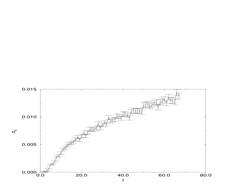
Figure 3: Integral closing probability, $\pi_{N}(t)=\sum_{t^{\prime}}\pi_{N}(t^{\prime},t)$ as a function of $t$ in a system of size 20 with $h=0$

4.2 Properties of attractors: zero threshold

To obtain the first three moments of the distribution of the attraction basins we followed the method indicated in [20]. For every value of the parameters $N$ and $h=0$ we generated at random 2000 networks, extracting the synaptic couplings with Gaussian distribution, and we simulated four randomly chosen trajectories on each of them.

The average weight of the basins, $\langle Y_{2}\rangle$, was estimated from the probability that two different trajectories end up on the same periodic orbit. In general [20], $\langle Y_{n}\rangle$ can be measured as the probability that $n$ different initial configurations evolve to the same attractor. Simulating four initial configurations it is also possible to measure $\langle Y_{2}^{2}\rangle$ as the probability that each of two pairs of configurations end up on a same attractor, the two attractors being either different or equal.

Figure 4 shows data which report the behavior of the moments of attraction basin distribution for systems of different size, $N$. It can be seen that they rapidly converge to the predictions of the annealed approximation, corrected to take into account the reversal symmetry.

Figure 4: Moments of the distribution of the attraction basin weights versus system size $N$ for $h=0$: $\langle Y_{2}\rangle$ (diamonds); $\langle Y_{2}^{2}\rangle$ (squares); $\langle Y_{3}\rangle$ (triangles) and $\langle Y_{4}\rangle$ (stars). The dotted lines show the predictions of the annealed approximation.

The average cycles length increases exponentially with system size, $\langle L\rangle\propto\exp(\alpha_{L}/2N)$. The exponent $\alpha_{L}/2$ is less than $\log 2/2=0.347$, as it would be in a completely random map. Its value $\alpha_{L}/2=0.224$ is in good agreement with the prediction of the annealed approximation, $\alpha/2=0.228$ (the small discrepancy could be a finite size effect, as the exponent estimated from numerical data increases when only the largest systems are considered). Figure 5 shows the average length of the cycles versus system size.

Figure 5: Average length of the cycles as a function of system size for $h=0$.

The distribution of cycle length is much broader than it is expected on the basis of the annealed approximation, and asymptotically behaves as a stretched exponential:

$$\Pr\left\{L>l\right\}\approx\exp\left(-(l/\tau_{N})^{\gamma_{N}}\right).$$ (41)

As discussed in the previous sections, the distribution is different for the two different types of cycles. We considered only odd cycles, in order to select only attractors of the second type, and we checked that the scale of the distribution, $\tau_{N}$, increases exponentially with $N$, $\tau_{N}\propto\exp\left(\alpha_{P}/2N\right)$, where the exponent $\alpha_{P}$ coincides with $\alpha_{L}$ within the errors. On the other hand the exponent $\gamma_{N}$ of the stretched exponential, for which the annealed approximation predicts the value 2, is instead less than 1 for all of the system sizes that we examined, but it appears to increase slightly as $N$ grows (though are data about this point are very noisy), so that it is possible that this discrepancy shall disappear in the infinite size limit.

The fact that we find $\gamma_{N}$ less than 1 appears challenging also because the distribution of the closing time (i.e. the sum of the transient time plus the length of the cycle), which should have the same behavior of the distribution of cycle length, according to the annealed approximation, is indeed much steeper: it can be fitted to a stretched exponential of the same form (41), but with a much larger exponent $\gamma^{\prime}_{N}$. For instance, for $N=20$, we find $\gamma^{\prime}_{N}=1.9$, in good agreement with the annealed prediction, while the value of $\gamma_{N}$ is $0.69$.

4.3 Properties of attractors: broken symmetry

When we consider the evolution equation (37) with a threshold $h$, the reversal symmetry is explicitly broken and the distribution of the weights is the same as in the usual Random Map.

Figure 6 shows the behavior of the first moments of the distribution of the weights as a function of system size $N$ for $h=0.1$. Such threshold is so small that it modifies the value of the exponent $\alpha$ by less than 2 percent. The annealed approximation predicts in this case $\alpha=0.448$, to be compared to the value $0.455$ found with zero threshold. The prediction is in good agreement with numerical simulations: a fit of the average length of the cycles gives $\alpha_{L}=0.44$. For such a small threshold we can observe traces of the broken symmetry present as finite size effects: the moments of the distribution at small $N$ fall below the Random Map values, even if of a very small amount, and then increase to those values, which are maintained asymptotically in system size.

Figure 6: Moments of the distribution of the attraction basin weights versus system size $N$ for $h=0.1$. : $\langle Y_{2}\rangle$ (diamonds); $\langle Y_{2}^{2}\rangle$ (squares); $\langle Y_{3}\rangle$ (triangles) and $\langle Y_{4}\rangle$ (stars). The dotted lines show the predictions of the annealed approximation.

On the other hand, when the threshold is larger, we do not see at all the signs of the symmetry on the distribution: for $h=1$, the average basin weight decreases monotonically from the value 1 at small $N$ toward the Random Map value $\langle Y_{2}\rangle=2/3$. For such a threshold the average length of the cycles still behaves exponentially with $N$, but the exponent $\alpha$ is very small and power law corrections have important effects also for systems large to simulate, as it appears from the fact that the best fit exponent depends significantly on system size (it decrease as system size increases), and we could not estimate it accurately. Nevertheless, the agreement between the annealed approximation, which predicts $\alpha=0.128$, and the numerical result $\alpha_{L}=0.15$, is worse than in the previous cases but still not bad.

5 Summary and conclusions

In this work we used a stochastic scheme, based on the closing probabilities and on their approximation by means of a Markovian stochastic process, in order to compute the properties of the attractors in fully asymmetric neural networks. The fundamental hypothesis behind this approximation is that the system forgets fast enough the details of its past evolution, so that a one step memory is already enough to describe the gross features of the dynamics. Our method is able to predict very satisfactorily the $N$ behavior of the typical lengths of the cycles and typical transient times, the number of cycles, the distribution of their attraction basin weights and also the main features of the distribution of the distances. On the other hand, the approximation fails to predict the shape of the distribution of cycle length, which is much broader than we would expect.

The average number of cycles had already been exactly computed, and perhaps other quantities can be exactly computed in this model, but the present method has the advantage of being very simple, and we hope that it can be applied to more complex situations. In particular with this method we argue that the distribution of attraction basins is, for disordered dynamical systems that are “chaotic enough”, always equal to the one computed by Derrida and Flyvbjerg for the case of an uniform Random Map [19].

A possible extension of our method, that we consider very interesting and that we plan to pursue further, is towards the study of neural networks with finite symmetry. Numerical studies suggest that such systems undergo an abrupt change of dynamical regime when the symmetry $\eta$ is changed [9], but a “mean field” description of this transition from an ordered behavior to chaos is still lacking. The possibility that such a change can be characterized as a transition between memory and loss of memory is very appealing. Memory effects are more and more important for networks with non-zero coupling symmetry (till the well-known aging properties of the SK model are approached). Because of these effects, it is necessary to modify our method also to study the chaotic regime of the model (low symmetry). Technically this is not an easy task, since for non zero symmetry correlations arise both between the local fields (see equations (18)) of different neurons and, more difficult to treat, between synaptic couplings and dynamical variables. The latter introduce an effective interaction between the state of an element at two different time steps $t$ and $t+2$, so that in the dynamics also an effective gradient flow is present, and, if the annealed approximation can describe this situation, it will be necessary to take into account also this information, aside the crude distance, to make the annealed scheme useful.

Studying this family of models it is also possible, varying the continuous parameters $\eta$ and $h$, to go from the distribution of the attraction basins typical of the Random Map to the one typical of Spin Glasses, thus the study of the general model would shed some light on the relation between the two kinds of distributions.

Memory effects are probably responsible of the discrepancy between the prediction of the annealed approximation and the observed distribution of cycle length. In fact, the distance $d(t,t^{\prime})$ does not reach a stationary distribution, if we impose the condition that the trajectory is not yet closed before the measure. We think that this condition, which can not be imposed in our computation, selects trajectories that are less and less likely to close. As a result, the integral closing probability, which is our main tool in the computation, increases as a function of $t$ slower than expected. It is possible that this effect shows up only at small $l$ and disappears in the infinite size limit (an hint of this could be the fact that the distribution of cycle length decays faster in this limit), but it is also possible that, as in the case of Kauffman model that we previously studied, some corrections to the annealed picture are necessary also in the infinite size limit. However, we think that these results show that the annealed approximation is an useful tool to investigate in a simple way the properties of attractors in disordered dynamical systems.

References

- [1] J.J. Hopfield (1982), Neural networks and physical systems with emergent collective computational abilities, Proc. Nat. Acad. Sci. USA, 79, 2554
- [2] G. Parisi (1986), Asymmetric neural networks and the process of learning, J. Phys. A: Math. Gen. 19, L675
- [3] A. Crisanti and H. Sompolinsky (1987), Dynamics of spin systems with randomly asymmetric bonds: Langevin dynamics and a spherical model, Phys. Rev. A 36 4922.
- [4] A. Crisanti and H. Sompolinsky (1988), Phys. Rev. A 37 4865.
- [5] H. Gutfreund, J.D. Reger and A.P. Young (1988), The nature of attractors in an asymmetric spin glass with deterministic dynamics, J. Phys. A: Math. Gen. 21, 2775
- [6] H. Rieger, M. Schreckenberg, and J. Zittartz (1989), Glauber dynamics of the asymmetric SK model, Z. Phys. B - Condensed Matter 74, 527
- [7] H. Rieger, M. Schreckenberg, P. Spitzner and W. Kinzel (1991), Alignment in the fully asymmetric SK model, J. Phys. A: Math. Gen. 24, 3399
- [8] T. Pfenning, H. Rieger and M. Schreckenberg (1991), Numerical investigation of the asymmetric SK model with deterministic dynamics, J. Phys. I 1, 323
- [9] K. Nützel (1991), The length of attractors in asymmetric random neural networks with deterministic dynamics, J. Phys. A: Math. Gen. 24, L151.
- [10] K. Nützel, U. Krey (1993), Subtle dynamical behavior of finite size Sherrington-Kirkpatrick spin glasses with non symmetric couplings, J. Phys. A: Math. Gen. 26, L591
- [11] M. Schreckenberg (1992), Attractors in the fully asymmetric SK model, Z. Phys. B - Condensed Matter 86, 453.
- [12] B. Derrida and Y. Pomeau (1986), Random Networks of Automata: a Simple Annealed Approximation, Biophys. Lett. 1(2), 45-49
- [13] S.A. Kauffman (1969), J. Theor. Biol. 22, 437 Homoeostasis and Differentiation in Random Genetic Control Networks, Nature 244, 177-178. S.A. Kauffman (1993), Origins of Order: Self-Organization and Selection in Evolution, Oxford University Press
- [14] U. Bastolla and G. Parisi (1966), Closing probabilities in the Kauffman Model: an annealed computation, Physica D 98, 1
- [15] A. Crisanti, M. Falcioni and A. Vulpiani (1993), Transition from regular to complex behavior in a discrete deterministic asymmetric neural network model, J. Phys. A: Math. Gen. 26, 3441
- [16] B. Derrida and G. Weisbuch (1986), Evolution of overlaps between configurations in random Boolean networks, J. Physique 47, 1297
- [17] H.J. Hilorst and M. Nijmajer (1987), On the approach of the stationary state in Kauffman’s random boolean network, J. Physique 48, 185
- [18] N. Metropolis and S. Ulam (1953), Am. Math. Monthly 60 252. B. Harris (1960), Ann. Math. Stat. 31 1045.
- [19] B. Derrida, H. Flyvbjerg (1986), The random map model: a disordered model with deterministic dynamics, Journal de Physique 48, 971-978
- [20] B. Derrida and H. Flyvbjerg (1986), Multivalley Structure in Kauffman’s Model: Analogy with Spin Glasses, J.Phys.A: Math.Gen. 19, L1003-L1008
- [21] U. Bastolla and G. Parisi (1997), Attraction basins in discretized maps, J. Phys. A: Math. Gen., /bf 30, 3757
- [22] J.P. Bouchod, L.F. Cugliandolo, J. Kurchan and M. Mezard (1997), Out of equilibrium dynamics in Spin-Glasses and other Glassy Systems, cond-mat/9702070