The effect of valley-spin degeneracy on the screening of
charged impurity centers in two- and three-dimensional electronic devices

Abstract

Accurate characterization of charged impurity centers is of importance for the electronic devices and materials. The role of valley-spin degeneracy on the screening of an attractive ion by the mobile carriers is assessed within a range of systems from spin-polarized single-valley to six-valley. The screening is treated using the self-consistent local-field correction of Singwi and co-workers known as STLS. The bound electron wave function is formulated in the form of an integral equation. Friedel oscillations are seen to be influential especially in two-dimensions which cannot be adequately accounted for by the hydrogenic variational approaches. Our results show appreciable differences at certain densities with respect to simplified techniques, resulting mainly in the enhancement of the impurity binding energies. The calculated Mott constants are provided where available. The main conclusion of the paper is the substantial dependence of the charged impurity binding energy on the valley-spin degeneracy in the presence of screening.

I Introduction

Impurities are introduced to real electronic systems either intentionally as in the form of doping or unintentionally mainly in the growth process. Ionization of these impurities contribute charged impurity centers to the system and these play important role in device operation and material properties; for reviews, see Bassani et al.[1] and Ando et al.[2] for the three-dimensional (3D) and two-dimensional (2D) systems respectively. Due to its fundamental and technological importance, the binding of electrons to charged impurity centers in the presence of screening has long been investigated by the researchers both in 3D[3, 4, 5, 6, 7, 8, 9] and 2D[10, 11, 12, 13]. Most of these works in 3D aimed to deal with the metal-insulator transition using[14, 15] Mott’s initial approach which he devised, in fact, for the stability of the metallic phase. These approaches can be grouped as variational [3, 4, 5, 6, 10, 11, 12, 13] and numerical[7, 8, 9] treatment of the bound electron wave function. The former has appealing simplicity but may not be suitable to use in this problem as the resultant binding energy will inevitably be higher than the true ground-state energy. Martino et al.[7] have shown this to be the case by comparing Krieger and Nightingale’s[3] variational hydrogenic wave function treatment with their numerical method. Consequently, variational techniques are refined by replacing the trial wave functions with the Hulthén’s form,[16] resulting in a better agreement with Ref. [7]. In all these works several forms of dielectric screening have been employed such as Thomas-Fermi,[3, 4, 5] Random Phase Approximation (RPA),[3, 4, 5, 6] and Hubbard-Sham.[7, 4, 8] In our work we use the so-called self-consistent local-field correction of Singwi and co-workers[17] to be referred to as STLS. This technique is one of the best improvements of the RPA,[18] considering both the Pauli and Coulomb holes around the electrons that take part in the screening of any longitudinal disturbance.[18] Very recently Borges et al.[19] also dealt with impurity binding energies in 3D using STLS dielectric function, with Hulthén variational wave function.

The aim of this work is primarily to assess the role of valley and spin degeneracy on the screening and hence binding strength of charged impurity centers both in 2D and 3D. The valley and spin degeneracy means, a number of conduction band minima and two spin states are energetically degenerate in the absence of symmetry-breaking perturbations like strain and magnetic field. The need for this work stems from the current status of electronic devices, evolved into two classes as: multi-valley systems dominated by silicon and germanium and single-valley systems realized using mainly gallium arsenide. Another source of motivation for the present work is related to the recently observed Metal-Insulator transition in a 2D system, Si MOSFET, towards zero temperature.[20, 21, 22, 23] We commented[24] that this observation could be due to valley phase transition in Si inversion layers, a many-body effect originally anticipated by Bloss, Sham and Vinter.[25] For this reason, the effect of valley degeneracy on several physical phenomena needs further investigation; the screening of charged impurity centers is just one of them. We observe that Friedel oscillations[18, 26] associated with the screening of an impurity potential are influential in the impurity binding energies. Appreciable differences are seen between our numerical approach based on the computationally-efficient solution of an integral equation and the widely-used hydrogenic variational treatments. These results will have implications on the accurate characterization of impurities as well as excitons[27] under the presence of free carrier screening. The screened attractive impurity potential has two important aspects: the bound-states and the scattering cross section. In this paper we focus on the former and do not address the equally-important problem of the effect of valley-spin degeneracy on the mobility, limited by the screened ionized impurities.

In Sec. II the theoretical details on the variational expressions, the dielectric screening and the integral equation formulation are included. The results for 3D and 2D cases can be found in Sec. III. We observe that the phenomena in 2D is quite interesting and thereby requires more discussion. Finally, we conclude in Sec. IV. Throughout the text we mention the assumptions and simplifications made.

II Theoretical Details

We assume that the mobile carriers are over a neutralizing positively charged continuum, that is, the so-called electron liquid (EL) model, where electron-electron interactions are rigorously considered using the dielectric formulation[28] but ionic lattice and disorder effects are ignored. We introduce a degeneracy parameter for the constituent electrons of the EL, and thereby consider the spectrum ranging from spin-polarized and single-valley EL to six-valley EL to assess these exchange effects due to valley-spin degeneracy. We consider one singly-ionized impurity[29] being immersed into an EL, and investigate whether this impurity can trap an electron with the screening of the EL present. The binding ability in this model is controlled by three effects: i) the attractive bare Coulomb interaction of the ion that enhances the binding, ii) the kinetic energy of the bound electron that tries to overcome the binding and iii) the screening of the bare interaction by the free carriers of the EL that weakens the binding of the electron. A negative energy bound-state may not be possible if the last two effects win over the first as the concentration of the free carriers in the EL is increased. We observe that the competition among these effects becomes more interesting in the 2D case. The zero intercept density of the binding energy is traditionally known as the Mott value, which renders the comparison of different approaches quite simple; we display our results for the Mott constant in Sec. III. Our single impurity consideration poses one important restriction on the density of impurity centers; basically, if the bound electron wave functions overlap due to large impurity concentration, then the discrete bound-states broaden into bands by means of tunnelling between neighbouring sites. However, the aim in high speed electronic devices is to avoid large amount of impurities along the mobile carrier paths.

We work at zero temperature, and for the 2D case, aiming for general results, we assume no extension along the third dimension (i.e., strictly 2D), where electrons still interact with Coulomb $1/R$ potential.[30] We mainly use 3D effective Rydbergs ($\mbox{Ry}^{*}$) for the energies and denote them with an overbar. Also we introduce length-related reduced variables by scaling with the effective Bohr radius, $a^{*}_{B}$ and denote them by the subscript $r$ throughout the text such as $a_{r}\equiv a/a^{*}_{B}$, $q_{r}\equiv a^{*}_{B}q$, for variables having length and reciprocal length dimensions respectively.

A Variational Expressions

For completeness we first list the expressions for the hydrogenic variational approach. In 3D case Krieger and Nightingale[3] used a variational approach for the bound electron wave function based on a hydrogenic $1s$ trial wave function as

$$\psi_{0}(r)=\frac{1}{\sqrt{\pi a^{3}}}\>e^{-r/a},$$ (1)

with $a$ being the variational parameter, whereas Panat and Paranjape[10] used the same form in 2D with radial variable $r$ being replaced by the polar radial variable $\rho$ as

$$\psi_{0}(\rho)=\sqrt{\frac{2}{\pi a^{2}}}\>e^{-\rho/a}.$$ (2)

The corresponding binding energies are given as

$$\overline{E}_{0}(a_{r})=\frac{1}{a_{r}^{2}}-\frac{4}{\pi}\left\{\int_{0}^{\infty}\frac{dq_{r}}{\left[\left(\frac{a_{r}q_{r}}{2}\right)^{2}+1\right]^{2}}\left[\frac{1}{\epsilon_{3D}(q_{r})}-1\right]\right\}-\frac{2}{a_{r}},$$ (3)

in 3D and

$$\overline{E}_{0}(a_{r})=\frac{1}{a_{r}^{2}}-2\left\{\int_{0}^{\infty}\frac{dq_{r}}{\left[\left(\frac{a_{r}q_{r}}{2}\right)^{2}+1\right]^{3/2}}\left[\frac{1}{\epsilon_{2D}(q_{r})}-1\right]\right\}-\frac{4}{a_{r}},$$ (4)

in 2D case, where bare interaction is added and subtracted to achieve faster decaying integrand as suggested in Ref. [10]. In these expressions $\epsilon_{3D}$ and $\epsilon_{2D}$ represent the static dielectric screening of the EL, which can be computed at different levels of sophistication; in the next section we describe the dielectric function we employ.

B Dielectric Function For A General Degeneracy Factor

The ultimately important quantity in screening is the static dielectric function of the EL. Here we would like to introduce an extra label ($\nu$), to the free carriers of the EL in addition to spin $(\sigma)$ and wave vector ($\vec{k}$) labels, to account for the extra valley freedom[31]. Then, the zeroth-order polarization insertion diagram[26] $\mbox{$\pi^{0}$}(q)$ is modified as in Fig. 1, where $G^{0}$ refers to noninteracting propagator.[26] The bare Coulomb interaction being independent of spin and valley labels, suggests the introduction of an overall degeneracy factor $g_{d}$ as $g_{d}=g_{s}g_{v}$ where $g_{s}$ and $g_{v}$ are the spin and valley degeneracies respectively. For the spin-polarized single-valley EL we have $g_{d}=1$ and for the normal-state EL having $g_{v}$ energetically degenerate valleys, $g_{d}=2g_{v}$. In turn, $\pi^{0}$ is trivially affected by the overall degeneracy factor $g_{d}$ as a coefficient in front. The 3D static dielectric function becomes

$$\epsilon_{3D}^{STLS}(q_{n})=\frac{1+\left(\frac{2g_{d}^{4}}{9\pi^{4}}\right)^{1/3}\frac{r_{s}}{q_{n}^{2}}\left(1-\frac{4-q_{n}^{2}}{4q_{n}}\ln|\frac{2-q_{n}}{2+q_{n}}|\right)\left[1-G_{3D}^{STLS}(q_{n})\right]}{1-\left(\frac{2g_{d}^{4}}{9\pi^{4}}\right)^{1/3}\frac{r_{s}}{q_{n}^{2}}\left(1-\frac{4-q_{n}^{2}}{4q_{n}}\ln|\frac{2-q_{n}}{2+q_{n}}|\right)G_{3D}^{STLS}(q_{n})}.$$ (5)

In this expression and throughout the text $q_{n}$ refers to a wave number normalized to Fermi wave number $k_{F}$ and $r_{s}=1/a_{B}^{*}(\frac{4}{3}\pi n_{3D})^{1/3}$, with $n_{3D}$ being 3D free electron density. $q_{r}$ and $q_{n}$ are related in 3D as $q_{n}=q_{r}r_{s}(2g_{d}/9\pi)^{1/3}$. The Pauli and Coulomb holes surrounding the screening electrons are introduced by the local-field correction $G_{3D}^{STLS}$, which needs a self-consistent calculation as described in Ref. [17]. Recently, Gold[32] has investigated the effects of valley degeneracy on the local-field correction. He noted that the many-body effects are important even at high electron densities (i.e., low $r_{s}$ values). We find Gold’s work very useful, however, Gold constrained the local-field correction to a Hubbard-like form[33] that led to simplicity in the computation. Based on our previous observations,[34] we avoid this simplification and use the standard approach.

The static dielectric function in 2D is of the form

$$\mbox{$\epsilon$}^{STLS}_{2D}(q_{n})=\left\{\begin{array}[]{ll}\frac{\displaystyle 1+\frac{g_{d}^{3/2}r_{s}}{2q_{n}}\left[1-G_{2D}^{STLS}(q_{n})\right]}{\displaystyle 1-\frac{g_{d}^{3/2}r_{s}}{2q_{n}}G_{2D}^{STLS}(q_{n})}&\mbox{for $q_{n}\leq 2$}\\ \\ \frac{\displaystyle 1+\frac{g_{d}^{3/2}r_{s}}{2q_{n}}\left[1-\sqrt{1-(\frac{2}{q_{n}})^{2}}\,\right]\left[1-G_{2D}^{STLS}(q_{n})\right]}{\displaystyle 1-\frac{g_{d}^{3/2}r_{s}}{2q_{n}}\left[1-\sqrt{1-(\frac{2}{q_{n}})^{2}}\,\right]G_{2D}^{STLS}(q_{n})}&\mbox{for $q_{n}>2$}\end{array}\right.,$$ (6)

where $r_{s}$ in this case is related to 2D electronic density, $n_{2D}$ by $r_{s}=1/a_{B}^{*}\sqrt{\pi n_{2D}}$. The relation between $q_{n}$ and $q_{r}$ in 2D is $q_{n}=q_{r}r_{s}\sqrt{g_{d}}/2$. Again the 2D local-field correction, $G_{2D}^{STLS}(q_{n})$ needs to be self-consistently determined at each value of $r_{s}$. We refer to available literature[35, 36] for details, however, we would like to mention the work of de Freitas et al.,[37] which greatly simplifies the labour in the static structure factor calculation by the so-called Ioriatti-Isihara[38] transformations. We applied their recipe to a 2D EL having an arbitrary spin and valley degeneracy.

C Integral Equation Formulation

In contrast to simplicity of the variational techniques, they must be used with care in problems such as the binding energy, where the variational energy only yields an upper bound for the true ground-state energy. As a better alternative, we present below an approach that leads to an integral equation for which we also develop computationally-efficient operator techniques.

1 Formulation for 3D

The bound electron feels a centrally symmetric radial potential, and for the lowest $1s$ state, Schrödinger equation in 3D becomes

$$\frac{1}{r_{r}^{2}}\frac{d}{dr_{r}}\left(r_{r}^{2}\frac{d\psi_{0}(r_{r})}{dr_{r}}\right)+\left[\/\overline{E}_{0}-\overline{U}_{3D,scr}(r_{r})\right]\psi_{0}(r_{r})=0\/.$$ (7)

$\overline{U}_{3D,scr}(r_{r})$ is the screened potential energy due to a singly-ionized attractive impurity in real space to be computed as

$$\overline{U}_{3D,scr}(r_{r})=-\frac{2}{r_{r}}+\frac{4}{\pi}\int_{0}^{\infty}dq_{n}\frac{\sin\left(q_{n}\frac{r_{r}}{r_{s}}\left[\frac{9\pi}{2g_{d}}\right]^{1/3}\right)}{q_{n}r_{r}}\left[1-\frac{1}{\epsilon_{3D}(q_{n})}\right],$$ (8)

where $r_{r}$ is the reduced distance in real space; again we add and subtract unscreened Coulomb potential for computational reasons.[10]

The principal problem in the numerical solution is the infinite domain of the wave function. As a remedy, Martino et al.[7] noting the difference with the hydrogen atom problem due to the presence of screening, set $\overline{U}_{3D,scr}(r)$ to zero for distances greater than some large value $R$. Then, for $r>R$ the wave function for bound-states becomes[8]

$$\psi_{0}(r)\sim\frac{e^{-\kappa r}}{r}\>\mbox{with}\>\kappa=\sqrt{\frac{2m^{*}}{\hbar^{2}}|E_{0}|},$$ (9)

upto a normalization constant. The continuity of the wave function together with its derivative at $r=R$, or equivalently, the continuity of the logarithmic derivative of the wave function yields

$$\left.\frac{d\ln\psi_{0}(r)}{dr}\right|_{r=R}=-\kappa-\frac{1}{R}.$$ (10)

Eq. (7) is a two-value differential equation problem dealt with shooting type numerical techniques.[39] We, rather, prefer to convert the radial Scrödinger equation to an integral equation as

$$\Gamma(r_{r})=S(r_{r})-\frac{1}{r_{r}}\int_{0}^{r_{r}}dr^{\prime}\>\Gamma(r^{\prime})^{2}\/,$$ (11)

where

$\displaystyle S(r_{r})=\frac{1}{r_{r}}\int_{0}^{r_{r}}dr^{\prime}r^{\prime^{2}}\>\overline{U}_{3D,scr}(r_{r}^{\prime})+\frac{r_{r}^{2}}{3}|\overline{E}_{0}|,$

and

$$\Gamma(r_{r})=r_{r}\frac{d\ln\psi_{0}(r_{r})}{dr_{r}}.$$ (12)

The energy eigenvalue is determined from $\Gamma(R_{r})=-R_{r}\sqrt{|\overline{E}_{0}|}-1$. In our work we extracted the energy eigenvalue $\overline{E}_{0}$ from the above equation by sampling the wave function in the 5% neighborhood of $R_{r}=10$. Eq. (11) is a nonlinear integral equation of the Volterra type in the fixed-point form.[40] However, we observed very slow convergence of the standard techniques; for this purpose we first express the Eq. (11) as an operator equation as

$$P\left[\Gamma(r_{r})\right]=\Gamma(r_{r})-S(r_{r})+\frac{1}{r_{r}}\int_{0}^{r_{r}}dr^{\prime}\>\Gamma(r^{\prime})^{2}=0$$ (13)

and resort to operator form of the Newton’s method[41] which requires the inverse operator of the derivative (Fréchet derivative[41]) of the operator $P$ evaluated at the function $\Gamma(r_{r})$. This inverse operator acting on $\Gamma(r_{r})$ is given as

$$\left\{P^{\prime}\left[\Gamma(r_{r})\right]\right\}^{-1}=\sum_{n=0}^{\infty}(-1)^{n}\frac{2}{r_{r}}\int_{0}^{r_{r}}dr^{\prime}\Gamma(r^{\prime})\frac{2}{r^{\prime}}\int_{0}^{r^{\prime}}dr^{\prime\prime}\Gamma(r^{\prime\prime})\cdots\frac{2}{r^{(n-1)}}\int_{0}^{r^{(n-1)}}dr^{(n)}\Gamma(r^{(n)});$$ (14)

here the prime on the left hand side designates a derivative, whereas, the primes on the right hand side are used to produce dummy variables. We retain the first two terms and approximate the final equation as

$$\Gamma_{new}(r_{r})=\Gamma_{n}(r_{r})-P\left[\Gamma_{n}(r_{r})\right]+\frac{2}{r_{r}}\int_{0}^{r_{r}}dr^{\prime}\>\Gamma_{n}(r^{\prime})P\left[\Gamma_{n}(r^{\prime})\right],$$ (15)

where $\Gamma_{n}$ denotes $\Gamma$ at the $n^{th}$ iteration; we determine $\Gamma_{n+1}$ by mixing $\Gamma_{new}$ and $\Gamma_{n}$. The final form, then offers a rapidly converging algorithm, once we initiate the process at low densities (like $r_{s}=20$) using the variational wave function as the initial guess and gradually increase the density.

2 Formulation for 2D

2D Schrödinger equation for the ground-state wave function reads

$$\frac{1}{\rho_{r}}\frac{d}{d\rho_{r}}\left(\rho_{r}\frac{d\psi_{0}(\rho_{r})}{d\rho_{r}}\right)+\left(\overline{E}_{0}-\overline{U}_{2D,scr}(\rho_{r})\right)\psi_{0}(\rho_{r})=0.$$ (16)

The expression for the screened potential energy due to a singly-ionized attractive impurity in real space, which shows Friedel oscillations is

$$\overline{U}_{2D,scr}(\rho_{r})=-\frac{2}{\rho_{r}}+\frac{4}{r_{s}\sqrt{g_{d}}}\int_{0}^{\infty}dq_{n}\>J_{0}\left(q_{n}\frac{2}{r_{s}\sqrt{g_{d}}}\rho_{r}\right)\left[1-\frac{1}{\epsilon_{2D}(q_{n})}\right],$$ (17)

where $\rho_{r}$ is the reduced 2D radial coordinate and $J_{0}$ is the zeroth-order cylindrical Bessel function of the first kind. See Fig. 2 for the screened potential energy at several values of the 2D electronic density; also note the evolution of the Friedel oscillations as the density decreases. As in 3D, we work with the function $\Gamma(\rho_{r})=\rho_{r}d\ln\psi_{0}/d\rho_{r}$, rather than with the wave function itself; in this way an exponentially decaying function is mapped to a linearly decreasing one. The nonlinear integral equation satisfied by $\Gamma$ becomes

$$\Gamma(\rho_{r})=S(\rho_{r})-\int_{0}^{\rho_{r}}d\rho^{\prime}\frac{\Gamma(\rho^{\prime})^{2}}{\rho^{\prime}},$$ (18)

where

$$S(\rho_{r})=\int_{0}^{\rho_{r}}d\rho^{\prime}\rho^{\prime}\>\overline{U}_{2D,scr}(\rho^{\prime})+\frac{\rho_{r}^{2}|\overline{E}_{0}|}{2},$$ (19)

which is to be computed with very high precision. A nonlinear equation needs to be solved for the bound-state energy eigenvalue, of the form

$$\Gamma(R_{r})=-R_{r}\sqrt{|E_{0}|}K_{1}(R_{r}\sqrt{|E_{0}|})/K_{0}(R_{r}\sqrt{|E_{0}|}),$$ (20)

where $K$ is the modified Bessel function of the second kind.

To achieve much faster convergence than the fixed-point form, the operator $P$ is introduced as

$$P\left[\Gamma(\rho_{r})\right]=\Gamma(\rho_{r})-S(\rho_{r})+\int_{0}^{\rho_{r}}d\rho^{\prime}\frac{\Gamma(\rho^{\prime})^{2}}{\rho^{\prime}}=0$$ (21)

We give the final form of the iterative equation we use in 2D which closely resembles the 3D case

$$\Gamma_{new}(\rho_{r})=\Gamma_{n}(\rho_{r})-P\left[\Gamma_{n}(\rho_{r})\right]+2\int_{0}^{\rho_{r}}d\rho^{\prime}\frac{\Gamma_{n}(\rho^{\prime})}{\rho^{\prime}}P\left[\Gamma_{n}(\rho^{\prime})\right].$$ (22)

III Results

A 3D EL Results

We investigate the binding energy of the impurity electron as a function of the electron density and valley-spin degeneracy. In Table I, we list the so-called Mott constant as a function of the degeneracy parameter $g_{d}$ from spin-polarized electrons to six valley degeneracy as in the conduction band of silicon. Here Mott constant is defined as $a_{B}^{*}n_{3D}^{1/3}$, where $n_{3D}$ is the density at which the binding energy reaches zero. It can be seen that for $g_{d}$ greater than 4 the exchange effects do not lead to appreciable changes in the Mott constant. The spin-polarized EL ($g_{d}=1$) has the highest Mott constant, which is due to poor screening of the impurity potential by the participating electrons having large Pauli holes around them. In Fig. 3 we plot the variational (hydrogenic) and integral equation solutions for the binding energy of the normal-state single-valley ($g_{d}=2$) EL; the deviation is clearly visible towards the Mott constant. The behaviour for other valley-spin degeneracies is the same apart from a translation according to the Mott constant value; refer to Table  I.

Our treatment is based on an isotropic effective mass for the screening electrons, however, mass anisotropy is predominantly effective in multi-valley materials such as silicon and germanium. We refer to available works considering the mass anisotropy problem.[5, 6, 19] In single-valley systems the conduction band effective mass is close to isotropic such as the GaAs or the $\mbox{Al}_{x}\mbox{Ga}_{1-x}\mbox{As}$ system. Our calculated Mott constant value for this system (i.e., $g_{d}=2$) is 0.23. Gold and Ghazali[9] have very recently dealt with the 3D impurity binding energies using STLS type screening and numerical solution for the bound electron wave function. They reported for the same 3D Mott constant the value 0.25. We attribute the difference between our and their results to the fact that these authors enforced Hubbard-like form for the local-field correction which differs from the exact STLS local-field correction leading to a discrepancy in the dielectric function.

B 2D EL Results

In general, dimensionality is effective in almost all electronic properties; for our concern in 2D the role of Friedel oscillations is enhanced (see Fig. 2). However, quite commonly the in-plane wave function for (quasi) 2D bound impurities[10, 11, 12, 13] in the presence of free carriers (i.e., screening) has been chosen to be of $e^{-\rho/\lambda}$ type where $\lambda$ is the variational parameter. In Fig. 4 the hydrogenic variational probability distribution is compared with that of the integral equation solution. The screened attractive potential energy is also added in this figure to aid the comparison. The probability distribution obtained by integral equation solution is lower in the first repulsive part of the potential energy and higher in the neighboring attractive region than the variational solution; in turn, the electron is expected to be more tightly bound. This is seen to be the case in Fig. 5 showing the 2D impurity binding energy for the spin-polarized and normal-states respectively. Furthermore, a critical Mott density does not exist for these two cases and negative energy bound-states are available for all densities, unlike the 3D case. For $g_{d}=4$, the variational approach predicts a density range, $r_{s}=$ 0.38-1.81, where the binding energy vanishes. The integral equation solution suggests that this window is narrower and situated around $r_{s}=1$ as can be seen in Fig. 6. As the valley-spin degeneracy further increases to $g_{d}=8$ and 12, the binding energy curves resemble those in 3D cases; the corresponding Mott densities are at $r_{s}=1.52$ and 1.48 respectively based on the integral equation solution whereas the variational approach leads to higher values (see Fig. 7). From these three figures we can also conclude that the hydrogenic variational technique is successful for the small values of the degeneracy factor, $g_{d}$. For a better comprehension, we combine all different degeneracy cases in Fig. 8, and present a larger density range, till $r_{s}=10$. The main observation in 2D is the remarkable dependence of the charged impurity binding energies on the valley-spin degeneracy in the presence of screening.

Fig. 5 shows an interesting strengthening of binding at the high density limit, $r_{s}\to 0$. The screened interactions for several values of $g_{d}$ at $r_{s}=0.02$ are plotted in Fig. 9. In this limit, the Friedel oscillations diminish and the screening is determined by the exchange effects. Hence, for the spin polarized case ($g_{d}=1$), the screening electrons cannot approach to the ion due to their sensible Pauli holes resulting in poor screening of the ion potential and enhanced binding. As the degeneracy parameter, $g_{d}$ is increased till 12, the influence of the Pauli hole is weakened and the central well region of the screened impurity potential gets narrower so that negative energy bound-states are no longer supported. Fig. 10 compares the effect of several dielectric functions (RPA, Hubbard, and STLS) on the impurity binding energy for $g_{d}=$2. Sizeable quantitative differences are observed, and STLS dielectric function is seen to have stronger screening power leading to a weaker binding. Note the agreement of the three for $r_{s}\to 0$ as expected. Hubbard dielectric function follows STLS at the high density end where exchange effects are dominant. Finally, in Fig. 6 we observe that for $g_{d}=4$ case RPA result becomes even qualitatively different and gives negative energy bound-states for all densities.

IV Conclusion

We investigate the role of valley-spin degeneracy on the screened charged impurity centers. Several complications are suppressed for easy comprehension and computational simplicity. These include the mass anisotropy, the effects of disorder and ionic lattice on the mobile carriers, the finite temperature, overlap of neighboring bound-state wave functions (impurity band formation) and the finite well-width in the 2D case. However, screening is treated using the STLS self-consistent local-field correction scheme and the bound electron wave function is handled numerically without resorting to simplistic approximations. We observe that care in these two points is rewarding, proven by the appreciable differences as compared to widely-used RPA and variational techniques, respectively. We anticipate that similar conclusions can be drawn for the Wannier excitons in the presence of free carriers screening. Recently, Ping and Jiang[42] investigated the effect of screening on the exciton binding energy in GaAs/$\mbox{Al}_{x}\mbox{Ga}_{1-x}$As quantum wells using a rather simple approach based on the Debye screening model and a variational-perturbation method for the binding energy. Therefore, the present analysis merits to be extended to excitons.

The dependence on valley-spin degeneracy is very significant, especially in 2D. From the current electronic devices point of view, Si-based and GaAs-based devices are shown to have marked differences in the behaviour of screened charged impurity centers. For GaAs-based devices Pauli exclusion principle is more influential in the screening and impurity binding energies are larger than in Si-based ones. Binding energy dependence on the degeneracy parameter gradually saturates both in 2D and 3D for $g_{d}\geq 8$. Finally, the transport through screened charged impurities is also expected to have high sensitivity to the valley-spin degeneracy.

TABLE I.: Critical Mott density, $r_{sc}$ of the 3D EL. The corresponding Mott constants, defined as $a_{B}^{*}n_{3D}^{1/3}$ are indicated in parentheses. The numerical results based on the integral equation solution are more reliable (see text).

Degeneracy factor: $g_{d}$	1	2	4	8	12
	(spin polarized)	(single-valley)	(2-valley)	(4-valley)	(6-valley)
Variational-Hydrogenic: $r_{sc}$ (Mott Const.)	2.25 (0.275)	3.57 (0.174)	4.11 (0.151)	4.13 (0.150)	4.05 (0.153)
Numerical: $r_{sc}$ (Mott Const.)	1.44 (0.430)	2.70 (0.230)	3.62 (0.171)	3.80 (0.163)	3.75 (0.166)

FIG. 1.: Zeroth-order polarization insertion diagram, $\pi^{0}(q)$ for a fermionic system having spin ($\sigma$), valley ($\nu$), and wave number ($k$) labels.

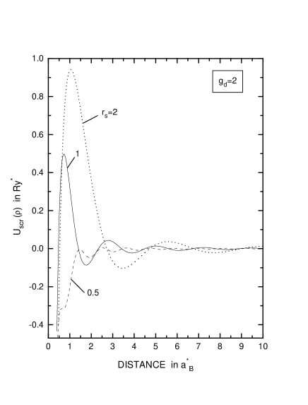
FIG. 2.: Potential energy distribution due to a screened, singly-ionized attractive impurity versus distance. A normal-state, single-valley EL is considered ($g_{d}=2$) at several densities.

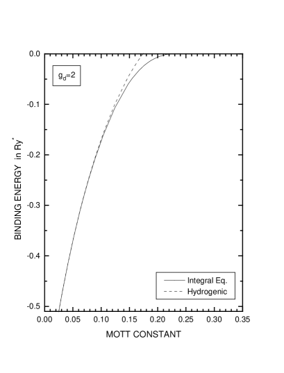
FIG. 3.: Binding energy of a bound impurity electron within a normal-state, single-valley ($g_{d}=2$) 3D EL versus the Mott constant, defined as $a_{B}^{*}n_{3D}^{1/3}$. Solid line refers to integral equation solution which gives a lower energy than the variational treatment based on the hydrogenic wave function denoted by the dashed lines.

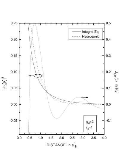
FIG. 4.: Probability distribution of the bound electron wave function within a 2D EL having $r_{s}=1$ and $g_{d}=2$. Solid line is based on the integral equation solution and dashed line refers to 2D hydrogenic wave function, i.e., Eq. (2). Also shown by dotted lines is the screened potential energy experienced by the bound electron.

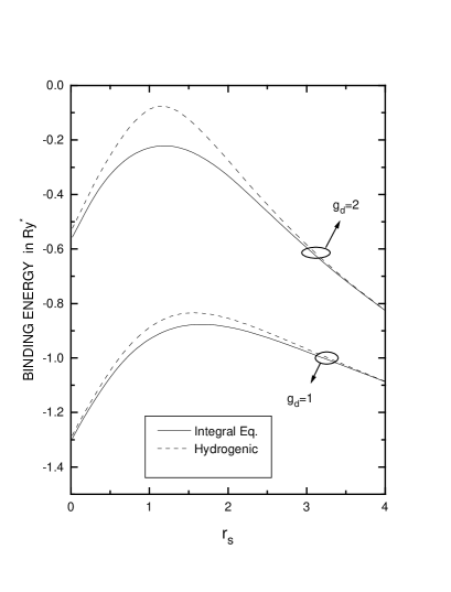
FIG. 5.: Binding energy of a bound electron within a 2D EL versus $r_{s}$ for $g_{d}$=1 and 2. Calculations are based on the integral equation solution (solid lines) and 2D hydrogenic variational wave function (dashed lines).

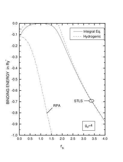
FIG. 6.: Binding energy of a bound electron within a 2D EL versus $r_{s}$ for $g_{d}$=4 (i.e., two valley degeneracy). Solid line denotes the integral equation solution and the dashed line denotes 2D hydrogenic variational wave function result, both utilizing the STLS screening. Dash-dot line refers to RPA screening based on the integral equation solution.

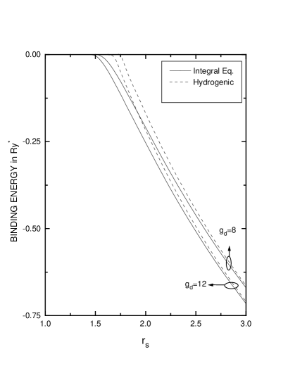
FIG. 7.: Binding energy of a bound electron within a 2D EL versus $r_{s}$ for $g_{d}$=8 and 12 (i.e., four and six valley degeneracies). Solid lines denote the integral equation solutions and the dashed lines denote 2D hydrogenic variational wave function results.

FIG. 8.: Binding energies in 2D EL versus $r_{s}$ based on the integral equation solutions. For comparison purposes several $g_{d}$ values are included.

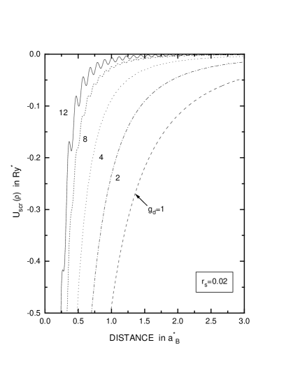
FIG. 9.: Potential energy distribution due to a screened, singly-ionized attractive impurity versus distance. The effect of the degeneracy factor $g_{d}$ is illustrated from spin-polarized ($g_{d}=1$) to six valley degeneracy ($g_{d}=12$); all at a very high density ($r_{s}=0.02$) of a 2D EL.

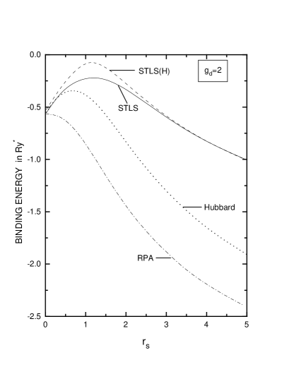
FIG. 10.: The effect of dielectric function on the binding energy for 2D EL using RPA, Hubbard and STLS screenings; all computed by solving the integral equation. Also the STLS screened binding energy is shown based the 2D hydrogenic variational wave function labeled by STLS(H).