Moving glass theory of driven lattices with disorder

Abstract

We study periodic structures, such as vortex lattices, moving in a random pinning potential under the action of an external driving force. As predicted in [T. Giamarchi, P. Le Doussal Phys. Rev. Lett. 76 3408 (1996)] the periodicity in the direction transverse to motion leads to to a new class of driven systems: the Moving Glasses. We analyse using several renormalization group techniques the physical properties of such systems both at zero and non zero temperature. The Moving glass has the following generic properties (in $d\leq 3$ for uncorrelated disorder) (i) decay of translational long range order (ii) particles flow along static channels (iii) the channel pattern is highly correlated along the direction transverse to motion through elastic compression modes (iv) there are barriers to transverse motion. We demonstrate the existence of the “transverse critical force” at $T=0$ and study the transverse depinning. A “static random force” both in longitudinal and transverse directions is shown to be generated by motion. Displacements are found to grow logarithmically at large scale in $d=3$ and as a power law in $d=2$. The persistence of quasi long range translational order in $d=3$ at weak disorder, or large velocity leads to the prediction of the topologically ordered “Moving Bragg Glass”. This dynamical phase which is a continuation of the static Bragg glass studied previously, is shown to be stable to a non zero temperature. At finite but low temperature, the channels broaden but survive and strong non linear effects still exist in the transverse response, though the asymptotic behavior is found to be linear. In $d=2$, or in $d=3$ at intermediate disorder, another moving glass state exist, which retains smectic order in the transverse direction: the Moving Transverse Glass. It is described by the Moving glass equation introduced in our previous work. The existence of channels allows to naturally describe the transition towards plastic flow. We propose a phase diagram in temperature, force and disorder for the static and moving structures. For correlated disorder we predict a “moving Bose glass” state with anisotropic transverse Meissner effect, localization and transverse pinning. We discuss the effect of additional linear and non linear terms generated at large scale in the equation of motion. Generalizations of the Moving glass equation to a larger class of non potential glassy systems described by zero temperature and non zero temperature disordered fixed points (dissipative glasses) are proposed. We discuss experimental consequences for several systems, such as anomalous Hall effect in the Wigner crystal, transverse critical current in the vortex lattice, and solid friction.

I Introduction

Interacting systems which tend to form spontaneously periodic structures can exhibit a remarkable variety of complex phenomena when they are driven by an external force over a disordered substrate. Many of these phenomena, which arise from the interplay between elasticity, periodicity, quenched disorder, non linearities and driving, are still poorly understood or even unexplored. For numerous such experimental systems, transport experiments are usually a convenient way to probe the physics (and sometimes the only way when more direct methods - e.g. imaging are not available). It is thus an important and challenging problem to obtain a quantitative description of their driven dynamics. Vortex lattices in type II superconductors are a prominent example of such systems [3]. The motion of the lattice under the action of the Lorentz force (associated to a transport supercurrent) in the presence of pinning impurities has been studied in many recent experiments [4, 5, 6, 7, 8, 9, 10] There are other examples of well studied driven systems where quenched disorder is known to be important, such as the two dimensional electron gas in a magnetic field which forms a Wigner crystal [11, 12, 13] moving under an applied voltage, lattices of magnetic bubbles [14, 15] moving under an applied magnetic field gradient, Charge Density Waves (CDW) [16] or colloids [17] submitted to an electric field, driven josephson junction arrays [18, 19] etc.. This problem may also be important in understanding tribology and solid friction phenomena [20], surface growth of crystals with quenched bulk or substrate disorder [21], domain walls in incommensurate solids [22]. One striking property exhibited by all these systems is pinning, i.e the fact that at low temperature there is no macroscopic motion unless the applied force $f$ is larger than a threshold critical force $f_{c}$. Dynamic properties have thus been studied for some time, quite extensively near the depinning threshold [23, 24, 25], but mostly in the context of CDW [26, 27, 28] or for models based on driven manifolds [29, 30] and their relation to growth processes [31] described by the Kardar Parisi Zhang (KPZ) equation[32, 29] They are however, far from being fully understood. In addition, the full problem of a periodic lattice (with additional periodicity transverse to the direction of motion) was not scrutinized until very recently [33].

A crucial question in both the dynamics and the statics is whether topological defects in the periodic structure are generated by disorder, temperature and the driving force or their combined effect. Another important issue is to characterize the degree of order (e.g translational order, or temporal order) in the structure in presence of quenched disorder. In the absence of topological defects it is sufficient in the statics to consider only elastic deformations. In the dynamics this leads to elastic flow. On the other hand, if these defects exist (e.g unbound dislocation loops) the internal periodicity of the structure is lost and one must consider also plastic deformations. In the dynamics the flow will then not be elastic but turn into plastic flow with a radically different behaviour.

The statics of lattices with impurity disorder has been much investigated recently, especially in the context of type II superconductors. It was generally agreed that disorder leads to a glass phase (often called [34] a vortex glass) with many metastable states, diverging barriers between these states [35, 3], pinning and loss of translational order. Indeed, general arguments [36, 37], unchallenged until recently, tended to show that disorder would always favor the presence of dislocations destroying the Abrikosov lattice beyond some length scale. In a series of recent works [38, 39, 40, 41], we have obtained a different picture of the statics of disordered lattices (including vortex lattices) and predicted the existence of a new thermodynamic phase, the Bragg glass. The Bragg glass has the following properties: (i) it is topologically ordered (ii) relative displacements grow only logarithmically at large scale (iii) translational order decays at most algebraically and there are divergent Bragg peaks in the structure function in $d=3$ (i.e quasi long range order survives). (iv) it is nevertheless a true static glass phase with diverging barriers. There has been several analytical [42, 43, 44] and numerical studies [45, 46] confirming this theory. The predicted consequences for the phase diagram of superconductors compare well with the most recent experiments [41]

While some progress towards a consistent theoretical treatment has been made in the statics, it is still further removed in the dynamics. Determining the various phases of driven system is still a widely open question. Evidence based mostly on experiments, numerical simulations and qualitative arguments indicates that quite generally one expects plastic motion for either strong disorder situations, high temperature, or near the depinning threshold in low dimensions (for CDW see e.g.[47]). Indeed there has been a large number of studies on plastic (defective) flow [48, 49, 50]. In the context of superconductors a $H$-$T$ phase diagram with regions of elastic flow and regions of plastic flow was observed[51, 9]. Several experimental effects have been attributed to plastic flow, such as the peak effect [52, 9, 53, 54], unusual broadband noise [55] and fingerprint phenomena in the I-V curve [56, 57, 10]. Steps in the $I-V$ curve were also observed in YBCO near melting in [7]. Close to the threshold and in strong disorder situations the depinning is observed to proceed through what can be called “plastic channels” [58, 59] between pinned regions. This type of filamentary flow has been found in [60] in simulations of 2D (strong disorder) thin film geometry (with $c_{11}\gg c_{66}$). Depinning then proceeds via filamentary channels which become increasingly denser. Filamentary flow was proposed as an explanation for the observed sharp dynamical transition observed in MoGe films [57, 10] characterized by abrupt steps in the differential resistance. Also, interesting effects of synchronization of the flow in different channels were observed in [60]. Despite the number of experimental and numerical data [49, 50] a detailed theoretical understanding of plastic motion remains quite a challenge [61].

As in the statics, one is in a better position to describe the elastic flow regime, which is still a difficult problem. This is the situation on which we will focus in this paper. Though elastic flow in some cases extends to all velocities, a natural idea was to start from the large velocity region and carry perturbation theory in $1/v$. At large velocity one may think at first that since the sliding system averages enough over disorder one recovers a simple behavior, in fact much simpler than in the statics. Indeed it was observed experimentally, some time ago in neutron diffraction experiments [62], and in more details recently [63], that at large velocity the vortex lattice is more translationally ordered than at low velocity. This tendency to dynamical reordering has also been seen in numerical simulations [48, 49, 64]. The $1/v$ expansion has been fruitful to compute the corrections to the velocity itself in [65, 66, 27]. Recently it was extended by Koshelev and Vinokur in [67] to compute the vortex displacements $u$ induced by disorder and leads to a description in term of an additional effective shaking temperature induced by motion. This description suggests bounded displacements in the solid and thus a perfect moving crystal at large velocity.

Recently we have investigated [68] the effects of the periodicity of the moving lattice in the direction transverse to motion, in the same spirit which led to the prediction of the Bragg glass in the statics. It was still an open problem how much of the glassy properties remain once the lattice is set in motion. We found that, contrarily to the naive expectation, some modes of the disorder are not affected by the motion even at large velocity. Thus, the large $v$ expansion of [67] breaks down and the effects of non linear static disorder persists at all velocities, leading to new physics. As a result the moving lattice is not a perfect crystal but a moving glass.

The aim of this paper is to provide a detailed description of the moving glass state predicted in [68] and to present our approach to the general problem of moving lattices. A brief account of some of the new results contained here (e.g the $T=0$ renormalization group equations RG and fixed points) has already appeared in [69, 70]. We will use several RG approach at zero and at non zero temperature. Since several Sections of this paper are rather technical we have chosen to expose all the results about the physics of the moving glass in Sections II and III in a self contained manner, avoiding all technicalities. The reader can find there the results for the existence of channels (III A) the transverse I-V curves at $T=0$ and the dynamical Larkin length ( III B ), the random force and the correlation functions ( III C ) the various crossover lengths and the the finite temperature results (III E). Decoupling scenarios which distinguish between the Moving Bragg glass and the Moving transverse glass ( III D) as well as predictions for the dynamical phase diagrams are also given in ( III F) Finally we discuss how the moving glass theory stands presently compared to numerical simulations ( III G) and experiments (III H) and present some suggestions of further observables which would be interesting to measure.

The following Sections are devoted to making progress in an an analytic description of the moving state of interacting particles in a random potential. Since this is a vastly difficult problem, it is potentially dangerous (and unfruitful) to try to attack this problem by treating all the effects at the same time (dislocations, non linearities, thermal effects etc..). Already within the simplifying assumption of an elastic flow two main types of phenomena are missed in a naive large $v$ approach. The first one is a direct consequence of previous works on driven dynamics of CDW and elastic manifolds [32, 29]. It is expected on symmetry grounds [71] that new non linear KPZ terms $(\nabla u)^{2}$ will be generated by motion, an effect which was studied in the driven liquid [72]. Another important effect, studied so far only within the physics of CDW, is the generation of a static random force convincingly argued by Krug [73] and explored in [74]. If both effects are assumed to occur simultaneously, they may lead to interesting interplays which have been explored only recently and only in simple CDW models [75]. However there still no explicit RG derivation of those terms even in CDW models. In the context of driven lattices, there are not even discussed yet. Our aim in this paper is to remedy this situation. We derive these terms explicitly and show that other linear terms, a priori even more relevant are generated. Though these additional linear, non linear and random force terms certainly complicate seriously the problem, focusing exclusively on these terms only obscurs the physics of the present problem. Indeed the second and as we show here more important effect in the moving structure is the crucial role of transverse periodicity to describe the dynamics.

A rigorous study of the problem of moving interacting particules would be to first study the fully elastic flow of a lattice. Once the main elastic physics is understood a second step is then to allow for topological excitations (vacancies, interstitials, dislocations). In principle the results obtained within the elastic only approach can, as in the statics, be used to check self consistently the stability of the elastic flow itself. It is hard to see how one can do that in a controlled way without some detailed understanding the elastic flow first ! Here we carry most of the first step and propose an effective description of the second.

Even the purely elastic model turns out to be difficult to treat when all sources of anisotropies, non linear elasticity, cutoff effects are included. There are no analogous terms in the statics and thus in that sense the dynamics is more difficult. Our strategy has thus been to simplify the problem in several stages and resort to simplified models. The simplified models of Moving glasses that we have obtained turn out to exhibit some new physics and become interesting in their own. They call for interesting generalizations to other models exhibiting dissipative glassy behaviour, as we will propose.

We will call Model I the full model of an elastic flow of a lattice containing all the above mentionned relevant linear and non linear terms. Such models can also be written for other elastic structures with related kind of order (such as liquid crystal order). This model will be discussed in Section VIII B. However its complete study goes beyond the present paper.

Fortunately, a useful and further simplified model can be constructed (Model II). It corresponds to considering the above full elastic model in the continuum limit. It will certainly give a very good approximation of the full model at least up to some very large scale. This model was discussed in [68] and is studied in details here. It has both longitudinal degrees of freedom (along the direction of motion) and transverse ones. Though it is quite difficult, it can be handled by perturbative renormalization group studies, as we will show here. It has a new and non trivial fixed point which gives a detailed description of the moving Bragg glass phase.

It turns out that most of the physics of Moving glass is contained in a further simplification of Model II which retains only the transverse degrees of freedom (displacements). This model, which here we call Model III, was introduced in Ref. [68] and is described by the equation of motion:

$$\eta\partial_{t}u+\eta v\partial_{x}u = c\nabla^{2}u+F^{\text{stat}}(r,u(r,t))+\zeta(r,t)$$ (1)

which we call the moving glass equation. $F^{\text{stat}}$ is a non linear static pinning force and we have denoted $x$ the direction of motion, $y$ the transverse direction(s) and $r=(x,y)$. The model retains only the transverse displaceemnt $u\equiv u_{y}$.

Equation (1) was obtained simply by considering the density modes of the moving structure which are uniform in the direction of motion. Indeed, the key point of Ref. [68] is that the transverse physics is to a large extent independent of the details of the behaviour of the structure along the direction of motion. This is because the transverse density modes, which can be termed smectic modes, see an almost static disorder and thus are the most important one to describe the physics of moving structures with a periodicity in the direction transverse to motion! Let us emphasize that this is explicitly confirmed here by the detailed RG analysis of the properties of Model II. Note that to obtain Model III one sets formally $u_{x}=0$ [76].

The hierarchy of models introduced here is represented in Fig. 1.

FIG. 1.: Various models studied here to describe with various levels of approximation the (i) fully elastic flow of a lattice (ii) intermediate phase with ordering transverse to motion (iii) plastic flow

The outline of the paper is as follows. After the Sections II and III where we give a non technical discussion of the physical results, we start in Section IV by deriving an equation of motion and, carefully examining its symmetries, we introduce the Models I,II,III and explain the approximations leading to them. In Section V we perform perturbation theory on the full dynamical problem, focusing on Model II. In Section VI we use the functional RG to study Model III and thus the transverse physics in $d=3$ and $d=3-\epsilon$. We study $T=0$ and $T>0$. In Section VII we study a two dimensional version of the moving glass equation Model III. This allows to obtain results in $d=2$ at $T>0$ and in $d=2+\epsilon$. Having obtained a good understanding of the transverse physics in the previous sections, we attack in Section VIII A the RG of Model II. Finally in Section VIII B we examine the full Model I, show that linear terms and KPZ terms are generated at large scales and discuss some consequences.

II Moving structures and moving glasses

A Moving structures: general considerations

All the structures we consider share the same basic features. The static system in the absence of quenched substrate disorder consists of a network of interacting objects at equilibrium positions $R_{i}^{0}$, forming either a perfect lattice (periodic case) or elastic manifolds (non periodic case). Depending on the system the objects can be either pointlike (e.g. electrons in a Wigner crystal) or lines (vortex lines in superconductors ). Deformations away from equilibrium positions are described by displacements $u_{i}$ or in a coarse grained description $u(r,t)$ where $r$ is the internal coordinate. A complete characterization of the structure in motion uses three parameters (i) the internal dimension $D$ (ii) the number of components $n$ of the displacement field $u_{\alpha}$ and (iii) the embedding space dimension $d$. Two examples are shown in Figure 2 and more details are given in the Appendix. Since we are mostly interested here in periodic structures (though not exclusively) we can set $D=d$. We will consider motion along one direction called $x$, and we parametrize throughout all this paper the space variable $r$ as $r=(x,y,z)$ where $x$ is one dimension, $y$ has a priori $n-1$ dimensions and $z$ has $d_{z}=d-n$ dimensions, and the displacements along motion as $u_{x}$ and transverse to motion as $u_{y}$. Three dimensional triangular flux lines lattices driven along a lattice direction thus have $d=3,n=2$, $r=(x,y,z)$, $u=(u_{x},u_{y})$ where $z$ denotes the direction of the magnetic fields. Two dimensional triangular lattices of point vortices have $d=2,n=2$, $r=(x,y)$.

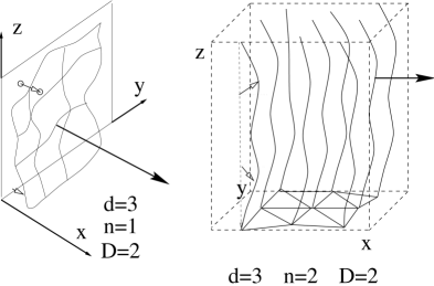
FIG. 2.: Two cases of a driven structure. An interface $D=2$, $n=1$, $d=3$, driven orthogonal to its internal space. A triangular line lattice $D=3$, $n=2$, $d=3$ driven within its internal space

At finite temperatures or in the presence of quenched substrate disorder the structure is deformed. An important issue is then to characterize the degree of order. This can be expressed in terms of displacements correlation functions. The simplest one measures the relative displacements of two points (e.g two vortices) separated by a distance $r$.

$$\tilde{B}(r)=\frac{1}{n}\overline{\langle[u(r)-u(0)]^{2}\rangle}$$ (2)

where $\langle\rangle$ denotes an average over thermal fluctuations and $\overline{\qquad}$ is an average over disorder. The growth of $\tilde{B}(r)$ with distance is a measure of how fast the lattice is distorted. For thermal fluctuations alone in $d>2$, $\tilde{B}(r)$ saturates at finite values, indicating that the lattice is preserved. Intuitively it is obvious that in the presence of disorder $\tilde{B}(r)$, will grow faster and can become unbounded. $\tilde{B}(r)$ can directly be extracted from direct imaging of the lattice, such as performed in decoration experiments of flux lattices.

Related to $\tilde{B}(r)$ is the structure factor of the lattice, obtained by computing the Fourier transform of the density of objects $\rho(r)=\sum_{i}\delta^{d}(r-R^{0}_{i}-u_{i})$. The square of the modulus $|\rho_{k}|^{2}$ of the Fourier transform of the density is measured directly in diffraction (Neutrons, X-rays) experiments. For a perfect lattice the diffraction pattern consists of $\delta$-function Bragg peaks at the reciprocal vectors. The shape and width of any single peak around $K$ can be Fourier transformed to obtain the translational order correlation function given by

$$C_{K}(r)=\overline{\langle e^{iK.u(r)}e^{-iK.u(0)}\rangle}$$ (3)

$C_{K}(x)$ is therefore a direct measure of the degree of translational order that remains in the system. Three possible cases are shown in figure 3.

FIG. 3.: Various possible decays of $C_{K}(r)$. (a) For thermal fluctuations alone $C_{K}(r)\to{\rm Cste}$, one keeps perfect $\delta$ function Bragg peaks, albeit with a reduced weight (the Debye-Waller factor). (b) $C_{K}(r)$ decays exponentially fast. The structure factor has no divergent peak any more, so translational order is destroyed beyond length $R_{a}$, although some degree of order persists at short distance. (c) $C_{K}(r)$ decays as a power law. The structure factor still has divergent peaks but not sharp $\delta$ function ones. One retains quasi-long range translational order. This is for example the case in $d=2$ at small temperature (Kosterlitz-Thouless) or in the Bragg glass.

For simple Gaussian fluctuations (and isotropic displacements) $C_{K}(r)=e^{-\frac{K^{2}}{2}\tilde{B}(r)}$ but such a relation holds only qualitatively in general (as a lower bound). Depending on how much cristalline order remains in the system the structure factor will have extremely different behaviors as depicted in figure 4.

FIG. 4.: Depending on the translational order remaining in the lattice the structure factor has different shapes. The thick line is the $\delta$ function Bragg peak of a perfect lattice (including thermal fluctuations). The dashed line is the power-law Bragg peak of the Bragg glass (which retains quasi long range order and has no topological defects), the dotted line is the lorentzian-like shape of a system loosing its translational order exponentially fast.

Quite surprisingly, if one takes into account correctly the periodicity of the lattice, a thermodynamic phase without dislocations was predicted to exist in $d=3$ at weak disorder. [38, 39]. This phase, named the Bragg Glass, posses quasi long range order with Bragg peaks diverging as least as $q^{-(3-A_{3})}$ (with $A_{3}\approx 1$), similar to dashed line in Fig. 4 At the same time displacements $B(r)$ grow logarithmically at large scale [38, 39]. Similar predictions hold for other elastic models such as random field XY systems, and a priori also for liquid crystals. The Bragg glass theory has by now received considerable numerical [45, 46] and analytical confirmations [42, 43, 44].

If disorder is increased above a threshold it is predicted that there is a transition at which topological defects proliferate. They destroy the translational long range order exponentially fast beyond a length $R_{D}$ leading to finite height diffractions peaks. The height of the peak will be inversely proportional to the scale at which translational order is destroyed. This transition is thus characterized by the loss of the divergence in the Bragg peaks. In type II superconductors it implies that there is a transition, upon increasing the magnetic field [39], from the Bragg glass (at low fields) to another phase. The high field phase is either the putative vortex glass [34, 36] or is simply continuously related to the high temperature phase. These predictions for the phase diagrams of superconductors has received experimental support (see Ref. [41] for a review).

What happens when an external force is applied to such a structure ? One obviously important quantity to determine is the curve of velocity $v$ versus the applied force $f$. Through this $v-f$ characterics, three main regimes can be distinguished and are shown on Figure 5.

FIG. 5.: A typical $v-f$ characteristics at $T=0$ (full line) and finite temperatures (dashed line). Three main regimes can be distinguished: the creep regime for forces well below threshold, the critical regime around the threshold and the large velocity regime well above threshold.

Far below the depinning threshold $f_{c}$ the system moves through thermal activation. This is the so called creep regime. Since the motion is extremely slow in this regime, it has been analyzed based on the properties of the static system [35, 3]. The resulting $v-f$ curve crucially depends on whether the static system is in a glass state (such as the Bragg Glass) where the barriers $U(f)$ become very large when $f\to 0$, or a liquid where barriers remain finite at small $f$, resulting in a linear resistivity. The general form expected in the creep regime is:

$$v\sim\rho_{0}fe^{-U(f)/T}$$ (4)

Let us emphasize that this “longitudinal” $v-f$ characteristics has mainly be used to determine whether the the static system (i.e the limit $f=v=0$) is or not in a glass state. It may not be enough though, if one wants to probe glassiness of the moving system itself.

The second regime, near the depinning transition $f\approx f_{c}$, has been intensely investigated in similarity with usual critical phenomena (see e.g [23, 24, 25]) where the velocity plays the role of an order parameter. A particularly important question is that regime is to determine whether plastic rather than elastic motion occurs. Close to the threshold in low dimensions and in strong disorder situations the depinning is observed to proceed through “plastic channels” [58, 59] between pinned regions. This type of filamentary flow has been found in [60] in simulations of 2D (strong disorder) thin film geometry (with $c_{11}\gg c_{66}$) where depinning proceeds via filamentary channels which become increasingly denser.

FIG. 6.: Plastic flow of a network of objects submitted to an external force $F$, shown for simplicity in two dimensions. The motion occurs through plastic channels around pinned regions. Plastic flow might occur close to the depining threshold whereas at large velocities one expects to recover elastic flow where the whole lattice moves coherently.

The third regime is above the depinning threshold $f>f_{c}$ This is situation on which we will focus in this paper (though some of our considerations will have consequences in the other regimes as well). An important phenomenon in this regime is that of dynamical reordering. Indeed, it was observed experimentally, some time ago in neutron diffraction experiments [62], and in more details recently [63], that at large velocity the vortex lattice is more translationally ordered than at low velocity. Intuitively the idea is that at large velocity $v$, the pinning force on each vortex varies rapidly and disorder should produce little effect. This phenomenon was also known in the context of CDW [23]. The tendency to reorder has also been seen in numerical simulations [48, 49, 64].

Since the effect of disorder were expected to vanish at high velocity perturbation theory in $1/v$ were developped mainly to compute the $v-f$ characteristics [65, 66, 27]. Recently it was extended by Koshelev and Vinokur in [67] to compute the vortex displacements $u$ induced by disorder in the moving lattice and in the moving liquid. The effect of disorder on the moving liquid was found to be equivalent to heating to an effective temperature $T^{\prime}=T+T_{sh}$ with $T_{sh}\sim 1/v$. Thus the moving liquid was argued to survive at temperatures lower than the melting temperature $T<T_{m}$, and a dynamical melting transition to occur below $T_{m}$ from a moving liquid to a moving solid upon increase of the velocity [67], when $T^{\prime}=T_{m}$. These arguments were then extended to describe the moving solid itself, and it was argued that there the effect of pinning could also be described [67] by some effective shaking temperature $T_{sh}\sim 1/v^{2}$ defined by the relation $<|u(q)|^{2}>=T_{sh}/c_{66}q^{2}$. This suggests bounded displacements in the solid and that at low $T$ and above a certain velocity the moving lattice is a perfect crystal. As will be discussed in the remainder of this paper the picture of the moving lattices emerging from the above bold qualitative arguments [67] goes wrong in several ways.

There are several other important questions to be answered in addition to the $v-f$ characteristics. The first one is the question of the effect of the motion on the spatial correlations and in particular whether translational order exist in a moving system. This is related to the question of plastic versus elastic flow. If plastic flow occurs, the structure factor should signal some destruction of lattice. However because a moving system is inherently anisotropic new effects may appear and the decay of the structure factor will not be as isotropic as in the static system (the Lorentzian in Figure 4). This question thus remains to be investigated. A possibility, suggested by the idea of a shaking temperature [67], would be that at large velocity one should observe $\delta$-function Bragg peaks characteristic of a crystal a finite temperature. Such questions will be discussed in details in section III. Finally determining how motion affects the phase diagram of the statics has to be investigated and depends of course on the above issues. In particular what remains of the glassy properties of the systems when in motion (slow relaxation, history dependence, non-linear behaviors) needs to be addressed.

For moving periodic systems, an equivalent question can be asked also about “temporal order” and its associated effects such as noise spectrum. In particular if one looks at a signal at a fixed position in space but as a function of time, one expects a periodic signal with a periodicity of $a/v$, having $\delta$ peaks in frequency at the multiples of the washboard frequency $\omega_{0}=2\pi v/a$. If the lattice becomes imperfect one could naively expect the Fourier peaks in frequency to broaden in a way that reflects the loss of translational order. Quite surprisingly this is not so. Indeed it can be shown for a single component displacements field (CDW) [77] that the perfect periodicity in time remains (in the absence of topological defects). However this result is not readily applicable to a moving lattice, and it is thus crucial to determine whether this remarkable property holds in that case.

B The Moving Glass

To tackle the physics of a structure with a displacement field with more than one component ($n>1$), such as a triangular lattice (by contrast with a single $Q$ CDW), two routes seem to be possible. The commonly followed one [74, 67, 78] is to simply borrow from, or extend, the physics of single component CDW [26, 27, 28], or of elastic manifolds driven perpendicularly to their internal direction [29]. In this case emphasis is put on the displacements along the direction of motion $u_{x}$ and on the proper way to model its dynamics. Such a problem has turned out to be already quite complicated in particular due to the generation of KPZ type non linearities in the equation of motion. Even if degrees of freedom transverse to motion $u_{y}$ exist as in the cases depicted in Figure 7 they constitute an extension [30] of this “longitudinal” physics. Thus in this “CDW paradigm” it would seem necessary to understand first completely the physics of longitudinal modes $u_{x}$ and then incorporate $u_{y}$ as an extra complication. Indeed there were a few attempts to describes the physics of driven vortex lattices along those lines [67, 74].

FIG. 7.: Three types of dynamical systems. (a) a manifold driven perpendicular to itself. (b) a single Q CDW system. Only displacements in the directions of motion exist, but periodicity along the direction of motion can play a role. (c) A periodic system with transverse degrees of freedom driven along one of its symmetry directions. The correct description of this last class of systems is the moving glass fixed point where the transverse degrees of freedom are the important one as represented here.

The second approach is based on the realization that the physics of periodic structures driven along one of their internal direction is radically different [68] from the above descriptions. This stems from the fact that due to the periodicity in the transverse direction $u_{y}$ a static non linear pinning force $F^{\rm{stat}}$ persists even in a fast moving system. We want to stress that this is a very general property of a any moving structure which contains uniform density modes $K_{x}=0$ in the direction of motion (as can be seen on the Fourier decomposition of the density [68]). As illustrated in Fig. 7 the substructure formed by these modes can deform elastically in the $u_{y}$ direction and sees essentially a static disorder. As is obvious from the picture 7 (c), this substructure has generically a liquid crystal type of (topological) order and can be termed a “smectic” (though when $d_{z}=0$, e.g for $d=3$ and $n=3$, it is rather a “line crystal” - see below). In all cases the basic starting point thus involves the transverse degrees of freedom as shown on figure 7, and is quite different from the “CDW description”. The equation which capture the main ingredients of such moving systems was derived in Ref. [68]. It leads to a new and interesting model for transverse components $u\equiv u_{y}$, which has the general form in the laboratory frame:

$$\eta\partial_{t}u+\eta v\partial_{x}u = c\nabla^{2}u+F^{\text{stat}}(r,u(r,t))+\zeta(r,t)$$ (5)

Since this equation captures glassy features of moving systems we call it the moving glass equation. Although it looks like a standard pinning equation the convection term $\eta v\partial_{x}u$ dissipates even in the static limit (a reminder that we are looking at a moving system) and does not derive from a potential. Thus we will consider this problem and its generalizations as a prototype for a new class of physical phenomena which are glassy and do not derive from a potential (or from a hamiltonian). The first example is to choose $F^{\text{stat}}(r,u)$ periodic in the $u$ direction:

$$F^{\text{stat}}(r,u_{y}) = V(r)\rho_{0}\sum_{Ky\neq 0}K_{y}\sin{K_{y}(u_{y}-y)}$$ (6)

and corresponds to lattices (or to liquid crystals) driven in a random potential with a short range correlator $\overline{V(r)V(r^{\prime})}=g(r-r^{\prime})$ of range $r_{f}$. The study of this case in Ref. [68] gave the first hint that non potential dynamics can indeed exhibit glassy properties and lead to dissipative glasses. This is a rather delicate notion because the the constant dissipation rate in the system would naturally tend to generate or increase the effective temperature and kill the glassy properties. However this type of competition between glassy behaviour and dissipation arises in other systems which are a generalization of the above equation. Let us briefly indicate some of the generalizations that we are proposing which are being studied here or in related works.

An interesting generalization is the case of a periodic manifold with correlated disorder [79]. This is relevant to describe the moving Bose glass state of driven vortex lattices in the presence of correlated disorder.

Another generalization is to extend the equation (5) to a $N$ component vector $u_{\alpha}$. It is easy to see in that case that a non potential non linear disorder is generated if $v>0$ (which reduces to the “static random force” for $N=1$). Thus in that model it is natural to look at a generic non potential disorder $F_{\alpha}^{\text{stat}}(r,u)$ from the start. The mean field dynamical equations for large $N$ and the FRG equations at any $N$ for a large class of such models are derived in Section VI and in Appendix F. A subclass of these models is non periodic models (manifold). They are relevant to describe the random manifold crossover regime in the moving glass (see below). A further subclass is then obtained by setting $v=0$. Interestingly the resulting model describes polymers (and manifolds) in random flows and can be studied both in the large $N$ limit [80] and using RG [81] for any $N$.

Finally, there are other simpler but interesting situations such as disorder correlated along the direction of motion or lattices moving in a periodic tin roof potential. These potentials which are independent of $x$ have the interesting property that the steady state measure $P[u(r)]$ is identical (at any $T>0$) to the one with $v=0$.

Thus we see that the moving glass equation hides a whole class of new interesting dissipative models whith glassy properties.

III Physical results

In this Section we present all the physical results on the Moving Glass that we have obtained in Ref. [68, 69, 33] and in the present paper. We deliberately avoid technicalities and refer to the proper Sections for details.

A Channels

One of the most striking property of moving structures described by (5) is that the non linear static force $F^{\rm{stat}}$ results in the pinning of the transverse displacements $u_{y}(r,t)$ into preferred static configurations $u_{y}(r)$ in the laboratory frame. Thus the resulting flow can be described in terms of static channels where the particles follow each others like beads on a string. In the laboratory frame these channels are determined by the static disorder and do not fluctuate in time. They can be visualized in simulations or experiments by simply superposing images at different times. What makes the problem radically new compared to conventional systems which exhibit pinning is that despite the static nature of these channels there is constant dissipation in the steady state. This can be seen in the moving frame where each particle, being tied to a given channel (which is then moving) must wiggle along $y$ and dissipate. In fact the existence of the channels shows in a transparent way that the wiggling of different particles in the moving frame is highly correlated in space and time, thus leading to a radically different image as the one embodied in the “shaking temperature” based on thermal like incoherent motion [67].

The channels are thus the easiest paths followed by the particles. One can see that the “cost” of deforming a channel along $y$ is that dissipation is increased. Thus the channels are determined by a subtle and novel competition between elastic energy, disorder and dissipation. As a consequence these channels are rough. This is a crucial difference between what would be observed for a perfect lattice as illustrated in Figure 8

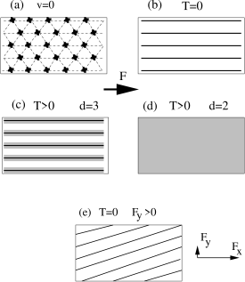
FIG. 8.: (a) a snapshot of a perfect (non-disordered) lattice moving along the $x$ direction. (b) upon superposing images at different times one would see that at $T=0$ the particles follow perfectly straight lines. (c) at $0<T<T_{m}$ in $d=3$ the channels remain perfectly straight with a finite width due to the thermal fluctuation of the particles. (d) in $d=2$ since thermal fluctuations are unbounded channels are completely blurred and cannot be defined even for $T<T_{m}$. (e) Even in situation (b), (c) applying a additional small force along $y$ immediately results in tilted channels with angle $F_{y}/F_{x}$.

By contrast the channels which are predicted in the Moving Glass are illustrated in Figure 9 and in Figure 10. It is important to stress that the Moving Glass equation (5) introduced in [68] does not assume anything about the coupling of the particle in different channels but only implies that the channels themselves are elastically coupled along $y$, and thus through compression modes. Indeed on specific models such as model II one can verify explicitely that although coupling between longitudinal and transverse degrees of freedom exists a priori, the longitudinal degrees of freedom $u_{x}$ do not feed back at all in the moving glass equation (see section VIII A).

The existence of channels naturally leads to several a priori possible regimes for the coupling between particles in different channels. The first case, represented in Fig. 9 (b), is a topologically ordered moving structure corresponding to full elastic coupling between particles in different channels. Since, remarkably, this structure retains perfect topological order despite the roughness of the channels, it is reminiscent of the properties of the static Bragg glass, and thus we call it a Moving Bragg glass. A second case of a Moving Glass corresponds to decoupling between the channels, by injections of dislocations beyond a certain lengthscale $R_{d}$ and is called the Moving Transverse Glass. These two regimes will be discussed in more details in section III D. Finally note that in $d=3$ channels can be either “sheets” (for line lattices) or linear (for point lattices) as represented in Fig. 10.

It is important to note that the channels in the Moving glass are fundamentally different in nature from the one introduced previously [58, 59] to describe slow plastic motion between pinned islands, as illustrated in Fig. (6). In the Moving glass they form a manifold of almost parallel lines (or sheets for vortex lines in $d=3$), elastically coupled along $y$. For that reason we call them generically “elastic channels” (whether or not they are fully coupled or decoupled) to distinguish them from the “plastic channels” (even though some plastic flow may occur when elastic channels decouple).

Note that in the above discussion we have concentrated on elastic channels which can spatially decouple. It is possible a priori that they may still remain temporally coupled, i.e synchronized. Indeed, examples of synchronization where observed even in extremely plastic filamentary flow.

FIG. 9.: (a) The motion in the moving glass occurs through rough static channels. Relative deformations grow with distance and become of order $a$ at distances $R_{a}^{x}\sim{R_{a}^{y}}^{2}$. Only the channels themselves are elastically coupled along the $y$ direction. Depending on the dimension, velocity and disorder strength two main cases can occur: (b) an elastic flow where the particles positions are elastically coupled between channels (in $d=3$ and weak disorder or large velocities). In this regime the lattice is topologically ordered (no dislocations) and the rows of the lattice follow the channels. This is a Moving Bragg Glass. (c) In $d=2$ or at stronger disorder in $d=3$ the positions of particles in different channels may decouple. Dislocations with Burgers vectors along $x$ (indicated by the square) are then injected between some channels beyond the length $R_{a}$. This situation describes a Moving transverse glass (with a smectic or a line crystal type of topological order).

FIG. 10.: Different types of topological order for the manifold of channels in $d=3$ (a) for line lattices in motion the channels are “sheets” and thus form an anisotropic type of smectic layering (b) for 3d lattices of pointlike objects or for triply periodic structures (triple $Q$ CDW) they have instead the topology of a line crystal

B Dynamical Larkin length and transverse critical force

Another important property of the moving glass intimately related to the existence of stable channels is the existence of “transverse barriers”. Indeed it is natural physically that once the pattern of channels is established the system does not respond in the transverse direction along which it is pinned. Thus we have predicted in Ref. [68] that the response to an additional small external force $F_{y}$ in the direction transverse to motion vanishes at $T=0$. A true transverse critical force $F^{y}_{c}$ exists (and thus a transverse critical current $J^{y}_{c}$ in superconductors) for a lattice driven along a principal lattice direction.

The transverse critical force is a rather subtle effect, more so than the usual longitudinal critical force. It does not exist for a single particule at $T=0$ moving in a short range correlated random potential. By contrast even a single particule experiences a non zero longitudinal critical force. It does not exist either for a single driven vortex line or any manifold driven perpendicular to itself in a pointlike disordered environment. It would exist however, even for a single particle if the disorder is sufficiently correlated along the direction of motion (such as a tin roof potential constant along $x$ and periodic along $y$). Such disorders break the rotational symmetry in a drastic way. Still, in the case of a lattice driven in an uncorrelated potential it does seem to break the rotational symmetry of the problem. In some sense in the Moving glass the transverse topological order which persists (and the elasticity of the manifold) provide the necessary correlations (through a spontaneous breaking of rotational symmetry). Thus the transverse critical force is a dynamical effect due to barriers preventing the channels to reorient.

We have investigated the equation 5 numerically in $d=2$ and found that indeed starting from a random configuration and at zero temperature the field $u(r,t)$ relaxes towards a static configuration $u_{stat}(r)$ solution of the static equation. Applying a small force in the $y$ direction (i.e adding $f_{y}$ in 5) yields no response. The manifold is indeed pinned.

Thus we have proposed the Moving Glass as a new dynamical phase (a new RG fixed point) and the transverse critical force as its order parameter at $T=0$. The upper critical dimension of this phase is $d=3$ instead of $d=4$ for the static Bragg glass. Above $d=3$ weak disorder is irrelevant and the moving glass is a moving crystal. For $d\leq 3$ disorder is relevant in the moving crystal and leads to a breakdown of the $1/v$ expansion of [67]. Divergences in perturbation theory can be treated using a renormalization group RG procedure (Section VI). One indeed finds a new fixed point which confirms the prediction that the moving glass is a new dynamical phase. Using RG and the properties of this new fixed point one can compute various physical quantities (Section VI B 3). We find that the transverse critical force is given by:

$$F_{c}^{y}\sim A\frac{c~{}r_{f}}{(R^{y}_{c})^{2}}$$ (7)

with $c=c_{11}$ in $d=2$, $c=\sqrt{c_{11}c_{44}}$ in $d=3$ and $A$ is a nonuniversal constant. The length scale $R_{c}^{y}$ is the dynamical Larkin length. It is defined as the length scale along $y$ at which perturbation theory breaks down, non analyticity appears in the FRG and the (scale dependent) mobility vanishes. Before we proceed further let us define now disorder strength parameters. For uncorrelated disorder the random potential $V(r)$ which couples to the density of the structure has short range correlations of range $r_{f}$, $\overline{V(r,z)V(r^{\prime},z)}=g(r-r^{\prime})\delta^{d_{z}}(z-z^{\prime})$ (see Section IV). As in [68] we denote by $\Delta$ (also denoted $\Delta(u=0)$, see Section IV) the bare static pinning force correlator $\Delta=\rho_{0}^{2}\sum_{K_{y},K_{x}=0}K_{y}^{2}g_{K}$ where $\rho$ is the average density and $g_{K}$ the Fourier transform of $g(r)$ at the reciprocal lattice vectors. Throughout $\Delta_{2}$ will denote the second derivative of the non linear pinning force correlator $\Delta_{2}=-\Delta^{\prime\prime}(0)\approx\Delta/r_{f}^{2}$ (see Section VI). Our result is that in $d=3$ the dynamical Larkin length is given by

$$R_{c}^{y}\sim a\exp{\frac{4\pi\eta vc}{\Delta_{2}}}$$ (8)

while in $d\leq 2$ it reads

$$R_{c}^{y}\sim(1+\frac{4\pi\eta vc(3-d)}{\Delta_{2}})^{1/(3-d)}$$ (9)

with again $c=c_{11}$ in $d=2$ and $c=\sqrt{c_{11}c_{44}}$ in $d=3$. These results are valid for large enough velocities $v\gg v^{*}_{c}$ (see below for the definition of $v^{*}_{c}$ and results for all velocities). Note that for $v>v*_{c}$ the dynamical Larkin length depends only on $c_{11}$ (and of $c_{44}$ in $d=3$) as it should since the physics of the moving glass is controlled by the compression modes and thus largely independent of the detailed behaviour along $x$.

Another way to estimate the Larkin length is to compute the displacements in perturbation theory of the disorder. At very short distance one can treat the pinning force in (5) to lowest order in $u$. This gives a model where disorder is described by a random force $F^{\text{stat}}(x)$ independent of $u$ whose correlator is $\langle F^{\text{stat}}(r)F^{\text{stat}}(r^{\prime})\rangle=\Delta\delta^{d}(r-r^{\prime})$. This regime is the equivalent of the short distance Larkin regime for the statics. In the Moving glass at very large velocity $v\gg v_{c}^{*}$ the displacements along $y$ grow as $B(r)=B_{RF}(r)$ (at $T=0$) with:

$$B_{RF}(y)=\int\frac{dq_{x}dq_{y}d^{d_{z}}q_{z}}{(2\pi)^{d}}\frac{\Delta(1-\cos(q_{y}y))}{(\eta vq_{x})^{2}+(c_{11}^{2}q_{y}^{2}+c_{44}^{2}q_{z}^{2})^{2}}$$ (10)

The scale along $y$ at which $u_{y}$ becomes of order $r_{f}$ defines the dynamical Larkin length $R_{c}^{y}$, i.e $B_{RF}(y=R_{c}^{y},x=0)\sim r_{f}^{2}$. The resulting expression coincides with the one obtained within the RG approach (up to non universal prefactors).

Similarly one can define a Larkin length for transverse pinning along the $x$ direction by the condition that $u_{y}(x=R_{c}^{x},y=0)-u_{y}(x=0,y=0)\sim r_{f}$. Since what determines this length is only $u_{y}$ (and not $u_{x}$) it is independent of the detailed behaviour along $x$. It is important to note that the Moving glass is a very anisotropic object at large scale with a scaling $x\sim y^{2}$ of the internal coordinates. This implies that at large velocity ($v>v_{c}^{*}$) the Larkin length along $x$ is very large (much larger than $R_{c}^{y}$), with $R_{x}=v(R_{c}^{y})^{2}/c_{11}$ (One has also the more conventional behaviour $R_{c}^{z}\sim\sqrt{c_{44}/c_{11}}R_{c}^{y}$ in $d=3$ ). Estimating the random force acting on a Larkin volume for the transverse displacements [68] one recovers the above estimate for $F_{c}^{y}$.

The resulting transverse I-V characteristics at $T=0$ is depicted in Fig. 11. The transverse depinning is studied in Section VI and we find the behaviour near the threshold $v_{y}\sim|F^{y}-F_{c}^{y}|^{\theta}$ for $F^{y}>F_{c}^{y}$ with $\theta=1$ to lowest order in $\epsilon$. A reasonable conjecture which would be interesting to verify is that it remains $\theta=1$ to all orders. Thus it starts linearly with a slope which depends on the velocity $v$. It is very large for $v\ll v_{c}^{*}$ and diverges in the limit $v\to 0$.

FIG. 11.: Transverse $v$-$f$ characteristics at $T=0$: transverse velocity $v_{y}$ as a function of the applied transverse force $F_{y}$ at a fixed longitudinal velocity. The behaviour near threshold is found to be linear with a large slope for $v\leq v^{*}_{c}$.

The existence of a transverse critical force in a moving state raises interesting issues about history dependence. These issues are largely open and should be explored in further numerical, experimental and theoretical work.

Let us for instance consider consider two experiments. In the first one a force $f_{x}e_{x}+f_{y}e_{y}$ is applied to the lattice at time $t=0$ and then wait until a steady state is reached. The velocity is then $(v_{x}(f),v_{y}(f)$. In the second experiment one first apply a force $f_{x}$ along the direction $x$, wait for a steady state and then apply $f_{y}$ along $y$. One then measures the velocities $(v^{w}_{x}(f),v^{w}_{y}(f)$. The question is should one find the same result in the two experiments or not. Of course there are subtle issues which complicate the problem and needs to be further investigated (such as (i) the order of the limit system size versus waiting time before deciding a steady state is reached (ii) whether the lattice will globally rotate or break into crystallites, (iii) some non universality of $T=0$ dynamics) but one should still be able to find an operational answer. If it is found that there are such history dependence effects then that would be a strong characteristic of a glassy state (it should not happen in the liquid where one expects both answers to be the same, but in the same trivial sense as for a single particle). On the other hand, if no clear history dependence is found it has interesting consequences. We assume in the following that the global orientation of the lattice is unchanged. Then the first consequence is that there is a well defined history-independent global $v$-$f$ function. This function however is non analytic in a large region of the $f_{x},f_{y}$ plane. $v_{y}(f_{x},f_{y})$ should remain zero at least in the region $f_{y}<F_{c}^{y}(v_{x}(f_{x},f_{y}))$ and similar regions near each of the principal symmetry axis of the crystal. This is clearly the result of the FRG calculation presented here. But then one may also guess that it may be non analytic too along other lattice directions (though it is possible that some of the higher symmetry directions be screened by lower ones). The transverse mobility as a function of the angle and the force should exhibit a complex (and rather strange) behaviour which would be interesting to investigate further. A second interesting consequence would be that if in the above described first experiment one chooses a $f_{y}>0$ smaller than $F_{c}^{y}(v_{x})$, the lattice would first glide in the direction of the applied force (as small time perturbation theory would indicate) but would soon change its velocity to lock it along a symmetry axis. It is quite possible that this locking effect exists and be a possible explanation for the behaviour ubiquitously observed in experiments, namely that lattices tend to flow along their principle axis directions. Such a behaviour near depinning was observed in recent decoration experiments [82].

Another important question for experiments is to determine the transverse critical force as a function of the longitudinal velocity $v$. As $v$ decreases $F_{c}^{y}$ increases but it is intuitively clear that $F_{c}^{y}$ cannot become larger than the longitudinal critical current (strictly speaking in the same direction $y$). We will neglect for now the dependence of the longitudinal critical current in the orientation with respect to the lattice (which gives a numerical factor which can be incorporated). We will call $F^{iso}_{c}$ the critical current for $v=0$. As $v$ is decreased below $v^{*}_{c}$ the transverse critical force saturates at $F^{iso}_{c}$. This is depicted in Fig. 15 (the large $v$ behaviour was given in 7,8,9). There is thus a crossover towards the static isotropic behaviour (e.g in the Bragg glass) - assuming no dynamical phase transition as $v$ decreases which would complicate the analysis.

FIG. 12.: Transverse critical force as a function of the longitudinal velocity. For a relation between $\eta v_{c}^{*}$ and the longitudinal critical force see the text.

This crossover can be explicitly estimated using the FRG in Sections VI, VIII A and physical arguments. It is convenient to discuss it using the Figure 13 (also useful for studying the crossover in the correlations- see next Section). Let us first discuss it for simplicity with isotropic elasticity $c_{11}=c_{66}=c_{44}=c$. There is a crossover length scale $R_{cr}=c/v$ below which the Moving glass looks very isotropic and very similar to the Bragg glass. This length scale is represented in Figure 13 as a dashed line. Increasing the length scale $R$ starting from $a$, at fixed $v$, one is first controlled by the static behaviour until reaching that line ($R<R_{cr}$) and then one is controlled by the dynamical MG regime for $R>R_{cr}$. Similarly one can also represent the Larkin length at $v=0$ $R_{c}^{iso}=(c^{2}r_{f}^{2}/\Delta)^{1/(4-d)}$ (in $d<4$). The crossover velocity $v^{*}_{c}$ corresponds to the velocity at which $R^{y}_{c}=R_{cr}$ when one has also $R^{y}_{c}=R_{c}^{iso}$. One finds that:

$$v_{c}^{*}=(\Delta/c^{2}r_{f}^{2})\ln(c^{2}r_{f}^{2}/a\Delta)\qquad(d=3)$$ (11)

$$v_{c}^{*}=c(\Delta/c^{2}r_{f}^{2})^{1/(4-d)}\qquad(d\leq 3)$$ (12)

These results are valid when ($R_{c}^{iso}>a$), i.e. in the collective pinning regime for the statics. We denote $r_{f}=\min(r_{f},a)$, i.e if $r_{f}>a$ one can simply replace $r_{f}$ by $a$ in all the above formulae.

Thus for $v<v_{c}^{*}$ the transverse critical current becomes of order the longitudinal one $F_{c}^{iso}=cr_{f}/(R^{iso}_{c})^{2}$. It is useful for purpose of comparison with experiments to compare $\eta v_{c}^{*}$ with $F_{c}^{iso}$. One finds the general relation:

$$\frac{\eta v_{c}^{*}}{F_{c}^{iso}}=\frac{R_{c}^{iso}}{r_{f}}$$ (13)

with logarithmic corrections in $d=3$, $\eta v_{c}^{*}=F_{c}^{iso}R_{c}^{iso}/r_{f}\ln(R_{c}^{iso}/a)$. This result is remarkable. Since for weak disorder one has usually that $R_{c}^{iso}\gg r_{f}$ it shows that for a system with isotropic elasticity, the transverse critical force should remain of order the longitudinal one up until very far above the longitudinal threshold ($F_{x}\gg F_{c}$) (very high up in the $v_{x}$-$F_{x}$ curve in Fig. 5). As we see now this is different when $c_{66}\ll c_{11}$.

Incorporating $c_{66}$, $c_{11}$ and $c_{44}$ one finds that $v_{c}^{*}$ is indeed smaller, with:

$$\frac{\eta v_{c}^{*}}{F_{c}^{iso}}=\frac{c_{66}}{c_{11}}\frac{R_{c}^{iso}}{r_{f}}\qquad d=2$$ (15)

$$\frac{\eta v_{c}^{*}}{F_{c}^{iso}}=(\frac{c_{66}}{c_{11}})^{1/2}\frac{R_{c}^{iso}}{r_{f}}\qquad d=3$$

up to a logarithmic factor $\ln(R_{c}^{iso}/a)$ in $d=3$. we have used $R_{c}^{iso}=r_{f}^{2}c_{66}^{3/2}c_{44}^{1/2}/\Delta$ in $d=3$ and $R_{c}^{iso}=r_{f}c_{66}/(\Delta)^{1/2}$ in $d=2$ and $F_{c}^{iso}=c_{66}r_{f}/(R^{iso}_{c})^{2}$ (we have assumed $c_{66}\ll c_{11}$ and neglected the contribution of compression modes). Thus the value of $v_{c}^{*}$ is then much smaller. One sees from 15 that a measure of the transverse critical current may lead to interesting information about the elasticity of the lattice.

Finally note that one can make a simple minded argument showing directly on the equation (5) that the new convective term should not change pinning much at small $v$. Indeed starting from the case $v=0$, where one has a pinned state $u^{v=0}_{stat}(r)$ and treating the convection term as a perturbation (which should be OK at small scales) one sees that this terms acts on the $v=0$ pinned state as an additional quenched random force. Since there is a critical force $f_{c}(v=0)$ in that case, it is intuitively clear that this term will not destroy completely the state $u^{v=0}_{stat}(r)$ until $vr_{f}/R_{c}\sim f_{c}$. This argument gives back the correct value for $v_{c}^{*}$.

FIG. 13.: Crossover as a function of the length scale $R$ and longitudinal velocity $v$ from the static Bragg glass behaviour (at small $v$) to the Moving glass behaviour (at large $v$). The dashed line represents the crossover between these two regimes $R=R_{cross}=c/v$. The dynamical Larkin length $R_{c}^{y}(v)$ as a function of $v$ and the transverse translational order length $R_{a}^{y}(v)$ are indicated as plain curves. This is valid in the collective pinning regime $R^{iso}_{c}>a$ where $R^{iso}_{c}$ is the static Larkin length.

C Displacements and correlation functions

Due to the presence of the static disorder one expects unbounded growth of displacements in the Moving glass. The relative displacements induced by disorder in the moving system can be first computed in naive perturbation theory using (26). One finds:

$$B(x,y)\sim\Delta\frac{y^{3-d}}{c\eta v}H(\frac{cx}{\eta vy^{2}})$$ (16)

where $H(0)=\text{cst}$ and $H(z)\sim z^{(3-d)/2}$ at large $z$. Thus $x$ scales as $y^{2}$ and the displacements are very anisotropic.

The above formula, if taken seriously, leads to displacements growing unboundedly for $d\leq 3$. This is similar to the Larkin calculation for the static problem. As in the statics it indicates that the crystal is unstable to weak disorder in $d\leq 3$ and that perfect TLRO is destroyed. Note that due to motion the upper critical dimension is now $d=3$ instead of $d=4$ for the statics. As in the statics, the above formula and perturbation theory breaks down above $R_{c}^{y}$ and an RG approach is absolutely necessary to compute the displacements.

Using that the RG calculation one finds that the behaviour of displacements is controlled by a new fixed point characteristic of the Moving glass phase. One finds that the correlation function of displacements averaged over disorder can be rigorously separated into two parts:

$$B(r)=\overline{\langle[u(r)-u(0)]^{2}\rangle}=B_{\rm{RF}}(r)+B_{\rm{NL}}(r)$$ (17)

where $B_{\rm{NL}}(r)$ comes from the nonlinear part of the pinning force. While this part is dominant in the Bragg glass (and was computed in [39]) in the Moving glass this contribution is subdominant and we will neglect it for now. The main contribution comes from the static random force which is generated both along $y$ and $x$ direction. The generation of such a random force, forbidden in a static system, occurs here because of the non potentiality induced by the motion. The complete expression of the generated random force is given in Section VIII A (see also Section VI.

This random force gives a contribution to the displacement which at large scale has the same spatial dependence than the one naively extrapolated from Larkin regime formula (26) and thus (16). One thus finds:

$$B_{\rm{RF}}(r)\sim\frac{\Delta_{R}}{4\pi c\eta_{0}v}~{}~{}lnr\qquad d=3$$ (18)

$$B_{\rm{RF}}(r)\sim C_{d}\frac{\Delta_{R}}{4\pi c\eta_{0}v}~{}~{}y^{3-d}\sim\frac{\Delta_{R}}{c\eta_{0}v}x^{(3-d)/2}\qquad d<3$$ (19)

At large scales the random force contribution to $B(r)$ dominates. Although the formula resembles the perturbative one, the amplitude of the random force is given by the renormalized $\Delta_{R}$ which has been to be extracted from the RG analysis and is determined by the non linear pinning force. In general $\Delta_{R}$ can be different from the perturbative $\Delta$. In particular $\Delta_{R}$ must vanish when $v\to 0$.

$\Delta_{R}$ is a non universal quantity (contrarily to the behaviour in the Bragg glass) but one can still obtain a reliable estimate for $\Delta_{R}$ by studying the crossover depicted in Fig. (13). If the velocity is smaller than the crossover velocity $v^{*}_{c}$ the random force will be renormalized downwards according to the behaviour in the Bragg glass phase. Thus $\Delta_{R}$ will be smaller than the bare $\Delta$. This is illustrated in figure 14

FIG. 14.: Renormalized random force strength as a function of the velocity (left) and resulting amplitude in displacement correlations (see text).

The amplitude of the displacements (e.g the prefactor of the logarithmic growth in (16) ) generated by the renormalized random force is maximum around the velocity $v^{*}_{c}$. Even at this velocity the displacements can be estimated as $B_{\rm{RF}}(r)\sim r_{f}^{2}ln(r/R^{y}_{c})$ in $d=3$ and $B_{\rm{RF}}(r)\sim r_{f}^{2}(y/R^{y}_{c})$ in $d=2$. At all other velocities the amplitude is much smaller.

Given the form of the displacement correlation function the Moving glass will have QLRO in $d=3$. One finds for transverse translational order correlations:

$$C_{K_{y},K_{x}=0}(0,y,z)\sim(\frac{R^{y}_{a}}{\sqrt{y^{2}+z^{2}\frac{c_{11}}{c_{44}}}})^{A_{K}}\qquad A_{K}=\frac{K_{y}^{2}\Delta_{R}}{16\pi vc}$$ (20)

In particular $A_{K_{0}}=\pi a^{2}\Delta_{R}/(4vc)$. The dependence in the coordinate $x$ is:

$$C_{K_{y},K_{x}=0}(x,0,0)\sim(\frac{R^{x}_{a}}{x})^{A_{K}/2}$$ (21)

and thus one finds an anistropic divergence of the Bragg peaks corresponding to $K_{x}=0$ of the form:

$$S(q)\sim\frac{1}{(c_{11}q_{y}^{2}+c_{44}q_{z}^{2})^{2-A_{K}/2}}\sim\frac{1}{q_{x}^{2-A_{K}/2}}$$ (22)

The question of the divergences of peaks associated to $K_{x}>0$ is discussed in the next section.

In $d=2$ algebraic growth of displacements imply a stretched exponential decay of $C_{K}(r)$ and thus that the peaks in the structure factor are rounded (as the dotted line in figure 4)

Note that in each configuration of the disorder the random force along $y$ and the transverse critical force will compete. The physics of the moving glass will be determined by this competition.

The roughness of the channels define an additional lengthcale at which the wandering becomes similar to the lattice spacing. As in the statics (Bragg glass) it is possible to estimate these lengths. At large velocity these lengths are large and at these scale the system is very anisotropic. A simple argument a la Fukuyama-Lee similar to the one in Ref. [39] give:

$$R_{a}^{y}\sim(a^{2}vc/\Delta)^{1/(3-d)},\qquad R_{a}^{x}=v(R_{a}^{y})^{2}/c$$ (23)

At large $v$ one can also obtain these lengths by looking at the displacements generated by the random force. For small $v<v^{*}_{a}$ there is a long crossover since at small scales the system looks more like the Bragg glass. As a consequence the estimates for $R_{a}$ change. This illustrated in Fig. 13. $v^{*}_{a}$ is determined roughly by $R_{cr}=R^{y}_{a}$.

Let us summarize the main regimes as a funtion of the velocity of the moving glass, as can be seen on Fig. 13. At large velocity $v>v^{*}_{c}$ the system is already anisotropic at the scale $R_{c}$ and pinning and correlations are determined directly by the asymptotic moving glass behaviour. For $v^{*}_{a}<v<v^{*}_{c}$ the system is isotropic at the Larkin length and pinning is similar to the static, but the system is still very anisotropic at scales $R^{y}_{a}$. Finally for $v>v^{*}_{a}$ the system is almost static like up to $R^{y}_{a}$ and isotropic. The randon force is enormously reduced, and transverse barriers are very large

D Decoupling of channels and dislocations

Most of the novel properties of a moving structure discussed in the previous Section were obtained from the moving glass equation (5), which contains only the transverse displacements $u_{y}$. They thus rest only on the channel structure itself and not on the precise motion of the individual particles along these channels. Let us now discuss the problem of the coupling of particles between different channels which is important for the issue of topological, translational order and structure factor.

An oustanding problem in the statics is whether or not topological defects will be generated by disorder in an elastic structure. Using energy arguments it was predicted that due to the periodicity a lattice is stable to dislocations at weak disorder in $d=3$ giving rise to the Bragg glass. The similar question of whether disorder will generate dislocations arise also for moving structures. At first sight the situation looks even more complicated to tackle analytically and furthermore precise energy arguments cannot be used because the system is out of equilibrium. However, as is becoming clear from the discussion in the previous Section the problem of dislocation can now be discussed here in term of decoupling of channels. Even in the presence of dislocations our picture of pinned channels should remain valid as long as periodicity along $y$ is maintained. Before the channel structure was identified in [68] it was unclear how dislocations could affect a moving structure. The existence of channels then naturally suggests a scenario by which dislocations will appear. In fact Ref. [68] naturally suggests that transitions from elastic to plastic flow may now be studied as ordering transitions in the structure of channels. We thus discuss the problem of the coupling of particles between different channels which is important for the issue of topological, translational order and the structure factor.

The peaks at vectors with a non zero $K_{x}$ will distinguish between the Moving Bragg glass and the Moving Transverse glass. Indeed $P^{T}_{xx}$ now determines the large scale behaviour, and thus $c_{66}$.

Thus we call this system the Moving Bragg glass. The question of the decoupling is examined in the next section.

Let us examine first whether dislocations will appear in the Moving Bragg glass in $d=3$. The relative deformations due to disorder grow only logarithmically with distance, resulting in quasi long range order. At weak disorder or large velocity (since the relevant parameter is $\Delta/v$) the prefactor of the logarithmic displacements is very small. This suggests, by analogy with the statics, that dislocations will not appear, leading to a stable Moving Bragg glass at weak disorder or large velocity. In that case the structure factor will exhibit Bragg glass type peaks (at all the small reciprocal lattice vectors). Note however that due to the anisotropy inherent to the motion the shape of each peak will be highly anisotropic the length $R_{a}^{x}$ being much larger than $R_{a}^{y}$.

Upon increase of disorder the first likely transition corresponds to a decoupling of the channels, while the periodicity along $y$ is maintained. This corresponds to the loss of divergent Bragg peaks at reciprocal lattice vectors with non zero component along the direction of motion. The peaks at reciprocal lattice vectors along $y$ will still exhibit divergences (computed in the last Section). This particular case of a Moving glass was observed numerically [83] and called the Moving Transverse Glass (see next Section). This phase has also a smectic type of order. One question is whether particles can hop between the channels in this phase. This however seems unlikely at zero temperature provided the channels are well defined. In the absence of such hops this decoupled phase can still be described by equation (5) it has non zero transverse critical current. Increasing further the disorder should destroy even the channel structure leading to a fully plastic flow.

An estimate of the locus of the transition between the Moving Bragg Glass and the Moving Transverse Glass is given by a Lindemann criterion.

$$\overline{\langle[u_{x}(y=a)-u_{x}(0)]^{2}\rangle}=c_{L}^{2}a^{2}$$ (24)

This indicates that edge dislocations appear first and decoupling of channels come from displacements along the direction of motion.

In $d=2$ displacements grow algebraically. It is thus much more likely that dislocations will appear at large scale. Presumably this scale will be when the displacements will be of order $a$. One then easily see that dislocations will appear between the layers. Indeed

$$\overline{\langle[u_{x}(L^{y}_{a})-u_{x}(0)]^{2}\rangle}\sim a^{2}$$ (25)

is controlled by the random force along $x$ and by $c_{66}$ (the displacements $u_{y}$ are down by a factor $R^{y}_{a}/R^{x}_{a}$ - see below). In this regime blocks of channels of variable transverse size (depending on the strength of the disorder) will be separated by dislocations.

The peaks at vectors with a non zero $K_{x}$ thus allow to distinguish between the Moving Bragg glass and the Moving Transverse glass. In systems with a small ratio $c_{66}/c_{11}$ and stronger disorder the peaks with $K_{x}>0$ have a tendency to be smaller (and decoupling becomes easier as $u_{x}$ becomes larger than $u_{y}$). Indeed the displacements at large scales (and thus the decay of TLRO) are controlled by the random forces along $y$, $\Delta_{yy}$ and along $x$, $\Delta_{xx}$ (they remain uncoupled -see Section VIII A). They act differently on $u_{y}$ and $u_{x}$. Indeed, only $P^{T}_{xx}$ (shear, $c_{66}$) and $P^{L}_{yy}$ (compression $c_{11}$) lead to unbounded displacements (e.g. in $d=3$). The $y$ random force will thus act mainly on $u_{y}$ via compression, and the $x$ random force mainly on $u_{x}$ via shear. Though generally one has $\Delta_{xx}<\Delta_{yy}$ at weak disorder if the ratio $c_{66}/c_{11}$ is small this could strongly favor the weakening of the $K_{x}>0$ peaks and channel decoupling.

Thus, the problem of the behavior of dislocations in the moving glass system is of course still open, and constitutes as for the statics one of the most important issues to understand. It is noteworthy, however, that although these issues are of course important to obtain the structure factors and such, they do not affect the physics of the moving glass.

1 the Moving Bose glass

In presence of correlated disorder along the $z$ direction we predict the existence of a “moving Bose glass” in $d=3$. Indeed the same calculation as above:

$$B_{RF}(y)=\Delta\int\frac{dq_{x}dq_{y}dq_{z}}{(2\pi)}\delta(q_{z})\frac{(1-\cos(q_{y}y))}{(\eta vq_{x})^{2}+(c_{11}^{2}q_{y}^{2}+c_{44}^{2}q_{z}^{2})^{2}}$$ (26)

now yields a fast growing displacement. Thus the disorder effects are stronger and one can expect thermal effects to be weaker for correlated disorder. The situation resembles the $d=2$ case at $T=0$. One can still predict a transverse critical current. Full translational LRO is unlikely but a Moving Transverse glass type of order along $y$ is likely. This should be enough to guarantee a localization effect of the layers and thus a transverse Meissner effect along $y$. A detailed study will be given in [79]. The effect of correlated disorder on another dissipative glass system (nonpotential) were found to be quite strong in [81].

E Moving glass at finite temperature

Thus the moving glasses, in its different forms, described by equation (5) is a new disordered fixed point at $T=0$. An important question is to understand what is the effect of thermal fluctuations.

Indeed in moving systems, as can be seen by perturbation theory, the fluctuation dissipation theorem is violated and a generation of temperature by motion will occur. This corresponds to the physical effect of heating by motion. Note however that this effect is different from the “shaking temperature” effect [67] which would occur even at $T=0$. Indeed at $T=0$ a system in the absence of thermal fluctuations retains perfect time order which implies that no temperature can be generated !

Although the temperature will grow due to motion, this effect competes with the fact that naive power counting in glassy systems suggests that the temperature is an irrelevant variable flowing to zero. The competition between these two effects is highly non trivial and leads to new physics which needs to be investigated for the whole class of moving glasses of section II B.

Remarkably, for this class of systems, new finite temperature fixed points exists. In the case of driven lattices, we find a fixed point at finite temperature in a $d=3-\epsilon$ expansion and $d=2+\epsilon$ expansion. Similarly for randomly driven polymers very similar fixed points are obtained [81]. Thus a large class of moving glasses seems to exist at non zero temperature.

In $d=3$, the fixed point is slightly peculiar since both temperature and disorder flow to zero but can be analyzed along the same lines. The properties of the finite temperature phase are continously related to the $T=0$ one. In particular the finite temperature moving glass exhibits the same type of rough channel structure. Channels are slightly broadened due to bounded thermal displacements around the average channel position. Thus the asymptotic behavior the displacements, and structure factor, still remains similar to the ones at $T=0$ discussed in previous Sections. There is in addition a contribution of thermal displacements. In $d=3$ they are small, and one sees that the RG methods developped here allow to estimate more precisely the thermal heating effect, and to distinguish it clearly from the disorder effects. This will be important for determining the dynamical phase diagrams. In $d=2$ the thermal displacements are large (see Section VII).

The main effect of temperature is to modify the $v-f$ characteristics. One finds (Section VI) that the asymptotic mobility $\mu_{R}$ is non zero. However at low temperatures or at velocities not too large the $v-f$ characteristics remains highly non linear. There is still an “effective” (or apparent) transverse critical force $F_{c}^{y}(T)$ as shown on figure 15. At low temperature the mobility $\mu_{R}$ is very small. If the velocity is not too large $v<v_{c}^{*}$ there are several regions in the $v$-$f$ curve. Below the transverse pinning force slow motion due to effective barriers exist. They are a growing function of $1/f$ until one reaches the finite temperature moving glass fixed point. Indeed reducing the transverse force probes larger and larger lengthscales. As depicted in figure 13 one is dominated until the scale $R_{\rm cr}$ by the Bragg glass fixed point for which temperature is strongly renormalized downwards. In this regime the $v-f$ curve are nearly similar to the one in the static Bragg glass and thus highly non-linear. This corresponds to a creep regime. For smaller forces (i.e. when probing scales larger than $R_{\rm cr}$) one crosses over to the moving bragg glass fixed point. At that point the FRG calculation shows that the barriers saturate. Thus below the scale $f^{*}$ one recovers a linear $v-f$ charactersitics, with an extremely small mobility. Note that the scale $f^{*}$ which corresponds to the crossover scale $R_{\rm cr}$ can be much smaller than the critical transverse pinning force if $v<v_{c}^{*}$.

These properties shows that even at finite temperature the moving Bragg glass remains different from a perfect crystal. The definition of what is “glassiness” in a moving structure is a new concept which has to be defined. In that respect too close analogies with the statics can be misleading. A first obvious glassy characteristics is the loss of translational order, contrarily to the crystal. Note however that a similar effect could be obtained by adding a random force by hand to a perfect crystal. However the response of such a structure to an externaly applied force would be identical to the one of a perfect crystal. Thus the glassy properties of the moving Bragg glass are necessarily stronger than such a state. The same question of history dependence as discussed above at $T=0$ can be asked. If these effects exist the question of the finiteness of the barriers might not be as an important issue as in the static case. Note however that in some other examples of non potential dynamics barriers can indeed be infinite [81]

Since the finite temperature Moving Bragg glass is described by a new fixed point which still contains non-linear disorder $\Delta(u)$ the system remains obviously in a glassy regime. Some correlation functions of the system will necessary depend on the existence of this finite $\Delta(u)$. This is reminiscent of what happens in the statics where the order parameter is the fluctuation of the susceptibility [84] whereas the averaged susceptibility itself remain inocuous.

Note finally that for driven lattice (and for experimetal purposes), the predicted existence of high (even if asymptotically finite) barriers in some regime of velocities is a totally un-anticipated property of disordered moving systems.

FIG. 15.: Transverse critical force as a function of the velocity.$v-f$ characteristics at finite temperature.

F Phase diagrams

Having established the existence of the moving Bragg Glass in $d=3$ and of the moving Transverse Glass in $d=3$ and $d=2$ and discussed their properties we now indicate in which region of the phase diagram these phases are expected to exist. We study the phase diagram as a function of disorder, temperature and applied force (or velocity).

Let us first discuss the case $d=3$. We have represented in Figure 16 a schematic expected phase diagram in the three axis. For clarity we have not represented intermediate phases. The static phase diagram at $F=0$ was dicussed in . There is a transition at finite disorder strenght between the Bragg glass to an amorphous glass where dislocations proliferate. Upon applying a force the bragg glass phase becomes the Moving Bragg glass in the low velocity regime (creep regime) and continuously extend to the Moving Bragg glass at higher drives. At weak enough disorder the continuity between the two phases suggests that depinning should be elastic without an intermediate plastic region. Upon raising the temperature the Moving Bragg glass melts to a liquid, presumably through a first order dynamical melting transition.

The $T=0$ plane contains a pinned region for $F<F_{c}(\Delta)$ it is natural to expect the Bragg glass to still exist even for a finite force $F<F_{c}$ until the depinning transition. At higher disorder dislocations appear and the Bragg glass is replaced by an amorphous glass. The depinning of this amorphous glass should be via a highly disordered filamentary plastic flow. Upon increasing the force and thus the velocity, the system should reverse back to the moving bragg glass. At strong disorder and finite drive the liquid extends to zero temperature.

This different behaviors are also represented along each plane in Figure 17,18,19, where we have also indicated intermediate phases such as the Moving transverse glass.

Determining the exact shape of the various boundaries is still an open and challenging problem, in particular in the square regions in Fig. 16

FIG. 16.: Phase diagram in the temperature $T$, disorder $\Delta$, applied force $f$ variables. In $d=3$ for very weak disorder since the moving glass is likely to be topologically ordered, the possibility of a depining without a plastic regime exists. Note that the Moving Bragg glass then should extend all the way down to small $f$. We have not represented intermediate phases (Hexatic, Moving Transverse Glass) for clarity. Note also that the lower plane corresponds to a small but non zero $\Delta$.

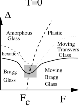
FIG. 17.: Phase diagram in the force $f$, disorder $\Delta$ in $d=3$ at $T=0$. The behaviour in the square region is unclear. An interesting possibility would be a direct depinning of an hexatic into the Moving Transverse glass, but other scenario are possible.

FIG. 18.: Phase diagram in the temperature $T$, disorder $\Delta$ in $d=3$ for a fixed velocity (not too small). This phase diagram is the dynamical version to the static one (containing the Bragg glass, the vortex glass, and the field driven transition). The MBG can either thermally melt (via a first order transition) or decouple because of disorder.

FIG. 19.: Phase diagram in the force $f$, disorder $T$ in $d=3$. The Bragg glass phase also exist at $T=0$ for $f<F_{c}$.

One of the strong features that emerges from this phase diagrams is the fact that the Bragg glass is able to survive motion by turning into the moving bragg glass. On the other hand other, more disordered phases such as the amorphous glass (vortex glass) are likely to be immediately destroyed at finite drive (and finite temperature) and to be continuously related to the liquid.

In d=2, most of the transitions reduce to simple crossover. At $F=0$ and finite disorder dislocations are expected to be present. The resulting phase should thus be continuously connected to the liquid, although it can retain good short distance translational order. At $T=0$ there is a pinned phase until $F_{c}$, which should depin by a plastic flow. At larger drive disorder effects become smaller and one expects the system to revert to a moving glass state. As discussed earlier, due to the presence of disorder induced dislocations, this state is a Moving transverse glass (if $d=2$ is above its lower critical dimension). At any finite temperature, one can use the RG flow of section VII. Since the temperature renormalizes above the melting temperature and disorder flows to zero the resulting phase should be a driven liquid.

FIG. 20.: Phase diagram in the force $f$, disorder $T$ in $d=3$. There will be very long crossover not represented.

G comparison with numerical simulations

Some of the predictions of the Moving Glass theory contained in the short account of our work [68] have been later verified in several numerical simulations in $d=2$ and $d=3$.

The static channels were clearly observed at $T=0$ in $d=2$ [83]. They were also observed in Ref. [85]. The transverse critical force at $T=0$ in $d=2$ was observed very clearly in [83] and in [86] (see also [85]) and found to be a fraction of the longitudinal critical force which is a reasonable order of magnitude. The effect of a non zero temperature $T>0$ was observed to weaken the effect of transverse barriers in [86] in $d=2$. Note that some non linear effects were observed to persist for low enough transverse force and temperature. Such an observation is in agreement in the discussion of Section () and can be interpreted as a long crossover.

Sharp Bragg peaks were observed in the direction transverse to motion in [83] at $T=0$. However the order along the $x$ direction was found to have fast decay. This is consistent with a decoupling of the channels, and the resulting state was termed the “moving transverse glass”. This is consistent with the expectations from the theory presented here, as illustrated on the phase diagram (20). This phase is presumably the $T=0$ moving transverse glass fixed point analyzed in Section () which does have a non zero transverse critical force. This is in fact confirmed by the observation of [86] of a smectic type of order where well separated dislocations exist between the channels consistent with the expectations discussed in Section (). The absence of long range order was also observed in [87] in a stronger disorder situation.

In $d=3$, a simulation of a driven discrete superconducting XY gauge model [88] finds not perfect but still well defined Bragg peaks at $T>0$ (near the melting), a result which indicates that the driven lattice is in a quasi ordered moving Bragg glass state. In another study on the simpler $d=3$ driven XY model at $T=0$ [89], it was found that indeed there is a phase without topological defects at large enough drive. If it carries to the lattice problem it would indicate that indeed there is a $d=3$ moving Bragg glass state.

Finally note that there are also very recent simulations of a lattice with a periodic substrate [90, 50]. This is a simpler case where a transverse critical current exist (it does exist for a single particule). It may be worthile to investigate this case in all details.

All the above numerically observed effects seem to be in qualitative agreement with the predictions in [68]. However, it would be very useful to be able to make a more quantitative comparison. This should now be possible, as we will give here more detailed predictions than the short account [68]. Among the various interetsing topics to check are the algebraic decay of translational order in $d=3$, a detailed study of the dependence of the transverse critical force on the velocity, the exponent $\theta$ of the transverse depinning, a measure of the barriers at low temperatures, a characterization of the history dependence, and zero and at low temperature.

H comparison with experiments

The moving glass picture has also been confronted with experiments. Since these experiments need the characterization of a moving structure they are challenging. The transverse critical current can in principle be observed in transport experiments (and will show up as hysteretic effects). These are difficult though because of dissipation in the longitudinal direction.

Decoration experiments on the moving vortex lattice have been performed recently by Marchevsky et al. [91]. In these experiments the external field is slowly varied and vortices are decorated while they move. The decoration particles thus accumulate on the regions where vortices are flowing preferentially. The lattice is observed to move in the symmetry axis direction and relatively large regions of highly correlated static channels are observed. These channels do not look like “plastic channels” but rather like the channels predicted in [68]. Note however that some dislocations along $y$ appear (defects in the layered structure). This may be due to strong disorder effects or since the advancing front geometry is in the shape of a droplet some dislocations are unavoidable. Another set of experiments in NBSe2 was also reported in [92]. Note that there has also been several decoration experiments performed just after the current is turned off. These can in principle probe the defect structure of the flowing lattice (though one may worry about transient effects) but cannot show the channel structure.

In [68] we have suggested that the transverse barriers may explain the anomalies recently observed in the Hall effect in a Wigner crystal in a constant magnetic field [13, 12].

The qualitative analysis suggested by the moving glass theory is as follows. An electric field $E_{x}$ is applied in along the $x$ direction. The Wigner crystal starts moving along $x$ when the applied field is larger than a “longitudinal” threshold $E_{x}>E_{c}$. It produces a current along $x$, $I_{x}=qv_{x}$ which is directly measured. Below the longitudinal threshold a highly non linear regime is observed where activated motion dominate. Since it is moving in a high magnetic field, the moving Wigner crystal is submitted to a transverse Lorentz force $F^{L}_{y}=qv_{x}B$. The geometry of the experiment is such, however, that no transverse motion is permitted in the stationary state (because of zero current boundary conditions), and thus $v_{y}=0$. Thus the transverse Lorentz force must be balanced by a transverse electric field, which is thus generated, and is measured as the Hall voltage $V_{y}$. In the absence of transverse pinning the Hall voltage is $V_{y}=LBI_{x}$. Remarkably, it is found in the experiment that the actual measured Hall voltage is indeed $V_{y}=LBI_{x}$ for small $I_{x}$, then experiences a plateau, and finally starts again growing linearly with a slope $dV_{y}/dI_{x}\approx LB$. We have interpreted the different behaviours upon increase of $I_{x}$ as follows. For small $I_{x}$ one is near the longitudinal depinning and it is probably a plastic flow regime with little transverse barriers. Then upon motion, a transition to a moving solid occurs, which is presumably a moving glass. The existence of a non zero transverse critical force $F^{c}_{y}>0$ then immediately implies that there are sliding states with $v_{y}=0$ as long as $F^{L}_{y}<F^{c}_{y}$ and no Hall voltage necessary.

Finally note a recent experiment [93] on superconducting multilayers where it was found that the flux flow resistivity exhibit quasi periodic oscillations as a function of the field. This was interpreted [93] in terms of dynamics matching of the moving vortex lattice with the periodic substrate. This is compatible with the presence of a quasi ordered structure in motion.

It would be interesting to probe further the channel structure by direct imaging techniques. In particular one may investigate the degree of reproducibility of the channel pattern. It is predicted that upon sudden reversal of the velocity the channels should be different. The question of order and quasi order can be probed in experiments such as neutron scattering, flux lattice imaging magnetic noise experiments, NMR experiments and more indirectly in transport measurements. Other imaging techniques such as $\mu$-SR NMR electron holography can also be used. Finally it would be interesting to check for similar effects in the presence of columnar defects since, as discussed in this paper we predict the formation of a moving Bose glass.

IV The Model and Physical Content

A Derivation of the equations of motion

Let us first derive the equation of motion for a lattice submitted to external force $f$. We work in the laboratory frame. This offers several advantages that will become obvious later. We denote by $R_{i}(t)$ the true position of an individual vortex in the laboratory frame. The lattice as a whole moves with a velocity $v$. We thus introduce the displacements $R_{i}(t)=R_{i}^{0}+vt+u_{i}(t)$ where the $R_{i}^{0}$ denote the equilibrium positions in the perfect lattice with no disorder. $u_{i}$ represent the displacements compared to a moving perfect lattice (and corresponds to the position of the i-th particle in the moving frame). The definition of $v$ imposes $\sum_{i}u_{i}(t)=0$ at all times. We furthermore assume that the motion is overdamped. The exact equation of motion can then be obtained from the Hamiltonian $H$ by

$$\eta\frac{du_{i}(t)}{dt}=-\frac{\delta H}{\delta u_{i}}+f-\eta v+\zeta_{i}(t)$$ (27)

where $\eta$ is the friction coefficient and the thermal noise satisfies $\overline{\zeta_{i}(t)\zeta_{j}(t)}=2T\eta\delta_{ij}\delta(t-t^{\prime})$. The Hamiltonian is the standard Hamiltonian for periodic structure in a random potential $H=H_{\text{el}}+H_{\text{dis}}$. $H_{\text{el}}$ is the standard elastic Hamiltonian, and $H_{\text{dis}}$ describes the interaction with the random potential

$$H_{\text{dis}}=\int_{r}V(r)\rho(r)=\sum_{i}\int_{r}V(r)\delta(r-R_{i}^{0}+vt+u_{i}(t))$$ (28)

where the random potential has correlations $\langle V(r)V(r^{\prime})\rangle=g(r-r^{\prime})$ of range $r_{f}$.

In order to use the standard field description of the displacement $u$ instead of focussing on the equation for one particle, one rewrites (27) as

$$\eta\frac{du_{i}(t)}{dt}=-\frac{\delta H_{el}}{\delta u_{i}}+\int_{r}\partial V(r)\delta(r-R_{i}^{0}+vt+u_{i}(t))+f-\eta v+\zeta(R_{i}(t),t)$$ (29)

In doing so one would get the same thermal noise for two particles being at the same place at the same time, instead of the two independent noises of equation (27). Since such a configuration cannot happen, going from (27) to (29) is essentially exact.

As for the static case [38, 39] the difficulty is to take the continuum limit of (29) since the disorder can vary at a much shorter scale than the lattice spacing $a$. To proceed one follows the same steps than for the static case, suitably modified to take into account the time dependence of the displacements. One first introduces a smooth interpolating displacement field $u(r,t)$ such that $u(R_{i}^{0}+vt,t)=u_{i}(t)$ (see formula $A2$ of [38, 39]). The field $u(r,t)$ is the smoothest field interpolating between the actual positions $u_{i}(t)$. All coordinates $r$ are expressed in the laboratory frame. The field $u(r,t)$, whose components we denote by $u_{\alpha}(r,t)$ thus expresses the displacement in the moving frame, as a function of the coordinates of the laboratory frame.

As for the static, if one assumes the absence of dislocations at all times the particles can be labeled in a unique way. One then introduces the continuous labelling field:

$$\phi(r,t)=r-vt-u[\phi(r,t)+vt,t]$$ (30)

Thus $\phi(R_{i}(t),t)=\phi(R_{i}^{0}+vt+u_{i}(t),t)=R_{i}^{0}$ by definition, and $\phi$ numbers the particles by their initial positions. In the absence of dislocations the field $\phi(r,t)$ is uniquely defined.

To obtain the continuum limit of the equation (29) one first performs the continuum limit in the Hamiltonian as in [39], to obtain for the disorder term

$$H_{\text{pin}}=\int dxV(x)\rho(x)=-\rho_{0}\int dxV(x)\partial_{\alpha}u_{\alpha}+\rho_{0}\int dx\sum_{K\neq 0}V(x)e^{iK\cdot(r-vt-u(r,t))}$$ (31)

where $K$ spans the reciprocal lattice and $\rho_{0}$ is the average density.

In (31) we have made the approximation

$$u(\phi(r,t)+vt,t)\sim u(r,t)$$ (32)

Such an approximation is exact up to higher powers of $\partial u$, negligeable in the elastic limit, as for the static case [39]. However the dynamic case is more subtle since such terms could generate when combined with a non-zero velocity relevant terms. This is the case for example of the so-called KPZ terms generated through cutoff effects. Since it is hopeless to try to tackle from first principle all such additional terms the only safe procedure is to assume that every term allowed by symetry will be generated, and has to be examined. We will proceed with such a program in section VIII B. For the moment we only retain the dominant terms of (31). If one then takes the derivative with respect to the smooth field $u(r,t)$ one obtains for the equation of motion in the laboratory frame

$$\eta\partial_{t}u_{rt}^{\alpha}+\eta v\cdot\nabla u_{rt}^{\alpha}=\int_{r^{\prime}}\Phi_{\alpha\beta}(r-r^{\prime})u_{rt^{\prime}}^{\beta}+F_{\text{pin}}^{\alpha}(r,t)+f_{\alpha}-\eta v_{\alpha}+\zeta_{\alpha}$$ (33)

where $\Phi_{\alpha\beta}(r-r^{\prime})$ is the elastic matrix. The term $\eta v\cdot\nabla u_{\alpha}$ comes from the standard Euler representation when expressing the displacement field in the laboratory frame. $-\eta v_{\alpha}$ is the average friction and in the continuum $v$ is determined by the condition that the average of $u$ is zero. The thermal noise satisfies in the continuum limit

$$\overline{\zeta_{\alpha}(r,t)\zeta_{\beta}(r^{\prime},t^{\prime})}=2T\eta\delta_{\alpha\beta}\delta^{d}(r-r^{\prime})\delta(t-t^{\prime})$$ (34)

and

$$F^{\text{pin}}_{\alpha}(r,t)=-\delta{H_{\text{pin}}}/\delta u_{\alpha}(r,t)=V(r)\rho_{0}\sum_{K}iK_{\alpha}\exp(iK\cdot(r-vt-u(r,t)))-\rho_{0}\nabla_{\alpha}V(r)$$ (35)

is the pinning force. Note the difference between our equation (33) and the one derived in [65], which does not contain the convective term. This difference comes simply from a different definition of the displacement fields. They consider displacements fields labelled by the original position of the particle (i.e. the actual position of the particle is $r+u$) whereas for us $r$ denotes the actual position of the vortex considered (i.e. in the presence of an external potential $V$ the potential acting on the vortex at point $r$ is $V(r)$ instead of $V(r+u)$ for [65]).

In Appendix A we give a more general derivation of (35) valid even for cases where the equation of motion is not the derivative of a potential.

B Models and Symmetries

Before we even attempt to solve (33), let us examine the various symmetries of the problem and define several models which approximate the physical problem at various levels.

The physical symmetry of the original equation of motion (27) is the global inversion symmetry ($r\to-r$, $u\to-u$, $v\to-v$ $f\to-f$). When the force (and thus $v$) is along a principal lattice direction, one has then two independent inversion symmetries $I_{x}=$ ($x\to-x$, $u_{x}\to-u_{x}$, $v\to-v$ $f\to-f$) and $I_{y}=$ ($y\to-y$, $u_{y}\to-u_{y}$). These symmetries are exact and hold in all cases. They are the only symmetries of the original model (27). The proper continuum limit of equation (27) must thus include all terms which are relevant and consistent with these exact symmetries. We define such a model as Model I, which will be studied in more details in Section (VIII B). The additional terms can originate from e.g anharmonic elasticity, cutoff effects or higher order terms in $\nabla u$, as will be dicussed in Section VIII B.

If one drop in Model I the terms which are small in the elastic limit $\nabla u\ll 1$, one obtains another model that we call Model II. It corresponds to the continuum limit of the equation of motion to obtain equation (33) i.e. (33) in the elastic limit. Although model II is slightly simpler than model I, it only misses terms which are small in the bare equation but would be allowed by the above symmetries. Even if some of them are relevant, the would only be able to change the physics compared to model II at very large length scales. One thus expects model II to give in practice an extremely accurate description of the physics.

The Model II posesses a higher symmetry than Model I: let us examine the symmetries of the pinning force (35). Using the correlator of the random potential $V$, the correlator of the pinning force is:

$$\Delta_{\alpha\beta}=\overline{F^{\text{pin}}_{\alpha}(r,t,u_{rt})F^{\text{pin}}_{\beta}(r^{\prime},t^{\prime},u_{r^{\prime}t^{\prime}})}=\rho_{0}^{2}g(r-r^{\prime})\sum_{K,K^{\prime}\neq 0}iK_{\alpha}iK^{\prime}_{\beta}e^{iK\cdot(r-vt-u_{rt})+iK^{\prime}\cdot(r^{\prime}-vt^{\prime}-u_{r^{\prime}t^{\prime}})}$$ (36)

Since $u$ is a smooth field it has no rapidly oscillating components and thus in (36) the terms that are rapidly oscillating in $r+r^{\prime}$ can be discarded. Setting $K^{\prime}=-K$ in (36), one is left with

$$\Delta_{\alpha\beta}=\rho_{0}^{2}\sum_{K\neq 0}K_{\alpha}K_{\beta}g(r-r^{\prime})\exp(iK\cdot(r-r^{\prime})-iK\cdot(u_{rt}-u_{r^{\prime}t^{\prime}}+v(t-t^{\prime}))$$ (37)

The symmetries of (37) thus a priori depends on the precise form of the correlator $g(r)$. However in the elastic limit it is legitimate to replace $u_{r^{\prime}t^{\prime}}$ by $u_{rt^{\prime}}$ in the above expression. Integrating then over $r^{\prime}$ one obtains:

$$\Delta_{\alpha\beta}=\rho_{0}^{2}\sum_{K\neq 0}K_{\alpha}K_{\beta}g_{K}\exp(-iK\cdot(u_{rt}-u_{rt^{\prime}}+v(t-t^{\prime}))$$ (38)

where $g_{K}$ is the Fourier coefficient of the correlator $g(r)$. Since $g_{K}$ is essentially zero for $K\gg 1/r_{f}$, the error made in the above approximation is itself of order $\nabla u$ and thus consistent with the elastic limit approximation. This justifies the choice of (38) as the random force correlator in Model II. The disorder term then posseses the statistical tilt symmetry (STS) $u_{rt}\to u_{rt}+f(r)$ where $f(r)$ is an arbitrary function. In this case one can absorb any static change in $u$ without affecting the correlations of the pinning force. Furthermore in the case of isotropic elasticity, the additional inversion symmetry $y\to-y$ holds.

Though we will study the complete Model II in Sections V and VIII B its main physics can be understood[68] by noticing that the pinning force $F^{\text{pin}}_{\alpha}(r,t)$ in (35) naturally splits into a static and a time-dependent part:

$$F_{\alpha}^{\text{stat}}(r,u) = V(r)\rho_{0}\sum_{K.v=0}iK_{\alpha}\exp(iK\cdot(r-u))-\rho_{0}\nabla_{\alpha}V(r)$$ (39)

$$F_{\alpha}^{\text{dyn}}(r,t,u) = V(r)\rho_{0}\sum_{K.v\neq 0}iK_{\alpha}\exp(iK\cdot(r-vt-u))$$ (40)

The static part of the random force comes from the modes such that $K.v=0$ which exist for any direction of the velocity commensurate with the lattice. The maximum effect is obtained for $v$ parallel to one principal lattice direction, the situation we study now. This force originates only from the periodicity along $y$ and the uniform density modes along $x$, i.e the smectic-like modes. Since this static pinning force $F_{\alpha}^{\text{stat}}(r,u)$ is along the $y$ direction, it is useful consider only the transverse part (along $y$) of the equation of motion (33) dropping $F_{\alpha}^{\text{dyn}}$. This leads to introduce Model III, defined by the following equation of motion in the laboratory frame:

$$\eta\partial_{t}u_{y}+\eta v\partial_{x}u_{y} = c\nabla^{2}u_{y}+F^{\text{stat}}(r,u_{y}(r,t))+\zeta_{y}(r,t)$$ (41)

$$F^{\text{stat}}(x,y,u_{y}) = V(x,y)\rho_{0}\sum_{Ky\neq 0}K_{y}\sin{K_{y}(u_{y}-y)}-\rho_{0}\partial_{y}V(r)$$ (42)

Although for non isotropic elasticity $u_{x}$ also appears in the equation of motion for $u_{y}$, and can in principle lead to additional static effects, it is not included in Model III for reasons which will be explained below. Thus Model III only involves the transverse displacements $u_{y}$. It posesses the same symmetries as Model II with the three additional independent symmetries $y\to-y$, $u_{y}\to-u_{y}$ and ($x\to-x$, $v\to-v$) and is also defined in the elastic limit.

It is to be emphasized that although the derivation of model III was given here systematically starting from an elastic description. the only serious hypothesis behind Model III is the existence of transverse periodicity [94]. As discussed in section II B (42) will be the correct starting point to describe any kind of structure have such transverse periodicity properties. One thus expects model III to be the generic equation containing the physics necessary to describe these structures.

V Perturbation theory for the complete time-dependent equation

Let us start by a simple perturbation analysis of the equation of motion Model II. Such a large velocity or weak disorder expansion has a long history in various contexts such as vortex lattices [66, 65] and charge density waves [27, 95]. The natural idea is that at large velocity the disorder term oscillates rapidly and averages to a small value and that $1/v$ is a good expansion parameter. As we will see such an idea is in fact incorrect, since previously unnoticed divergences appear in the perturbation theory.

A Analysis to first order

We start from the initial equation (33) defining Model II that we rewrite as:

$${(R^{-1})}^{\alpha\beta}_{rtr^{\prime}t^{\prime}}u^{\beta}_{r^{\prime}t^{\prime}}=f_{\alpha}-\eta_{\alpha\beta}v_{\beta}+f_{\alpha}(r,t,u_{rt})$$ (43)

where from now on we drop the pin subscript on $f$. The response kernel $R$ is defined in Fourier space:

$${(R^{-1})}^{\alpha\beta}_{qt,q^{\prime}t^{\prime}}=\delta_{tt^{\prime}}\delta_{q^{\prime},-q}(\eta_{\alpha\beta}\partial_{t}+i\eta_{0}v_{\gamma}q_{\gamma}\delta_{\alpha\beta}+C_{T}(q)P^{T}_{\alpha\beta}(q)+C_{L}(q)P^{L}_{\alpha\beta}(q))$$ (44)

where the elastic matrix is : $C_{T}(q)=c_{66}q^{2}$, $C_{L}(q)=c_{11}q^{2}$ for a two dimensional problem and $C_{T}(q)=c_{66}q^{2}+c_{44}q_{z}^{2}$, $C_{T}(q)=c_{11}q^{2}+c_{44}q_{z}^{2}$ for a three dimensional problem. The bare value of the friction coefficient $\eta_{0}$ is defined as $\eta_{\alpha\beta}=\delta_{\alpha\beta}\eta_{0}$. In (43) the velocity is fixed by the constraint that $\langle u^{\beta}\rangle=0$ to all orders in perturbation theory. This is equivalent to enforce that the linear term in the effective action [96] is exactly zero.

Instead of working directly with the equation of motion it is more convenient to use the Martin-Siggia-Rose formalism [97]. The generic de Dominicis-Janssen MSR functional is given by

$$Z[h,\hat{h}]=\int DuD\hat{u}e^{-S[u,\hat{u}]+\hat{h}u+ih\hat{u}}$$ (45)

where $\hat{h},h$ are source fields. The MSR action corresponding to the equation of motion (43) and the disorder correlator (38) is

$$S[u,\hat{u}]=S_{0}[u,\hat{u}]+S_{int}[u,\hat{u}]$$ (46)

with

$$S_{0}[u,\hat{u}] = \int_{rtr^{\prime}t^{\prime}}~{}i\hat{u}^{\alpha}_{rt}(R^{-1})^{\alpha\beta}_{rt,r^{\prime}t^{\prime}}u^{\beta}_{r^{\prime}t^{\prime}}-i\hat{u}^{\alpha}(f_{\alpha}-\eta_{\alpha\beta}v_{\beta})-\eta T\int_{r,t}(i\hat{u}^{\alpha}_{rt})(i\hat{u}^{\alpha}_{rt})$$ (47)

$$S_{int}[u,\hat{u}] = -\frac{1}{2}\int drdtdt^{\prime}(i\hat{u}^{\alpha}_{rt})(i\hat{u}^{\beta}_{rt^{\prime}})\Delta^{\alpha\beta}(u_{rt}-u_{rt^{\prime}}+v(t-t^{\prime}))$$ (48)

Note that (46) corresponds to the action derived in Appendix A.

The fundamental functions to compute are the disorder averaged displacements correlation function $C^{\alpha,\beta}_{rt,r^{\prime}t^{\prime}}=\overline{\langle u^{\alpha}_{rt}u^{\beta}_{r^{\prime}t^{\prime}}\rangle}$ and the response function $R^{\alpha,\beta}_{rt,r^{\prime}t^{\prime}}=\delta\overline{\langle u^{\alpha}_{rt}\rangle}/\delta h^{\beta}_{r^{\prime}t^{\prime}}$ which measures the linear response to a perturbation applied at a previous time. They are obtained from the above functional as $C^{\alpha\beta}_{rt,r^{\prime}t^{\prime}}=\langle u^{\alpha}_{rt}u^{\beta}_{r^{\prime}t^{\prime}}\rangle_{S}$ and $R^{\alpha\beta}_{rt,r^{\prime}t^{\prime}}=\langle u^{\alpha}_{rt}i\hat{u}^{\beta}_{r^{\prime}t^{\prime}}\rangle_{S}$ respectively. Causality imposes that $R_{rt,r^{\prime}t^{\prime}}=0$ for $t^{\prime}>t$ and we use the Ito prescription for time discretization which imposes that $R_{rt,r^{\prime}t}=0$. We assume here time and space translational invariance and denote indifferently $C_{rt,r^{\prime}t^{\prime}}=C_{r-r^{\prime},t-t^{\prime}}$ and $R_{rt,r^{\prime}t^{\prime}}=R_{r-r^{\prime},t-t^{\prime}}$ by the same symbol, as well as their Fourier transforms when no confusion is possible. Note that in this problem $C_{-r,t}\neq C_{r,t}$ when $v$ is non zero. In the absence of disorder the action is simply quadratic $S=S_{0}$. The response and correlation fucntion in the absence of disorder are thus (for $t>0$) and introducing the mobility $\mu=1/\eta$:

$$R^{\alpha\beta}_{q,t}=P^{L}_{\alpha\beta}(q)\mu e^{-(c_{L}(q)+ivq_{x})\mu t}\theta(t)+P^{T}_{\alpha\beta}(q)\mu e^{-(c_{T}(q)+ivq_{x})\mu t}\theta(t)$$ (49)

$$C^{\alpha\beta}_{q,t}=P^{L}_{\alpha\beta}(q)\frac{T}{c_{L}(q)}e^{-(c_{L}(q)\mu|t|+ivq_{x}\mu t)}+P^{T}_{\alpha\beta}(q)\frac{T}{c_{T}(q)}e^{-(c_{T}(q)\mu|t|+ivq_{x}\mu t})$$ (50)

Note that the fluctuation dissipation theorem (FDT)

$$TR^{\alpha\beta}_{r,t}=-\theta(t)\partial_{t}C^{\alpha\beta}_{r,t}$$ (51)

does not hold here (it holds only for $v=0$) since we are studying a moving system which does not derive from a Hamiltonian.

It is easy to show that the disorder does not produce any correction to the part $i\hat{u_{t}}(cq^{2}+ivq_{x})u_{t}$ of the action, and thus that the parameters $c$ ($c_{11}$ and $c_{66}$ ) and $\eta_{0}v$ are not renormalized (we consider here for simplicity the isotropic version $c=c_{11}=c_{66}$ but this property holds in general). This is similar to the property of non renormalization of connected correlations in the statics (for $v=0$) due to the statistical tilt symmetry. Indeed here one has the exact relation:

$$\overline{\log Z[h_{t},\hat{h}]}=-\int dt~{}h_{t}(cq^{2}+ivq_{x})^{-1}\hat{h}+\overline{\log Z[h_{t},0]}$$ (52)

where $\hat{h}$ is an arbitrary static field. This relation implies that the static response function $\int dt^{\prime}R_{q,t,t^{\prime}}=(cq^{2}+ivq_{x})^{-1}$ is not renormalized. The property (52) is demonstrated by performing the change of variable $u_{t,r}=u^{\prime}_{t,r}+f_{r}$ with $f_{q}=-(cq^{2}+ivq_{x})^{-1}\hat{h}_{q}$ in the action and noticing that the change in the random force $F(r,u)\to F^{\prime}(r,u)=F(r,u+f)$ is thus that all averages over $F$ and $F^{\prime}$ are identical since they have the same correlator from (38).

Let us now study the perturbation theory in the disorder and compute the effective action $\Gamma[u,\hat{u}]$ to lowest order in the interacting part $S_{int}$, using a standard cumulant expansion

$$\Gamma[u,\hat{u}]=S_{0}[u,\hat{u}]+\langle S_{int}[u+\delta u,\hat{u}+\delta\hat{u}]\rangle_{\delta u,\delta\hat{u}}$$ (53)

where the averages in (B1) over $\delta u$, $\delta\hat{u}$ are taken with respect to $S_{0}$.

The calculations are performed in Appendix B. One finds that the effective action has the same form as the bare action, up to irrelevant higher order derivative terms, with the following modifications. First the full non linear form of the correlator of the pinning force is corrected by thermal fluctuations $\Delta^{\alpha\beta}_{K}\to\tilde{\Delta}^{\alpha\beta}_{K}$. In $d>2$ it reads:

$$\tilde{\Delta}^{\alpha\beta}_{K}=\Delta^{\alpha\beta}_{K}e^{-\frac{1}{2}K^{2}B_{\infty}}$$ (54)

or equivalently $\tilde{g}_{K}=g_{K}e^{-\frac{1}{2}K^{2}B_{\infty}}$ where $B_{\infty}=\langle u^{2}\rangle_{th}$. We have defined $B^{\alpha\beta}_{r,t}=2(C^{\alpha\beta}_{0,0}-C^{\alpha\beta}_{r,t})$. This amounts to a smoothing out of the disorder by thermal fluctuations. Secondly, the friction coefficient matrix is corrected by $\delta\eta_{\alpha\beta}$, and the temperature by $\delta T$. Finally, the driving force is corrected by $\delta f$ (we are working at fixed velocity, enforcing order by order that $f+\delta f=\eta v$).

Let us start by the corrections to the driving force. We find:

$$\delta f_{\alpha}(v)=\sum_{K}\sum_{I=L,T}\int_{BZ}dqK_{\alpha}(K.P^{I}(q).K)g_{K}\frac{v.(K+q)}{c_{I}(q)^{2}+(\eta_{0}v.(K+q))^{2}}$$ (55)

To derive this formula from (LABEL:correction1) we have used the symmetry $K\to-K$. This formula gives the lowest correction to the driving force at fixed velocity or, equivalently to the velocity at fixed driving force. It is identical to the formula (22) of Schmidt and Hauger [66]. There are small differences, unimportant in the elastic limit, which come from the different definitions of the continuum limit of the model (see discussion in section IV A).

A salient feature of the above formula was noticed by Schmidt and Hauger, i.e the velocity and the force are not, in general, aligned. There are aligned however when the velocity is along one of the principal lattice directions, i.e $K_{0}.v=0$ where $K_{0}$ is one of the principal reciprocal lattice vector (note that this is also the case for the median direction $\pi/6$). Such a feature is reasonable on physical grounds and can be confirmed by higher order analysis of the perturbation theory (see section VI).

Furthermore, using the approximation $v(K+q)\sim vK$ Schmidt and Hauger found that, in $d=2$, the transverse pinning force versus the angle $\alpha$ between the velocity and one principal direction of the lattice has a discontinuity at $\alpha=0$. One could naively think that such a discontinuity could be interpreted as the existence of a transverse critical current. Indeed a natural interpretation of figure 1 of [66] would be that one need to apply a finite force to the lattice (opposite to the transverse pinning force) to tilt sightly its velocity from the principal axis direction. Notable confusion on this subject existed at that time in the litterature [66, 65]. Such an interpretation is in fact incorrect. First, as Schmidt and Hauger correctly pointed out such a discontinuity is an artefact of the approximation $v(K+q)\sim vK$, and diseappears if the correct expression (55) is used. Furthermore it is easy to check that even with the above approximation the discontinuity exists only in $d=2$ and the function is continuous for $d>2$. Thus the first order perturbation does not exhibit any divergence and does not give rise to a transverse critical current.

In order to have divergences in the perturbation theory (and the associated effects) it is thus necessary to examine the perturbation theory to second. We will perform such a calculation in section VI.

Before we do so it is interesting to examine the first order corrections to the friction coefficient and the temperature.

$$\delta\eta_{\alpha\beta}(v)=\int_{rt}tR^{\gamma\delta}_{r=0,t}K_{\gamma}K_{\beta}\Delta^{\alpha\delta}_{K}e^{-iK.vt}e^{-\frac{1}{2}K.B_{0,t}.K}$$ (56)

At zero temperature it reads:

$$\delta\eta^{\alpha\beta}(v)=-\int d\tau dr\tau R^{\gamma\delta}(r=0,\tau)\Delta^{\alpha\delta;\gamma\beta}(v\tau)$$ (57)

Still at $T=0$ and using the bare form of the disorder one finds:

$$\delta\eta_{\alpha\beta}=\sum_{K}\sum_{I=L,T}\int_{BZ}dqK_{\alpha}K_{\beta}(K.P^{I}(q).K)g_{K}\frac{1}{(c_{I}(q)+i\eta_{0}v.(K+q))^{2}}$$ (58)

When the velocity is along a principal lattice direction one finds that $\delta\eta_{xy}=0$ and thus the friction matrix remains diagonal. However the corrections to the friction is clearly not the same along $x$ and $y$.

Next we give the corrections to temperature. They are:

$$\delta(\eta T)_{\alpha\beta}=\frac{1}{2}\sum_{K}\int_{t}\Delta^{\alpha\delta}_{K}e^{-iK.vt}(e^{-\frac{1}{2}K.B_{0,t}.K}-e^{-\frac{1}{2}K.B_{\infty}.K})$$ (59)

Contrarily ot the velocity corrections, corrections to the temperature (59) exhibit divergences for any $v$ already at the first order in the disorder. However these divergences are well hidden and can only appear if one looks at the non zero temperature perturbation theory, which was not done in [65, 66]. At $T=0$ one finds trivially that $\delta T=0$, showing that disorder alone cannot generate a finite temperature. Such corrections are thus non trivial and there is in general no simple relation between $\delta(\eta T)_{\alpha\beta}$ and $\delta(\eta)_{\alpha\beta}$, due to the absence of FDT theorem. Only in the particular case where $v=0$ and of potential random forces $\Delta^{\alpha\delta}_{K}=K_{\alpha}K_{\beta}g_{K}$ the FDT theorem enforces $\delta T=0$ (see, e.g (51) and [98]). The way to treat these divergences will be examined together with the second order in perturbation in section VI.

B Correlation functions

The last physical information that can be extracted from the perturbation theory is about the correlation functions. The calculation is performed in appendix B, and this gives (see (LABEL:corrtfin)) in the static limit (see (LABEL:corrtfin) for the full expresion)

$$\overline{\langle u^{\alpha}_{-q}u^{\beta}_{q}\rangle} = \sum_{K,K.v=0}\sum_{I=L,T,I^{\prime}=L,T}\int_{BZ}dq(2\pi)g_{K}\frac{P^{I}_{\alpha\gamma}(q)}{c_{I}(q)+i\eta_{0}v.q}\frac{P^{I^{\prime}}_{\beta\delta}(q)}{c_{I}^{\prime}(q)-i\eta_{0}v.q}D_{\gamma\delta}$$ (60)

where the disorder is renormalized by the temperature

$$g_{K}D_{\gamma\delta}(\omega)=g_{K}K_{\gamma}K_{\delta}e^{-\frac{1}{2}K.B_{0,\infty}.K}$$ (61)

Let us first focuss on the $T=0$ limit of (60). The length $R_{c}^{x,y}$ can be estimated by looking at $A=\overline{\langle u^{x}_{-q}u^{x}_{q}+u^{y}_{-q}u^{y}_{q}\rangle}$. This gives

$$A=\sum_{K,K.v=0}\int_{BZ}dq(2\pi)K_{y}^{2}\left[\frac{q_{x}^{2}}{q_{\perp}^{2}(v^{2}q_{x}^{2}+(c_{66}(q_{x}^{2}+q_{y}^{2})+c_{44}q_{z}^{2})^{2})}+\frac{q_{y}^{2}}{q_{\perp}^{2}(v^{2}q_{x}^{2}+(c_{11}(q_{x}^{2}+q_{y}^{2})+c_{44}q_{z}^{2})^{2})}\right]$$ (62)

where $q_{\perp}^{2}=q_{x}^{2}+q_{y}^{2}$. Since $q_{x}\sim q_{y}^{2}$ one immediately sees from (62) that the compression modes are the one responsible for the divergences. Other modes are not divergent around $d=3$. Lengthscqles $R_{c}$ qre theus controled by $c_{11}$.

On the other hand in order to obtain a decoupling of the channels one can use a simple Lindermann criterion.

$$\overline{\langle[u_{x}(y=a)-u_{x}(0)]^{2}\rangle}=C_{L}^{2}a^{2}$$ (63)

Using (60) one gets

$$B_{xx}(y=a)\approx\Delta_{yy}\int_{q,BZ}\frac{q_{x}^{2}}{q_{\perp}^{2}(v^{2}q_{x}^{2}+(c_{66}(q_{x}^{2}+q_{y}^{2})+c_{44}q_{z}^{2}))}$$ (64)

we have neglected all terms containing $c_{11}$. One can thus neglect the compression mode. The decoupling between the channels is thus controled by $c_{66}$ whereas the roughness of the channels and the characteristics lengthcales of the moving glass will directly depend on the compression mode $c_{11}$. Estimating the integral one finds in $d=3$:

$$B_{xx}(y=a)\sim\frac{\Delta_{yy}}{a^{2}c_{44}^{1/2}}\min((\frac{a^{2}}{c_{66}})^{3/2},(a/v)^{3/2})$$ (65)

One recovers the Bragg glass estimate (in the simpler case $a=r_{f}$).

The above perturbation expansion for the Lindemann criterion implicitely supposes that the random force is directed along the $y$ direction. In fact, under renormalization a random force along $x$ is also generated as discussed in section III. One can use again the Lindemann criterion with a random force along $x$. In that case only the transverse modes remain are important (fo small enough $q_{x}$).

VI Renormalization group study of the transverse physics (moving glass)

Up know we have studied the perturbation expansion of the full continuous model II, keeping both the $x$ and $y$ directions. Doing the second order perturbation on that full model is tedious. Since one knows on physical grounds that the singularities in the perturbation theory will come from the static components of the disorder [68] , which as was discussed in Section II B originate from the transverse degrees of freedom, we now study the perturbation theory of the simplified transverse equation of motion, Model III. If, as we indeed find, this perturbation theory is singular, this implies divergences in the full model II as well. Model III will thus give a good description of the physics. We thus study it here and come back to the full Model II in the next Section  VIII A.

A zero temperature perturbation theory to second order

To avoid cumbersome expressions, and since in this whole section we only discuss transverse degrees of freedom we skip the index $y$ for $u_{y}$. We also discuss here for simplicity a $n=1$ component model for the transverse displacement $u$ (which is appropriate for flux lines in $d=3$ and point vortices in $d=2$). Generalizations to $n>1$ will be briefly mentionned in Section VI D.

We thus study the dynamical equation for Model III [68]. Since we will be dealing with an anisotropic fixed point it is useful to distinguish $c_{x}$ and $c_{y}$.

$$\eta\partial_{t}u_{rt}=(c_{x}\nabla_{x}^{2}+c_{y}\nabla_{y}^{2}-v\partial_{x})u_{rt}+F(r,u_{rt})+\zeta(r,t)$$ (66)

The bare value of the friction coefficient along $y$ is denoted by $\eta_{0}$, and for simplicity we denote by $v$ the quantity $\eta_{0}v$ (which remains uncorrected to all orders in this model). The correlator of the static transverse pinning force is (42):

$$\overline{F(r,u)F(r^{\prime},u^{\prime})}=\Delta(u-u^{\prime})\delta^{d}(r-r^{\prime})$$ (67)

Averages over solutions of (66) can be performed using the Martin-Siggia-Rose (MSR) action:

$$Z[h,\hat{h}] = \int DuD\hat{u}e^{-S_{0}[u,\hat{u}]-S_{int}[u,\hat{u}]+hu+i\hat{h}\hat{u}}$$ (68)

$$S_{0}[u,\hat{u}] = \int_{rt}~{}i\hat{u}_{rt}(\eta\partial_{t}+v\partial_{x}-c_{x}\nabla_{x}^{2}-c_{y}\nabla_{y}^{2})u_{rt}-\eta T(i\hat{u}_{rt})(i\hat{u}_{rt})$$ (69)

$$S_{int} = -\frac{1}{2}\int_{rtt^{\prime}}(i\hat{u}_{rt})(i\hat{u}_{rt^{\prime}})\Delta(u_{rt}-u_{rt^{\prime}})$$ (70)

In this section we will restrict ourselves to $T=0$. The corrections coming from correlation functions $\langle\delta u_{t}\delta u_{t^{\prime}}\rangle\sim T$ then vanish, which simplify the analysis. This can be used to show that to all orders the temperature remains zero. The first order corrections where computed in the Section LABEL:timedependentpt. At $T=0$ there is no correction to the disorder term (to this order). There is a non trivial correction to the kinetic term, which gives the following correction to the friction coefficient $\eta$:

$$\delta\eta=-\Delta^{\prime\prime}(0)\int_{q}\int_{0}^{+\infty}dttR(q,t)$$ (71)

This leads to:

$$\frac{\delta\eta}{\eta}=-\Delta^{\prime\prime}(0)\int\frac{d^{d-1}q_{y}}{(2\pi)^{d-1}}\frac{2c_{x}}{(4c_{x}c_{y}q_{y}^{2}+v^{2})^{3/2}}$$ (72)

(check) This is not a divergent integral, except when $v=0$. To find divergences in the perturbation theory at $T=0$ one has to go to second order.

The second order corrections to the effective MSR action, and thus to the coarse grained equation of motion, are computed in Appendix C. To second order a correction to the full nonlinear disorder correlator appears and reads:

$$\delta\Delta(u)=\Delta^{\prime\prime}(u)(\Delta(0)-\Delta(u))\int_{r}G(r)G(r)-\Delta^{\prime}(u)^{2}\int_{r}G(r)G(-r)$$ (73)

where $G(r)$ is the static response function

$$G(r)=\int_{0}^{\infty}dtR(r,t)\qquad,\qquad G(q)=\frac{1}{c_{x}q_{x}^{2}+c_{y}q_{y}^{2}+ivq_{x}}$$ (74)

At zero velocity both terms in (73) are infrared divergent for $d\leq 4$, as is well known leading to the glassy effects in the statics. The key novelty with respect to the problem at $v=0$ is that due to the assymetry introduced by motion, $G(r)$ is different from $G(-r)$. As a consequence the second term in (73) is now convergent for $v>0$. Indeed the integral

$$\int_{r}G(r)G(-r)=\int_{q}G(q)^{2}=\int\frac{d^{d-1}q_{y}}{(2\pi)^{d-1}}\frac{2c_{x}}{(4c_{x}c_{y}q_{y}^{2}+v^{2})^{\frac{3}{2}}}$$ (75)

is convergent in all dimensions for $v>0$. On the other hand, one divergence remains from the first term:

$$\int_{r}G(r)G(r)=\int_{q}G(q)G(-q)=\int\frac{d^{d-1}q_{y}}{(2\pi)^{d-1}}\frac{1}{2c_{y}q_{y}^{2}\sqrt{4c_{x}c_{y}q_{y}^{2}+v^{2}}}\sim\int\frac{d^{d-1}q_{y}}{(2\pi)^{d-1}}\frac{1}{2vc_{y}q_{y}^{2}}$$ (76)

The integral (76) is divergent for $d\leq 3$, even for $v>0$. Thus, contrarily to general belief [65, 66, 67] originating mainly form the study of the first order perturbation in $1/v$, analysis to second order confirms the surprising conclusion that even at large velocity infrared divergences occur in the perturbation theory [68, 99]. Such divergences indicates the instability of the zero disorder fixed point and the breakdown of the large $v$ expansion. They lead the system to a novel fixed point where the disorder is plays a crucial role. The above divergence is the key to the physics of the moving glass.

B Renormalization group study at zero temperature

In order to handle these new divergences, and to find the new fixed point which describes the large scale physics, we use a dynamical functional renormalization group (DFRG) procedure on the effective action using a Wilson scheme. This allows to keep track of the full function $\Delta(u)$, which is necessary since the full function is marginal at the upper critical dimension. This is equivalent to decompose the fields into fast and slow components $u\to u+\delta u$ and $\hat{u}\to\hat{u}+\delta\hat{u}$ and to integrate the fast fields $\delta u$ and $\delta\hat{u}$ over a momentum shell. This method is very similar to the method introduced in Ref. [25, 24] for the $v=0$ case, though differs in details.

1 derivation of the RG equations

The first task is to perform a dimensional analysis of the MSR action and to determine the appropriate rescaling transformation. Since we want to describe both the $v=0$ and $v>0$ fixed points, we perform the following redefinition of space, time and the fields (keeping also an arbitrary $T$):

$$y=y^{\prime}e^{l}~{}~{}~{}~{}x=x^{\prime}e^{\sigma l}~{}~{}~{}t=t^{\prime}e^{zl}$$ (77)

$$\hat{u}=\hat{u}^{\prime}e^{\alpha l}~{}~{}~{}~{}u=u^{\prime}e^{\zeta l}$$ (78)

We now impose that the action $S$ in (68) is unchanged, which yields redefinitions of the coefficients. Since $c_{y}=c^{\prime}_{y}$ since this quantity remains uncorrected to all orders, this fixes $\alpha=3-d-\sigma-z-\zeta$. One finds the rescaling:

$$\eta\to\eta^{\prime}=\eta e^{(2-z)l}~{}~{}~{}~{}~{}v\to v^{\prime}=ve^{(2-\sigma)l}$$ (79)

$$c^{\prime}_{x}=c_{x}e^{(2-2\sigma)l}\qquad T\to T^{\prime}=Te^{(3-d-\sigma-2\zeta)l}$$ (80)

$$\Delta\to\Delta^{\prime}=\Delta e^{(5-d-\sigma-2\zeta)l}$$ (81)

In the case $v=0$ the natural choice is $\sigma=1$, which yields $\Delta^{\prime}=\Delta e^{(4-d-2\zeta)l}$. Power counting at the gaussian fixed point ($z=2$, $\zeta=0$) yields the upper critical dimension $d_{uc}=4$ below which disorder is relevant (and a $d=4-\epsilon$ expansion can be performed [25, 24].

For $v>0$ since $v$ is uncorrected to all orders a natural choice is $\sigma=2$. Power counting near the Gaussian fixed point ($z=2$, $\zeta=0$) indicates that now the upper critical dimension is thus $d_{uc}=3$ ( with $\Delta\to\Delta^{\prime}=\Delta e^{(3-d-2\zeta)l}$ ). As a consequence disorder terms are relevant for dimensions $d\leq 3$, whereas the temperature appears to be formally irrelevant (see however Section VI C ). The elasticity term along $x$ ($c_{x}$) now corresponds to an irrelevant operator at the anisotropic fixed point. Note that the above rescaling (77) indicates that the proper dimensionless disorder parameter is $\Delta/v\Lambda^{d-3}$. Here we are mostly interested in periodic systems for which, as in the statics [39], one must set $\zeta=0$. For completeness we give however the equations for non periodic systems ($\zeta\geq 0$).

The standard RG method consist in two steps. Firstly, one integrates the modes between $a<y<ae^{l}$ or equivalently $\Lambda_{0}>q_{y}>\Lambda_{0}e^{-l}$ with $\Lambda_{0}\sim\pi/a$, which yields corrections to the bare quantities. The cutoff procedure we choose here for convenience is to integrate over the following momentum shell:

$$\int_{sh}dq=\int_{\Lambda e^{-l}}^{\Lambda}\frac{d^{d-1}q_{y}}{(2\pi)^{d-1}}\int_{-\infty}^{+\infty}\frac{dq_{x}}{2\pi}$$ (82)

This results in the same theory but with a different cutoff and corrected parameter. Secondly,one perform the length, time, and field rescaling (77), as well as the corresponding change of quantities (77), so as to leave the effective action invariant. The cutoff has thus been brought back to its original value. Scale invariant theories will thus correspond to fixed points of this combined transformation.

The RG equation for the disorder can be also established. The shell contribution of the integral (76) is asymptotically:

$$\int_{r}\delta G(r)\delta G(r)\sim\int_{sh}dq_{y}\frac{1}{2vc_{y}q_{y}^{2}}\sim\frac{1}{2vc_{y}}A_{d-1}\Lambda^{d-3}$$ (83)

where $A_{d}=\frac{S_{d}}{(2\pi)^{d}}$ and in $d=3$ we need $A_{2}=1/(2\pi)$. Using (73,75,83) we obtain after rescaling we obtain the following FRG equation for the disorder correlator:

$$\frac{d\Delta(u)}{dl}=(3-d-2\zeta)\Delta(u)+\zeta u\Delta^{\prime}(u)-\Delta^{\prime}(u)^{2}\frac{1}{2\pi}\frac{2c_{x}(l)\Lambda_{0}^{2}}{(4c_{x}(l)c_{y}\Lambda_{0}^{2}+v^{2})^{\frac{3}{2}}}+$$ (84)

$$\frac{1}{4\pi vc_{y}\sqrt{1+4c_{x}(l)c_{y}\Lambda_{0}^{2}/v^{2}}}\Delta^{\prime\prime}(u)(\Delta(0)-\Delta(u))$$ (85)

where $c_{x}(l)=c_{x}e^{-2l}$. In the large scale limit it reduces to [69, 33]:

$$\frac{d\Delta(u)}{dl}=(3-d-2\zeta)\Delta(u)+\zeta u\Delta^{\prime}(u)+\frac{1}{4\pi vc_{y}}\Delta^{\prime\prime}(u)(\Delta(0)-\Delta(u))$$ (86)

The equation 84 allows in principle to examine the intermediate scales crossover when $v$ is not very large. Indeed there is a characteristic crossover length scale:

$$L_{cross}=2\sqrt{c_{x}c_{y}}/(\eta_{0}v)$$ (87)

such that (86) becomes valid for $e^{l}\gg L_{cross}/a$. Note that setting $v=0$ in the above equation (84) leads back the FRG equation for the usual manifold depinning [25, 24] (up to numerical factors originating from choice of short distance cutoff, and different choices for rescalings).

We also give the RG equation for the friction coefficient for the case of the periodic problem ($\zeta$ =0). Before rescaling it reads:

$$\frac{d\eta}{\eta dl}=-\Delta^{\prime\prime}(0)A_{d-1}\frac{2c_{x}\Lambda^{d-1}}{(4c_{x}c_{y}\Lambda^{2}+v^{2})^{3/2}}$$ (88)

Taking into account that $\Lambda=\Lambda_{0}e^{-l}$ and $c_{x}(l)=c_{x}e^{-2l}$, and $\Delta_{l}^{\prime\prime}(0)=\Delta^{\prime\prime}(0)e^{(3-d)l}$ one find the RG equation, after rescaling:

$$\frac{d\eta}{\eta dl}=2-z-\Delta_{l}^{\prime\prime}(0)A_{d-1}\frac{2c_{x}(l)\Lambda_{0}^{d-1}}{(4c_{x}(l)c_{y}\Lambda_{0}^{2}+v^{2})^{3/2}}$$ (89)

thus except for $v=0$, $\eta$ is corrected only by a finite amount (as long as $\Delta_{l}^{\prime\prime}(0)$ is finite, see below).

2 study of the FRG equation

We now study the FRG equation (86) for the periodic problem ($\zeta=0$). Thus we impose $\Delta(u)$ to be periodic of period $1$ and study the interval $[0,1]$. Let us look for a perturbative fixed point in $d=3-\epsilon$. Absorbing the factor $\frac{1}{4\pi vc_{y}\epsilon}$ in $\Delta(u)$ and redefining temporarily $\epsilon l\to l$. the FRG equation reads:

$$\frac{d\Delta(u)}{dl}=\Delta(u)+\Delta^{\prime\prime}(u)(\Delta(0)-\Delta(u))$$ (90)

No continuous solutions such that $d\Delta(u)/dl=0$ exist [100]. This is due to the fact that the average value of $\Delta(u)$ on the interval [0,1] must increase unboundedly. Indeed integrating inside the interval one finds:

$$\frac{d}{dl}\int\Delta(u)=\int\Delta(u)+\int\Delta^{\prime}(u)^{2}+[\Delta^{\prime}(u)(\Delta(0)-\Delta(u))]_{0^{+}}^{1^{-}}=\int\Delta(u)+\int\Delta^{\prime}(u)^{2}$$ (91)

It is thus natural to define $\overline{\Delta}(u)=\Delta(0)-\Delta(u)$ which satisfies:

$$\frac{\overline{\Delta}(u)}{dl}=\overline{\Delta}(u)(1+\overline{\Delta}(u))$$ (92)

Note that physically one expects $\overline{\Delta}(u)\geq 0$. This equation has a fixed point $\overline{\Delta}^{*}(u)=u(1-u)/2$. It is shown in Appendix E that this fixed point is stable (locally attractive). Since the flow equation for $\Delta(0)(l)$ is simply:

$$\frac{d\Delta(0)(l)}{dl}=\Delta(0)(l)$$ (93)

the value of $\Delta(0)(l)$ thus grows unboundedly as $\Delta(0)(l)=\Delta(0)e^{\epsilon l}$ (restoring the $\epsilon$ factor).

Thus the full fixed point solution in a $d=3-\epsilon$ expansion is [69, 33]:

$$\Delta_{l}(u)=\Delta^{*}(u)-\Delta^{*}(0)+Ce^{\epsilon l}~{}~{}~{}~{}\Delta^{*}(u)^{\prime\prime}=1$$ (94)

where $C$ is an arbitrary constant and:

$$\Delta^{*}(u)=C^{*}+(\epsilon 4\pi vc_{y})(\frac{1}{2}u^{2}-\frac{1}{2}u)\qquad(0\leq u\leq 1)$$ (95)

and the solution repeats periodically as shown in Fig. 21 We have restored the factor $1/(4\pi vc_{y})$ and $\epsilon=3-d$.

In $K$-space the fixed point solution can be written $\Delta_{K}=1/K^{2}$ for $K\neq 0$ ($K=2\pi k$ with $k$ integers) and $\Delta_{K=0}(l)=\Delta_{l}(u=0)+(1/12)=\Delta_{0}(u=0)e^{l}+(1/12)$.

FIG. 21.: Solution of the FRG equation. Note the non analyticity at all integers

Thus there is an ever growing average to the correlator. Remarkably, does not spoil the above fixed point, since one can always separates $\Delta(0)$ and $\Delta(u)-\Delta(0)$ in the starting MSG action. In perturbation theory one sees that $\Delta(0)$ has no feedback at all into the non linear part. It simply means that there is an unrenormalized random force which simply adds to a non linear pinning force, which is described by $\Delta^{*}(u)$.

Note that this solution has cusp non analyticity at all integer $u$. This was to be expected since one has exactly:

$$\frac{d\Delta^{\prime\prime}(0)}{dl}=\Delta^{\prime\prime}(0)-\Delta^{\prime\prime}(0)^{2}$$ (96)

with $C=1$ in the asymptotic regime. At the start $\Delta^{\prime\prime}(0)$ is negative (since $\Delta(u)$ is an analytic function with a maximum at $u=0$). One easily sees that $\Delta_{l}^{\prime\prime}(0)$ becomes infinite at a finite length scale (interpreted as the Larkin length, see next section), and the function becomes non analytic (also $\Delta^{\prime\prime}(0+)$ becomes positive).

Once the solution is known in $d=3-\epsilon$ it is straightforward to obtain it in the physically relevant dimension $d=3$. In $d=3$:

$$\frac{d\Delta(u)}{dl}=\Delta^{\prime\prime}(u)(\Delta(0)-\Delta(u))$$ (97)

Defining $\Delta_{l}(u)=\frac{1}{l}\hat{\Delta_{l}}(u)$ and introducing $l^{\prime}=\ln l$ one finds that:

$$l^{\prime}\frac{d\hat{\Delta}(u)}{dl^{\prime}}=\hat{\Delta}(u)+\hat{\Delta}^{\prime\prime}(u)(\hat{\Delta}(0)-\hat{\Delta}(u))$$ (98)

which is identical to (90). Thus the physics will be controlled by the slow decrease to zero of disorder at large scale with the following stable fixed point behaviour:

$$\Delta_{l}(u)\sim\Delta(0)+\frac{4\pi vc_{y}}{2l}(u^{2}-u)$$ (99)

( note that the random force term does not grow by rescaling in $d=3$).

Finally, note that the equation (86) presents several differences and some remarkable similarities with the one describing the statics FRG and the dynamical FRG for $v=0$ in a $d=4-\epsilon$ expansion. The statics FRG equation is:

$$\frac{dR(u)}{dl}=R(u)+\frac{1}{2}R^{\prime\prime}(u)^{2}-R^{\prime\prime}(u)R^{\prime\prime}(0)$$ (100)

where $R(u)$ is the correlator of the random potential and the dynamic FRG equation for ($v=0$) is

$$\frac{d\Delta(u)}{dl}=\Delta(u)+\Delta^{\prime\prime}(u)(\Delta(0)-\Delta(u))-\Delta^{\prime}(u)^{2}$$ (101)

Since one has $\Delta(u)=-R^{\prime\prime}(u)$ it yields the solution periodic in [0,1] [39]:

$$\Delta^{*}(u)=\frac{1}{36}(1-6u+6u^{2})$$ (102)

Remarkably both the solution for $v=0$ and for $v>0$ are non analytic at integer $u$, though the detailed form of these solutions is different. Since this non analyticity is related to glassiness and pinning one can expect a certain continuity of properties between the moving and non moving case.

The main difference however is that in (101) $\Delta(0)=\Delta(0^{+})$ starts growing at initial RG stages as for $v>0$ but is stopped to its fixed point value $\frac{1}{36}$ beyond the scale at which a nonanalycity develops (Larkin length). This effect is due to the term $-\Delta^{\prime}(0+)^{2}$ and physically means that in the case $v=0$ displacements grow much more slowly at larger scales. The system remembers that it is a potential system and thus $\int\Delta(u)$ remains zero if it is zero at the start (at least formally, see however [24]). By contrast for the moving system one has asymptotically $\Delta_{l}(0)\sim\Delta_{\infty}e^{\epsilon l}$. As will be discussed later this corresponds to the generation of a random force (which cannot exist in the statics).

Note that for $v$ not very large one can see on equation 84) that there will be a long crossover during which the term $-\Delta^{\prime}(0+)^{2}$ will act (random manifold regime, see below). Thus the actual value of $\Delta_{\infty}$ should be decreased compared to the value naively suggested by perturbation theory, an effect studied in the next Section.

3 Physical results at $T=0$

We now extracts some of the physics of the moving glass from the FRG analysis. ¿From the equation for the second derivative of the force correlator:

$$\frac{d\Delta^{\prime\prime}(0)}{dl}=(3-d)\Delta^{\prime\prime}(0)-C(l)\Delta^{\prime\prime}(0)^{2}$$ (103)

with $1/C(l)=4\pi vc_{y}\sqrt{1+4c_{x}e^{-2l}c_{y}\Lambda_{0}^{2}/v^{2}}$ it is possible to extract the length scale $R_{c}^{y}$ at which $\Delta^{\prime\prime}(0)$ becomes infinite. We first estimate it in the large velocity regime $L_{cross}\ll a$ where one can set $C(l)=1/(4\pi vc_{y})$. In $d=3$ one has

$$\Delta_{l}^{\prime\prime}(0)=-\frac{\Delta_{2}}{1-\frac{\Delta_{2}l}{4\pi vc_{y}}}$$ (104)

where $\Delta_{l}^{\prime\prime}(0)=-\Delta_{2}$ is the bare value. Thus:

$$R_{c}^{y}=ae^{\frac{4\pi\eta_{0}vc_{y}}{\Delta_{2}}}$$ (105)

This length scale, introduced in [68, 33], is the analogous of the Larkin length for the statics. Indeed $R_{c}^{y}$ coincide with the scale at which the scale dependent mobility $\mu(L)$ vanishes as depicted in Fig. 22. This can be seen from (89). The divergence of $\Delta_{l}^{\prime\prime}(0)$ drives at $L=e^{l}=R_{c}^{y}$ drives $\mu(L)=1/\eta(L)$ to zero for all larger scales. Beyond that scale pinning starts to play a role.

FIG. 22.: Scale dependent mobility. It vanishes beyond the dynamical Larkin length it vanishes (at $T=0$).

In $d<3$ one has:

$$\Delta_{l}^{\prime\prime}(0)=-\frac{\Delta_{2}e^{\epsilon l}}{1-\frac{\Delta_{2}(e^{\epsilon l}-1)}{4\pi vc_{y}\epsilon}}$$ (106)

Thus the dynamical Larkin length is:

$$R_{c}^{y}=(1+\frac{4\pi vc_{y}(3-d)}{\Delta_{2}})^{1/(3-d)}$$ (107)

Note that it is the second derivative $\Delta_{2}$ of the force correlator which appears in the Larkin length. For a realistic disorder with a correlation length $r_{f}$ one has $\Delta_{2}=\Delta(0)/r^{2}_{f}$. Using this relation, one checks that (107) is the one obtained in [68] by estimating the length scale at which $u_{dis}\sim r_{f}$.

One can also determine the dynamical Larkin length when the velocity is not very large. Restoring the proper dependence of $C(l)$ in $l$ in (103) one gets that $1/\Delta_{2}=\int_{0}^{l_{c}}e^{\epsilon l}C(l)$ with $l_{c}=\ln(R^{y}_{c}/a)$. This yields after some algebra in $d=3$:

$$R_{c}^{y}=e^{\frac{4\pi\eta_{0}vc_{y}}{\Delta_{2}}}\frac{1}{2}(1+e^{\frac{-8\pi\eta_{0}vc_{y}}{\Delta_{2}}}+(1-e^{\frac{-8\pi\eta_{0}vc_{y}}{\Delta_{2}}})\sqrt{1+\frac{4c_{x}c_{y}\Lambda_{0}^{2}}{(\eta_{0}v)^{2}}})$$ (108)

and in $d=2$ one finds:

$$(R_{c}^{y}/a)^{2}=1+(\frac{4\pi\eta_{0}vc_{y}}{\Delta_{2}})^{2}+\frac{8\pi\eta_{0}vc_{y}}{\Delta_{2}}\sqrt{1+\frac{4c_{x}c_{y}\Lambda_{0}^{2}}{(\eta_{0}v)^{2}}}$$ (109)

where we recall $\lambda_{0}\sim\pi/a$. These formulae interpolate smoothly between the Bragg glass and Moving glass results.

Finally, note that since the above equations 106 are exact (within the $3-\epsilon$ FRG approach) the calculations of the Larkin lengths are independent of whether there is an intermediate random manifold regime, i.e it holds both for $a>r_{f}$ and $a<r_{f}$. Non universal irrelevant operators will of course change the numerical values of the prefactors but the above expressions should be correct when all the Larkin lengths are large.

One of the remarkable properties of the moving state is the existence of transverse pinning [68]. This is demonstrated from the FRG fixed point, due to the non analyticity of the fixed point (95). Adding an external force $f_{y}$ along $y$ (i.e in the l.h.s of (66)) generates a velocity $v_{y}$. The naive perturbation theory result , formula (B39), for $\delta f_{y}(v_{y})$ (the correction to the applied force at fixed $v_{y}$) reads:

$$\delta f(v_{y})=\int_{t}R_{r=0,t}\Delta^{\prime}(v_{y}t)$$ (110)

In the limit of vanishingly small $v_{y}$ one gets a non zero limit $\delta f_{y}(0^{+})=-F_{c}^{y}$, i.e a transverse critical force only if the function is nonanalytic with $\Delta^{\prime}(0^{+})<0$. The critical force is thus given by summing up the contributions of all the successive shells

$$F_{c}\approx-\int_{\ln R^{y}_{c}}^{+\infty}dl\Delta_{l}^{\prime}(0^{+})A_{d-1}\frac{\Lambda_{0}^{d-1}e^{-(d-1)l}}{\sqrt{4c_{x}(l)c_{y}\Lambda_{0}^{2}+v^{2}}}e^{-(3-d)l}$$ (111)

where quite logically only scales beyond the Larkin length give a non vanishing contribution. Using the asymptotic value for $\Delta^{\prime}(0^{+})^{*}=\epsilon 4\pi\eta_{0}vc_{y}$ one finds:

$$F_{c}\approx Cc_{y}a(R_{c}^{y})^{-2}$$ (112)

where $C=A_{d-1}(3-d)\pi\Lambda_{0}^{d-1}/a$.

In $d=3$ one finds:

$$F_{c}\approx C^{\prime}\frac{c_{y}a}{(R_{c}^{y})^{2}\ln(R_{c}^{y}/a)}$$ (113)

with $C^{\prime}=A_{d-1}\pi\Lambda_{0}^{d-1}/a$.

Note that the prefactors are not universal (and in $d=3$ affected by the highr orders). In the above formulae we have assumed a direct passage from the Larkin scale regime to the asymptotic periodic regime, thus $r_{f}\sim a$. If $r_{f}\ll a$ an intermediate random manifold regime will be first reached were the typical value for $\Delta_{l}^{\prime}(0^{+})$ will be rather $a/r_{f}$. This will yield to the replacement of $a$ by $r_{f}$ in the numerators of (112,113).

Remarkably this coincide with the estimate given in [68] obtained by balancing forces. Note that this result can be obtained here without any reference to a Larkin length along the $x$ direction. This illustrate that the physics of the moving glass depends only on the periodicity along the $y$ direction.

Note that a more general expression of $\delta f_{y}(v_{y})(l)$ can be given and reads:

$$\delta f_{y}(v_{y})(l)=\int_{0}^{l}dl\int_{t>0}\frac{1}{2}(\frac{\mu}{c_{x}\pi t})^{1/2}e^{-\mu t(c_{y}e^{-2l}\Lambda_{0}^{2}+v^{2}/(4c_{x}))}\Lambda_{0}^{d-1}e^{-(d-1)l}\Delta^{\prime}_{l}(v_{y}t)e^{-\epsilon l}$$ (114)

It is interesting also to study the behaviour near the transverse depinning threshold. It is easy to see that because of the absence of IR divergence in the integral for $\eta$ the exponent at the threshold remains uncorrected, i.e $v_{y}\sim(f_{y}-F^{y}_{c})^{\theta}$ with $\theta=1$ (to first order in $\epsilon$). The slope can easily be estimated from $\Delta^{\prime\prime}_{l}(0)$ the above results and becomes large at small velocities.

We now study the displacement correlations. The growth of the average of $\int_{0}^{1}\Delta(u)$ implies that there is a static random force generated. However, unlike in the $v=0$ case, the critical force does not kill the random force in the FRG equation. In fact the moving glass will be dominated by the competition between the random force and the critical force. Although the existence of such a random force has no effect on pinning it will affect strongly the positional correlation functions. In particular the relative displacements correlation function

$$B(r)=\overline{\langle[u(r)-u(0)]^{2}\rangle}$$ (115)

becomes, in the presence of the random force at large scale:

$$B_{rf}(x,y)\sim\Delta_{\text{ren}}(0)\int\frac{dq_{x}d^{d-1}q_{y}}{(2\pi)^{d}}\frac{(1-\cos(q_{x}x+q_{y}y))}{(\eta vq_{x})^{2}+c^{2}(q_{x}^{2}+q_{y}^{2})^{2}}\sim\Delta_{\text{ren}}(0)\frac{y^{3-d}}{c\eta v}H(\frac{cx}{\eta vy^{2}})$$ (116)

where $H(0)=\text{cst}$ and $H(z)\sim z^{(3-d)/2}$ at large $z$. Thus $x$ scales as $y^{2}$ and the displacements are very anisotropic. This behaviour results in an algebraic decay of translational order in $d=3$ ($B(x,y)\sim\log|y|$) and exponential decay in $d=2$.

It is thus important to estimate $\Delta_{\text{ren}}(0)/v$ which sets the growth of displacements. At large velocity one finds that $\Delta_{\text{ren}}(0)/v=\Delta(0)/v$ the bare disorder, which at large $v$ is very small. When decreasing $v$ the displacements due to the random force at a given scale increase but eventually saturate and decrease again. This is because in the intermediate velocity regime the random force will be reduced strongly, from its original value.

An estimate, from 84 is that:

$$\Delta_{\text{ren}}(0)=\Delta(0)-\int_{0}^{+\infty}dle^{-\epsilon l}\Delta_{l}^{\prime}(0)^{2}\frac{1}{2\pi}\frac{2c_{x}e^{-2l}\Lambda_{0}^{2}}{(4c_{x}e^{-2l}c_{y}\Lambda_{0}^{2}+v^{2})^{\frac{3}{2}}}$$ (117)

and one can simply set $\epsilon=0$ to get the result in $d=3$.

We have given here mainly the results at large $v$. These calculations can extended to any $v$ by studying the crossover from the Bragg glass to the Moving glass, as well as the intermediate random manifold regimes. This crossover is discussed in the Section III.

C RG study at finite temperature $T>0$

We now extend the analysis to finite temperature. In principle the FRG equations can also be written for any temperature. We will study both the case $v=0$ and $v>0$ (since no such derivation exist in the litterature).

In the $v=0$ case the temperature is formally irrelevant. In fact it is dangerously so (see below) as it will cutoff the properties of the fixed point (the non analyticity) and thus modify some observables leading to barrier determination.

Here as we will see temperature for $v>0$ is even more so - very - dangerously irrelevant by power counting. The dimensional rescaling (77) yields $T\to T^{\prime}=Te^{(1-d-2\zeta)l}$ and thus that $T$ is irrelevant. This turns out to be incorrect: if one add a small $T>0$ onto the $T=0$ moving glass fixed point, it will flow upwards very fast (while if $T=0$ to start with it remains so). This is at least what the FRG seems to indicate.

1 derivation of the RG equations

Letting a $T>0$ leads to several important modifications in the perturbation theory. The general idea is that the disorder will be changed everywhere roughly as $\Delta_{K}e^{-\frac{1}{2}K.B_{0,t}.K}$ (with $t\to\infty$). Of course this has to be checked carefully which is done in detail in the appendices and we give here only the main results. Since near the upper critical dimension ($d_{u}=4$ for $v=0$ and $d_{u}=3$ for $v>0$) thermal displacements are bounded:

$$\lim_{t\to\infty}B_{0,t}=B_{\infty}=2T\int_{q}\frac{1}{cq^{2}}=\frac{2T}{c}A_{d}\Lambda^{d-2}~{}~{}~{}~{}(v=0)$$ (118)

$$=2T\int_{q}\frac{1}{c_{x}q_{x}^{2}+c_{y}q_{y}^{2}+ivq_{x}}~{}~{}~{}~{}(v>0)$$ (119)

We will denote rescale $T$ by a non universal quantity and define $\tilde{T}$ the “dimensionless temperature””

$$\frac{1}{2}B_{\infty}=\tilde{T}$$ (120)

One will need to replace everywhere $\Delta_{K}$ by the smoothed disorder:

$$\tilde{\Delta}_{K}=\Delta_{K}e^{-\tilde{T}K^{2}}\qquad\tilde{\Delta}(u)=\sum_{K}\Delta_{K}e^{iKu}e^{-\tilde{T}K^{2}}$$ (121)

The divergent part of the correction to the friction coefficient is now (B25):

$$\delta\eta=\int_{t}tR_{r=0,t}K^{2}\tilde{\Delta}_{K}$$ (122)

thus the same as before, except one must use the smoother disorder.

Let us now compute the renormalization of the temperature by disorder (for a related calculation see also [81]). As was mentionned earlier there is a new and non trivial divergence in the correction to the temperature. Using (56,59) one finds:

$$\eta\delta T=\sum_{K}\int_{t>0}\Delta_{K}(e^{-\frac{1}{2}K.B_{0,t}.K}-e^{-\frac{1}{2}K.B_{\infty}.K}-K^{2}tTR_{r=0,t}e^{-\frac{1}{2}K.B_{0,t}.K})$$ (123)

When $v=0$ this integral can be simplified using the FDT relation $2TR_{r=0,t}=\theta(t)d/dtB_{0,t}$ which gives $\delta T=0$. This yields the RG equation, after rescaling:

$$\frac{dT}{dl}=(2-d-2\zeta)T~{}~{}~{}~{}~{}~{}(v=0)$$ (124)

For $v>0$ the second part does not diverge anymore, and the divergence of the first one can be extracted as follows:

$$\eta\delta T\sim\sum_{K}\int_{t>0}\tilde{\Delta}_{K}(e^{-\frac{1}{2}K.(B_{0,t}-B_{\infty}).K}-1)\sim\frac{1}{2}\sum_{K}\int_{0}^{+\infty}dt\tilde{\Delta}_{K}K^{2}(B_{\infty}-B_{0,t})$$ (125)

with:

$$B_{\infty}-B_{0,t}=\int_{q}\frac{2T}{c_{x}q_{x}^{2}+c_{y}q_{y}^{2}}e^{-(c_{x}q_{x}^{2}+c_{y}q_{y}^{2})\mu|t|+ivq_{x}\mu t}$$ (126)

Thus:

$$\delta T\sim\sum_{K}K^{2}\tilde{\Delta}_{K}\int_{q}\frac{T}{(c_{x}q_{x}^{2}+c_{y}q_{y}^{2})(c_{x}q_{x}^{2}+c_{y}q_{y}^{2}+ivq_{x})}=T\sum_{K}K^{2}\tilde{\Delta}_{K}\int\frac{d^{d-1}q_{y}}{(2\pi)^{d-1}}\frac{1}{2c_{y}q_{y}^{2}\sqrt{v^{2}+4c_{x}c_{y}q_{y}^{2}}}$$ (127)

Extracting the IR divergent part this yields, after rescaling the following RG equation near $d=3$:

$$\frac{dT}{Tdl}=2-d-2\zeta-\frac{1}{4\pi c_{y}v}\tilde{\Delta}^{\prime\prime}(0)~{}~{}~{}~{}~{}(v>0)$$ (128)

Since we will also discuss the crossover from $v=0$ to $v>0$ we also give the following more precise estimate of (123) (obtained from the large time behaviour):

$$\frac{\delta T}{T}\sim\sum_{K}K^{2}\tilde{\Delta}_{K}\int_{q}\frac{v^{2}}{2c_{y}q_{y}^{2}(4c_{x}c_{y}q_{y}^{2}+v^{2})^{3/2}}$$ (129)

Note that it vanishes, as it should when $v\to 0$. This yields the following RG equation for the temperature:

$$\frac{dT}{Tdl}=2-d-2\zeta-\frac{\tilde{\Delta}^{\prime\prime}(0)}{(4\pi c_{y}v)(1+\frac{4c_{x}c_{y}\Lambda_{0}^{2}e^{-2l}}{v^{2}})^{3/2}}$$ (130)

We now look at the corrections to disorder. The calculation is done in the Appendix C. The divergent contributions to the disorder correlator are, adding first and second order in perturbation:

$$\Delta^{R}_{P}=e^{-\tilde{T}P^{2}}[\Delta_{P}+e^{\tilde{T}P^{2}}\sum_{K,K^{\prime}=P-K}\Delta_{K}e^{-\tilde{T}K^{2}}\Delta_{K^{\prime}}e^{-\tilde{T}K^{\prime 2}}(K^{2}\int_{r}G(r)G(r)+K^{\prime}K\int_{r}G(r)G(-r))$$ (131)

$$-P^{2}\Delta_{P}\sum_{K^{\prime}}\Delta_{K^{\prime}}e^{-\tilde{T}K^{\prime 2}}\int_{r}G(r)G(r)]$$ (132)

The key point is that using $K.K^{\prime}=(P^{2}-K^{2}-K^{\prime 2})/2$ all exponential factors rearrange and at the end everything can be written only using the smoothed function $\tilde{\Delta}_{K}$. Using this smoothed function can write:

$$\delta\tilde{\Delta}(u)=\tilde{\Delta}^{\prime\prime}(u)(\tilde{\Delta}(0)-\tilde{\Delta}(u))\int_{r}G(r)G(r)-\tilde{\Delta}^{\prime}(u)^{2}\int_{r}G(r)G(-r)$$ (133)

This yields the RG equation for the disorder:

$$\frac{d\tilde{\Delta}(u)}{dl}=\tilde{T}\tilde{\Delta}^{\prime\prime}(u)+(3-d-2\zeta)\tilde{\Delta}(u)+\zeta u\tilde{\Delta}^{\prime}(u)+f_{1}(l)\tilde{\Delta}^{\prime\prime}(u)(\tilde{\Delta}(0)-\tilde{\Delta}(u))-f_{2}(l)\tilde{\Delta}^{\prime}(u)^{2}$$ (134)

where $f_{1}$ and $f_{2}$ are the same coefficients as in 84. We have used that the smoothed function $\tilde{\Delta}(u)$ itself has an explicit cutoff dependence. Note that this equation is correct for any $T$ and to second order in the disorder. Note that it can be obtained also by a small $T$ expansion, assuming $T$ small (and expanding the first order correction to $\Delta$ in $T$). This equation adds to the renormalization equation for the friction coefficient:

$$\frac{d\eta}{\eta dl}=2-z+\tilde{\Delta}^{\prime\prime}(0)A_{d-1}\frac{2c_{x}(l)\Lambda_{0}^{d-1}}{(4c_{x}(l)c_{y}\Lambda_{0}^{2}+v^{2})^{3/2}}$$ (135)

with here $z=2$.

2 analysis of FRG equations at $T>0$

Let us now analyze the FRG equations at $T>0$ for the periodic case in an $\epsilon=3-d$ expansion and in $d=3$. We write $\Delta$ instead of $\tilde{\Delta}$ and $T$ instead of $\tilde{T}$ everywhere for convenience. One has:

$$\frac{d\Delta(u)}{dl}=\epsilon\Delta(u)+T\Delta^{\prime\prime}(u)+\Delta^{\prime\prime}(u)(\Delta(0)-\Delta(u))$$ (136)

$$\frac{dT}{Tdl}=-1+\epsilon-\Delta^{\prime\prime}(0)$$ (137)

We have absorbed the factor $\frac{1}{4\pi vc_{y}}$ in $\Delta(u)$. Let us first search for a fixed point. We thus assume that $dT/dl=0$ with $T=T^{*}$ which implies that $\Delta^{\prime\prime}(0)=-1+\epsilon$. We search for a fixed point for $\Delta(u)-\Delta(0)$ (as we did for the $T=0$ fixed point). Let us set $\Delta(u)=\Delta(0)-T^{*}g(u)$ with $g(u)>0$ and periodic. One gets:

$$g^{\prime\prime}=-\frac{\epsilon}{T^{*}}+\frac{\epsilon-\Delta^{\prime\prime}(0)}{T^{*}}\frac{1}{1+g}=-V^{\prime}(g)$$ (138)

This is the motion in the potential $V(g)$. It always has a periodic solution starting from $g=0$. Thus the solution is:

$$u=\int_{0}^{g}\frac{dg}{\sqrt{-2V(g)}}~{}~{}~{}~{}V(g)=\frac{\epsilon}{T^{*}}g-\frac{\epsilon-\Delta^{\prime\prime}(0)}{T^{*}}Log(1+g)$$ (139)

This yield a condition since we have fixed the period to be $u=1$:

$$\frac{1}{2}=\int_{0}^{g_{max}}\frac{dg}{\sqrt{-2V(g)}}\qquad V(g_{max})=0$$ (140)

The other condition being:

$$\Delta^{\prime\prime}(0)=-1+\epsilon$$ (141)

Both conditions determine $T^{*}$ and $\Delta^{\prime\prime}(0)$. From this we get the fixed point temperature:

$$T^{*}=\frac{\epsilon^{2}}{4(\int_{0}^{y_{max}}\frac{dy}{\sqrt{2(\ln(1+\frac{y}{\epsilon})-y)}})^{2}}\sim\frac{\epsilon^{2}}{8\ln(1/\epsilon)}$$ (142)

Thus we find that there is a finite temperature fixed point. This is the moving glass $T>0$ fixed point. Though we have not investigated in details the stability of this fixed point it is likely to be attractive. Indeed one sees clearly on the equation of renormalization of temperature that at high T one expects $\Delta^{\prime\prime}(0)$ to be small (since $\Delta$ is smoothed by temperature), while at low $T$ $\Delta^{\prime\prime}(0)$ grows very fast thereby $T$ increases. Note that similar finite $T$ fixed points were found for other non potential systems [81].

Note that one has also:

$$\frac{d\Delta(0)}{dl}=\epsilon\Delta(0)-T^{*}(1-\epsilon)$$ (143)

and thus the random force is still generated (though it grows slower).

Form this we get the temperature:

$$T^{*}=\frac{\epsilon^{2}}{4(\int_{0}^{y_{max}}\frac{dy}{\sqrt{2(\ln(1+\frac{y}{\epsilon})-y)}})^{2}}\sim\frac{\epsilon^{2}}{8\ln(1/\epsilon)}$$ (144)

Thus we find that there is a finite temperature fixed point. Though we have not investigated in details the stability of this fixed point it is likely to be attractive. Indeed one sees clearly on the equation of renormalization of temperature that at high T one expects $\Delta^{\prime\prime}(0)$ to be small (since $\Delta$ is smoothed by temperature), while at low $T$ $\Delta^{\prime\prime}(0)$ grows very fast thereby $T$ increases.

Note that there will be an interesting crossover at low $T$ where $\Delta^{\prime\prime}(0)$ will first start to increase violently before it finally decreases again to its fixed point value. This will be discussed in following section.

The case of $d=3$ can be studied similarly. As in the case $T=0$ one looks again for a solution decaying as $1/l$ (as we noticed before $\epsilon$ and $1/l$ play the same role).

Here the solution in $d=3$ is as follows. One has:

$$\tilde{\Delta}(0)-\tilde{\Delta}(u)\sim\frac{1}{l}g(u)$$ (145)

This ansatz gives the same equation as in $d=3-\epsilon$ with $\epsilon\to 1/l$. Thus $g=g^{*}(u,\epsilon=1/l)$ is still the asymptotic solution. Also:

$$T(l)\sim\frac{1}{8l^{2}\ln(l)}$$ (146)

Thus at large scale temperature decays back to $T=0$. Indeed the fixed point function is very similar to the $T=0$ fixed point function except in small layer around integer $u$. Near the origin the term $T\Delta^{\prime\prime}(0)$ is of same order as $\epsilon\Delta(0)$. Thus the main effect of temperature is to round the non analyticity.

3 Physical results at finite temperature $T>0$

We now discuss the behaviour of the mobility $\mu_{R}=1/\eta_{R}$ and of the I-V characteristics.

One can compute the mobility from the RG equation by integrating the $l$ dependent solution over all scales:

$$\ln(\frac{\mu(l)}{\mu_{0}})=\int_{0}^{l}\Delta_{l}^{\prime\prime}(0)A_{d-1}\frac{2c_{x}e^{-2l}\Lambda_{0}^{d-1}}{(4c_{x}e^{-2l}c_{y}\Lambda_{0}^{2}+v^{2})^{3/2}}$$ (147)

Since asymptotically there are only finite corrections to $\eta$ as soon as $v>0$ this integral converges. Thus there is a non zero asymptotic mobility $\mu_{R}$ in the $T>0$ moving glass (by contrast with what one would have in the static Bragg glass at $T>0$).

However the renormalized mobility $\mu_{R}$ will be very small (for experimental purposes) in several cases (i) at low temperature (ii) for velocities not very large $v\leq v_{c}^{*}$.

A complete calculation of $\mu_{R}$ in all regimes can be made by examining the RG equations derived above. Here we give an estimate for the low temperature behaviour. A key point is that at low temperature $\mu_{R}$ will be determined by the short scale contributions. Indeed there must be some continuity with the $T=0$ flow, where $-\Delta_{l}^{\prime\prime}(0)$ diverges after a finite length scale, the Larkin length $R^{y}_{c}$ (as discussed above). Thus at low temperature $-\Delta_{l}^{\prime\prime}(0)$ will first shoot up near the Larkin length, strongly renormalizing the mobility downwards, before the temperature catches on and reduces it back to its fixed point value ${-\Delta^{*}}^{\prime\prime}(0)\sim 1$. Note that this fixed point value corresponds to values of disorder much larger than the original disorder. Indeed restoring the factors one sees that (in $d=3$) that the original disorder dimensionless parameter is $\Delta_{2}/(4\pi vc)\sim\ln(a/R^{y}_{c})\ll 1$ at weak disorder while asymptotically one has $\Delta^{R}_{2}/(4\pi vc)=1$. The global behaviour with length scale is illustrated in the Fig. (23).

FIG. 23.: Behaviour of the second derivative $-\Delta^{\prime\prime}(0)$ of the disorder correlator as a function of the scale around the $T=0$ dynamical Larkin length $R_{c}^{y}$. At $T=0$ there is a divergence at $R_{c}^{y}$ which is rounded at $T>0$. However $-\Delta^{\prime\prime}(0)$ still passes through very large values before eventually decaying slowly towards its fixed point value. This results in high barriers at low temperature as discussed in the text.

The small $T$ behaviour in $d=3$ can be estimated as follows. let us denote $T_{0}$ the bare value. One has the exact equations:

$$\frac{d\Delta^{\prime\prime}(0)}{dl}=T\Delta^{\prime\prime\prime\prime}(0)-\Delta^{\prime\prime}(0)^{2}$$ (148)

$$\frac{d\Delta^{\prime\prime\prime\prime}(0)}{dl}=-7\Delta^{\prime\prime}(0)\Delta^{\prime\prime\prime\prime}(0)+T\Delta^{(6)}(0)$$ (149)

$$\frac{dT}{Tdl}=-1-\Delta^{\prime\prime}(0)$$ (150)

We will roughly estimate the scale $R_{c}(T_{0})=ae^{l^{*}}$ at which the term $T\Delta^{\prime\prime\prime\prime}(0)$ starts slowing down the growth of $\Delta^{\prime\prime}(0)$. For this we will drop the term $T\Delta^{(6)}(0)$ (thus assume that for $R<R_{c}(T_{0})$ the flow is identical to $T=0$). Integrating the equations then yields $(1-\Delta_{2}l^{*})^{6}=T_{0}e^{-l^{*}}\Delta_{4}/(\Delta_{2})^{2}$ denoting the bare values of the derivatives of the disorder correlator by $\Delta_{2}=-\Delta^{\prime\prime}(0)$ and $\Delta_{4}=\Delta^{\prime\prime\prime\prime}(0)$. This length scale is very close to the Larkin length and the end result is that:

$$-\Delta^{\prime\prime}(0,l=l^{*})=\frac{\Delta_{2}}{(T_{0}/T^{*})^{1/6}}\qquad T^{*}=\frac{\Delta_{2}}{4\pi vc}\frac{R_{c}^{y}}{a}$$ (151)

Thus this argument indicates that as $T\to 0$ the renormalized mobility will vanish as:

$$\mu_{R}\sim\mu_{0}e^{-(1/T)^{\alpha}}$$ (152)

D extensions

As was mentionned in the Section II B there are many possible generalization of the moving glass equation to a larger class of non potential model. Let us indicate here the general FRG equation for these models. We consider a dynamical equation with a $N$ component field $u_{\alpha}$ and static disorder described by some force correlator $\Delta_{\alpha\beta}(u)$. Then, as shown in the Appendix, the corrections to disorder will be:

$$\delta\Delta_{\alpha\beta}(u)=\Delta_{\alpha\beta;\gamma\delta}(u)(\Delta_{\alpha^{\prime}\beta^{\prime}}(0)-\Delta_{\alpha^{\prime}\beta^{\prime}}(u))\int_{r}G_{\gamma\alpha^{\prime}}(r)G_{\delta\beta^{\prime}}(r)$$ (153)

$$-\Delta_{\alpha\alpha^{\prime};\delta}(u)\Delta_{\beta\beta^{\prime};\gamma}(u)\int_{r}G_{\gamma\alpha^{\prime}}(r)G_{\delta\beta^{\prime}}(-r)$$ (154)

where we have defined the static response $G(r)=\int_{0}^{\infty}d\tau R(\tau,r)$. Note that this formula is valid for a large class of models with arbitrary response function. It does not suppose for instance that the random force correlator is the second derivative of a random potential.

¿From this a generalized FRG equation can be derived, which depends on the divergences contained in the response function. A special case is when $v>0$ and isotropy is assumed (the simplest $N$ component generalization of the moving glass equation (5). Then one finds:

$$\frac{d\Delta_{\alpha\beta}(u)}{dl}=\epsilon\Delta_{\alpha\beta}(u)+\zeta u_{\gamma}\Delta_{\alpha\beta,\gamma}(u)+C\Delta_{\alpha\beta;\gamma\delta}(u)(\Delta_{\gamma\delta}(0)-\Delta_{\gamma\delta}(u))$$ (155)

where $C$ is a numerical constant.

The temperature can be added. In the isotropic case it simply produces an extra term $-T\Delta_{\alpha\beta,\gamma\gamma}(u)$ in the above equation.

Finally let us close this section by a remark on the nature of the MG fixed point. The role played by $c_{x}$ (apart from a regulator) is a bit mysterious. Indeed one can wonder whether these results could be obtained directly from the following static equation for $u_{xy}$:

$$v\partial_{x}u=c_{y}^{2}\partial_{y}^{2}+F(x,y,u)$$ (156)

which contains only the operators which are relevant at the fixed point. Indeed the final results for the fixed point of the moving glass involve only (and presumably to all orders in perturbation theory) zero frequency (i.e static) propagators (at zero temperature and at zero applied external force). If one is too naive and uses an Ito scheme in $x$ this equation 156 becomes trivial and leads to only a random force. It is probable that when the full non linearity of $F(x,y,u)$ is kept, and the $x$ discretization treated properly (which may be subtle) the proper result is found. It probably then lies entirely in a proper regularization of the corresponding functional determinant (in a sense the dynamics in $t$ that we use here can serve as such a regularization). We leave this for future investigations.

VII Moving glass equation in $d=2$ and $d=2+\epsilon$

As stressed in the Introduction, it is important to first study the elastic theory as a function of the dimension $d$, before attempting to include topological defects. Up to now we have studied the Moving Glass equation in an $d=3-\epsilon$ expansion. This study is of course mostly relevant for the physical dimension $d=3$. To study the other physically interesting dimension $d=2$ another RG calcluation can be performed. For the statics $v=0$ the RG approach was constructed by Cardy and Ostlund CO [101]. It was later extended to study equilibrium dynamics [102] and, with some additional assumptions, to study the problem in $d=2+\epsilon$. In the case $v=0$ it yields a marginal glass phase in $d=2$ for $T<T_{g}$ described by a line of perturbative fixed points. Extensions to models with $n>1$ components necessary to describe a lattice [98] and to far from equilibrium dynamics [103] were also studied. ((((((((rsb quelque part ))))))))))))

In this Section we first show that in $d=2$ the CO fixed line is unstable to a finite $v$ on the simplest case of $n=1$ component Moving Glass equation. We derive the RG equations for the case $v>0$. We stress that this is a toy model since it is clear that in $d=2$ additional instabilities to dislocations will occur at the temperatures where we can control the behaviour of the model. However it is instructive, as we will see, and provide the first necessary step to introduce the other instabilities.

A $d=2$

1 RG equations in $d=2$

The equation that we study is:

$$(\eta\partial_{t}-c_{x}\partial_{x}^{2}-c_{y}\partial_{y}^{2}+v\partial_{x})u_{rt}=f_{1}(r,u_{rt})+f_{2}(x)$$ (157)

where $f_{1}(r,u_{rt})$ is the random nonlinear pinning force with $\overline{f_{1}(r,u_{rt})f_{1}(r^{\prime},u_{r^{\prime}t^{\prime}})}=\Delta(u_{rt}-u_{r^{\prime}t^{\prime}})$ and $f_{2}(x)$ is the disorder originating from long wavelength disorder (31) with:

$$\overline{f_{2}(q)f_{2}(-q)}=\Delta q^{2}+\Delta_{0}$$ (158)

In addition such terms are generated in perturbation theory (at least for $v=0$) and should thus be added from the start.

We use everywhere the shorthand notation $v\equiv\eta_{0}v$ where is the bare value of the friction coefficient. Since we are looking at a periodic system one has $\Delta(u)=\sum_{K}\Delta_{K}e^{iKu}$. However in $d=2$ where temperature is marginal the harmonics are relevant at different temperatures. This remains true at $v>0$. It is thus enough to consider the lowest harmonic

$$\Delta(u-u^{\prime})=g\cos(u-u^{\prime})$$ (159)

Perturbation theory is carried in Appendix D using the MSR formalism. Note that the random forces $f_{2}$ can be eliminated by a shift and do not feedback in the RG (see D). In addition due to the tilt symmetry (galilean invariance) $c_{x}$, $c_{y}$ and $v$ have no corrections.

One finds to first order in $g$ the following corrections to the friction coefficient, the temperature, and the disorder:

$$\delta\eta = g\int_{0}^{+\infty}d\tau\tau R(0,\tau)e^{-\frac{1}{2}B(0,\tau)}$$ (160)

$$\delta(\eta T) = g\int_{0}^{+\infty}d\tau(e^{-\frac{1}{2}B(0,\tau)}-e^{-\frac{1}{2}B(0,\tau=\infty)})$$ (161)

$$\delta g = ge^{-\frac{1}{2}B(0,\tau=\infty)}$$ (162)

where $B(r,t)=\langle[(u_{rt}-u_{00}]^{2}\rangle_{0}$ and $R(r,t)=\langle\delta u_{rt}/\delta h_{00}\rangle_{0}$ are respectively the correlation and response functions in the theory without disorder. In the case $v=0$ the fluctuation-dissipation theorem (FDT) holds: $2TR(\tau)=dB/d\tau$. This ensures that the correction of the friction coefficient and of the thermal noise are exactly proportional and can be both absorbed into a single correction of the friction coefficient (leaving $T$ unchanged $\delta T=0$). This can be seen immediately by integrating by part (160) using (D6). This property does not hold any more when $v\neq 0$ and $T$ will renormalize upward in $d=2$. As we will discuss in more details later, the generation of a temperature due ot disorder occuring here is quite different from the notion of shaking temperature [67]

Similarly than for the statics, disorder will be relevant below a certain temperature $T_{g}$. To determine $T_{g}$ one computes the mean square displacements in the absence of disorder

$$B(r,t,a)=\int\frac{d^{2}q}{(2\pi)^{2}}\frac{2T}{cq^{2}}(1-e^{-cq^{2}\mu|t|}e^{iqr+ivq_{x}\mu t})e^{-a^{2}q^{2}}$$ (163)

$$B(r=0,t,a)=\frac{T}{2\pi c}(Log[\frac{c\mu|t|+a^{2}}{a^{2}}]+C+Log[\frac{(v\mu t)^{2}}{4(c\mu|t|+a^{2})}]-Ei[\frac{-(v\mu t)^{2}}{4(c\mu|t|+a^{2})}])$$ (164)

where the mobility $\mu=1/\eta$ has been introduced. In (LABEL:regul) we have used the following regularizations: (i) an infrared regulator by defining a large time $t_{max}$ but no infrared regulator in momentum $q$ (ii) an ultraviolet cutoff is enforced via a gaussian cutoff in momentum. Such a regularization procedure turns out to be extremely conveninient to establish the RG equations. Thus according to whether $v=0$ or $v>0$ one has the two different large time behaviours:

$$B(0,t,a) = \frac{4T}{T_{c}}(\ln[v\mu t/a]+C/2)\qquad(v>0)$$ (165)

$$B(0,t,a) = \frac{2T}{T_{c}}(\ln[c\mu t/a^{2}]+C/2)\qquad(v=0)$$ (166)

where $T_{c}=4\pi c$ is the transition temperature of the static system. Remarkably, as can be seen from (165), $T_{g}$ is half of the Cardy Ostlund glass temperature $T_{c}$ of the statics !

Thus the CO line is unstable and both disorder and temperature will be generated. To obtain the RG equations we restrict ourselves to the case when the starting cutoff is large enough $a^{2}v^{2}/(4c^{2})\gg 1$ (or the velocity large enough) so that one is already in the asymptotic regime. Of course at small velocity there will be a complicated crossover where the short distance properties are dominated by the static solution, but the large distance properties will be again given by the present RG equations. Introducing the dimensionless coupling constant $\tilde{g}=ga/(vT_{c})$ (160) and (165) allow to obtain the correction to $\eta T$ as:

$$\frac{\delta(\eta T)}{\eta T_{c}}=\tilde{g}e^{-\frac{T}{T_{c}}C}\int_{\eta a/v}^{t_{max}}\frac{vdt}{\eta a}(\frac{vt}{\eta a})^{-2T/T_{c}}=\tilde{g}e^{-\frac{T}{T_{c}}C}dl+\tilde{g}e^{dl(1-2T/T_{c})}e^{-\frac{T}{T_{c}}C}\int_{\eta a^{\prime}/v}^{t_{max}}\frac{vdt}{\eta a^{\prime}}(\frac{vt}{\eta a^{\prime}})^{-2T/T_{c}}$$ (167)

which yield the RG equations upon a change of cutoff $a^{\prime}=ae^{dl}$:

$$\frac{d\tilde{g}(l)}{dl} = (1-\frac{2T}{T_{c}})\tilde{g}(l)+O(g^{2})$$ (168)

$$\frac{1}{\eta(l)T_{c}}\frac{d(\eta(l)T(l))}{dl} = \tilde{g}(l)e^{-C/2}$$ (169)

the last equality being valid near the transition at $T=T_{c}/2$. (168) can be compared to the Cardy-Ostlund RG equation [101] for $v=0$:

$$\frac{dg}{dl}=2(1-\frac{T}{T_{c}})g+O(g^{2})\qquad[v=0]$$ (170)

Finally, because of the exponential decay of the response function

$$R(0,\tau)=\frac{\mu}{4\pi(c\mu\tau+a^{2})}e^{-\frac{v^{2}\mu^{2}\tau^{2}}{4(a^{2}+c\mu\tau)}}$$ (171)

(as in Section LABEL:) which cuts all divergences, the correction to $\eta$ in (160) is only a finite number. There is thus no renormalization of $\eta$ at large scales. The final RG equations in $d=2$ read:

$$\frac{d\tilde{g}}{dl} = (1-\frac{2T}{T_{c}})\tilde{g}+O(\tilde{g}^{2})$$ (172)

$$\frac{dT}{Tdl} = 2C_{1}\tilde{g}+O(\tilde{g}^{2})$$ (173)

$$\frac{d\eta}{dl} = 0$$ (174)

with $C_{1}=e^{-C/2}$ is a nonuniversal constant.

B Analysis of RG equations in $d=2$

Let us analyze the RG flows. We introduce the reduced temperature $\tau=(2T-T_{c})/T_{c}$ and $\overline{g}=2C_{1}\tilde{g}$. The RG equations are:

$$\frac{d\overline{g}}{dl} = -\tau\overline{g}$$ (175)

$$\frac{d\tau}{dl} = \overline{g}$$ (176)

The trajectories are the arches of parabolaes represented in Figure 24 centered around $T_{c}/2$, of equation:

$$\overline{g}-\overline{g}_{0}=\frac{1}{2}(\tau_{0}^{2}-\tau^{2})$$ (177)

(note that close to $T=T_{c}/2$ these trajectories are not modified by the higher order terms).

As can be seen from Figure 24 if one starts at small disorder with temperature $T_{c}/2-\Delta T$, both disorder and temperature first increase pushing the system in a region where the disorder is irrelevant, ending up with a disorder free system at about $T_{c}/2+\Delta T$. This has several physical consequences:

(i) at finite velocity the effect of disorder is weaker than in the statics, which manifest itself in the RG equation since weak disorder becomes irrelevant for $T>T_{c}/2$ a region which is already deep in the glass phase in the statics. This effect is analogous to the dimensional shift from $d_{uc}=4$ in the statics to $d_{uc}=3$.

(ii) However we still find a transition at $T=T_{c}/2$ below which disorder is relevant and grows under RG. That such a region where disorder is relevant exist in $d=2$ is compatible with the FRG findings in $d=3-\epsilon$ and clearly shows that even in motion one still has to consider the effect of the random potential. However due to the importance of the thermal effects in $d=2$, at large enough scales the disorder will stop being relevant since the temperature also increases. The lenght scale $\xi$ at which disorder becomes again negligible can be estimated from the RG and reads:

$$\xi\sim(\frac{\tau_{0}^{2}}{g})^{1/(4\tau_{0})}$$ (178)

$\xi$ cna become extremely large when the disorder is weak or when one starts at low enough temperatures.

(iii) Finally, we find that disorder generates an additional temperature. This renormalization of temperature is physically very different that the “shaking’ temperature” of [67]. In particular the value of the generated temperature in our case does not depend on the strength of the disorder but on the temperature itself and the distance to $T_{c}$. In particular, and in similar way than for the FRG, if one had started at $T=0$ no temperature is generated as can be seen from (184).

Using the RG flow one can compute the displacements. For the connected correlations one finds:

$$\overline{\langle[u(x)-u(0)]^{2}\rangle-\langle u(x)-u(0)\rangle^{2}}\sim T^{*}(\tau,g)\ln x$$ (179)

We have used the exponent at the fixed point, which is a correct procedure because the fixed point is approached fast enough as $\tau_{0}-\tau(l)\sim\tau_{0}e^{-\tau_{0}l}$. These correlations are nonmonotonic as a function of $T$ with an almost cusp (rounded by $g$) at $T_{c}/2$, and increase below $T_{c}/2$.

Given the present result near $T_{c}/2$ possible topologies of the flow in $d=2$ can be proposed as shown in Fig. 24. In any case the relevance of disorder at low temperature is a very good confirmation of the presence of the moving glass phase at least at $T=0$ for which temperature renormalization effects are absent.

However in $d=2$ thermal RG effect are obviously important and the question of whether the MG phase exist at finite T arises. Two flow diagrams are in principle possible. In one of them a low temperature phase exist (MG). In that case an additional fixed point which controls the transition is necessary. In the absence of such a fixed point the moving glass will always be unstable due to temperature renormalization. This last scenario is supported by the FRG results in $d=3-\epsilon$ and by the next Section.

FIG. 24.: RG flow diagram in $d=2$. The flow is circular around a new instability temperature at $T=T_{g}=T_{CO}/2$. The Cardy Ostlund line of fixed point of the statics which start at $T=T_{CO}$ in unstable when $v>0$. For $d=2+\epsilon$ there is a new finite $T$ moving glass fixed point (presumably attractive) at $g\sim\epsilon$ (the resulting spiraling flow is not shown). Continuity with the FRG result suggests that this fixed point moves upward to the $T=0$ axis as $d$ goes from $d=2$ to $d=3$. In $d=2$ a zero temperature moving glass fixed point is expected at infinite $g=-\Delta^{\prime\prime}(0)$ (if the lower critical dimension $d_{lc}$ for the $T=0$ moving glass is $d_{lc}\leq 2$).

C Moving glass equation in $d=2+\epsilon$

We now follow Goldschmidt et al. and try to continue the above RG equations to $d=2+\epsilon$. The $\epsilon$ simply shifts the dimensions of the operators. We stress that this is based on the assumption that the RG functions are well behaved around $d=2$. It has been used though in other cases such as the $O(n)$ model.

Taking into account the dimensions, one readily obtains using the same reduced variables, to lowest order:

$$\frac{d\overline{g}}{dl} = -(\epsilon+\tau)\overline{g}-b\overline{g}^{2}$$ (180)

$$\frac{d\tau}{dl} = -2\epsilon+\overline{g}$$ (181)

$$\frac{d\eta}{dl} = 0$$ (182)

with $b=B/(4C_{1}^{2})$ being a universal (regularization independent) number (by analogy with CO).

These equations now have a new fixed point at $\overline{g}=2\epsilon$ and $\tau=-(1+2b)\epsilon$ (note that $B/C_{1}$ is universal). To lowest order the eigenvalues are:

$$\lambda_{\pm}=-b\epsilon\pm i\sqrt{2\epsilon}$$ (183)

Thus without needing to compute the coefficient $b$ we know that there is a fixed point, and we know the leading behaviour of the eigenvalues $\lambda_{\pm}\sim\pm i\sqrt{\epsilon}$. Such spiralling fixed points have been obtained in other problems (e.g Ref. [104]). However to know whether the fixed point is attractive or repulsive one needs to know the real part, which is controlled by the $O(g^{2},\tau^{2},g\tau)$ terms in the RG equation. For instance, the RG equation will contain at least:

$$\frac{d\overline{g}}{dl} = -(\epsilon+\tau)\overline{g}-b\overline{g}^{2}$$ (184)

$$\frac{d\tau}{dl} = (-2\epsilon+\overline{g}+c\overline{g}^{2})(1+\tau)$$ (185)

Inspection shows that $b$ actually controls the leading behaviour of the real part. So this is the only non linear term we need to compute. Results from FRG (see [appendixc]) and static CO lead to expect that $b>0$, but to settle the question and obtain the value of $b$ an actual calculation along the lines of [98] is needed.

It is tempting to associate this fixed point to a finite temperature moving glass fixed point (analogous to the new finite $T$ fixed points found in recent manifold studies [81]).

Finally we not that at this fixed point one will have $z=2$ since we find that $d\eta/dl=0$. (thus there will be large but finite barriers).

VIII Towards a complete description of elastic flows

In this Section we investigate Models II and Model III.

A Study of the complete dynamical equation in elastic limit (Model II)

In this Section we come back to the Model II which contains both degrees of freedom transverse $u_{y}$ and along motion $u_{x}$ and the full time dependence of the pinning force. If one describes the elastic flow of a solid, i.e in a regime, or a range of scales where there are no topological defects, this model improves on Model III (see Section Intro for a discussion of the regimes where it will be useful). As discussed in Section IV it is still an approximation, but a rather good one, of the full (but intractable) model of the elastic flow (Model I).

Since Model II is still quite difficult, our aim in this Section is more limited than in Section VI. We show that the main features of the transverse physics of the Moving Glass embedded in Model III are also present when the degrees of freedom $u_{x}$ along the motion are added. In fact we show explicitly that in Model II the RG equations for along $y$ remain identical to the one of Model III ! The two important issues we discuss are the one of the existence or not of an extra temperature generated by motion, and of the generation of a static “random force”. We perform perturbation theory up to second order in the disorder and examine the new terms generated as well as the divergences. We develop an approach which allows to treat all harmonics $\Delta^{\alpha\beta}_{K}$ of the disorder correlator. First, we find that a static “random force” is generated in the direction of motion. This may seem surprising at first, because first order perturbation theory gives a pinning force along $x$ which rapidly oscillates. However, as our calculation shows, to second order the various washboard frequency harmonics interfere to produce a static random force. Second, we identify the divergences in perturbation theory and follow the evolution of the full disorder correlator under renormalization. We show that up to some details the resulting picture is close - if not identical - to the one given by Model III. We work at $T=0$ but the approach can be extended to $T>0$ along the lines of Section VI.

1 general properties

The equation of motion (43,44) keeping the time dependent terms reads:

$${(R^{-1})}^{\alpha\beta}_{rtr^{\prime}t^{\prime}}u^{\beta}_{r^{\prime}t^{\prime}}=f_{\alpha}-\eta v_{\alpha}+F_{\alpha}(r,t,u_{rt})$$ (186)

More specifically we will be interested in the model for a triangular lattice ($n=2$ component model) with the force applied along a symmetry direction. The equation of motion reads for lines in $d=3$:

$$\eta_{xx}\partial_{t}u_{x}+\eta_{0}v\partial_{x}u_{x}+(c_{66}\nabla^{2}+c_{44}\partial_{z}^{2})u_{x}+(c_{11}-c_{66})\partial_{x}(\partial_{x}u_{x}+\partial_{y}u_{y})=f-\eta_{xx}v+F^{pin}_{x}(r,t,u)$$ (187)

$$\eta_{yy}\partial_{t}u_{y}+\eta_{0}v\partial_{x}u_{y}+(c_{66}\nabla^{2}+c_{44}\partial_{z}^{2})u_{y}+(c_{11}-c_{66})\partial_{y}(\partial_{x}u_{x}+\partial_{y}u_{y})=F^{pin}_{y}(r,t,u)$$ (188)

and setting $c_{44}=0$ for points in $d=2$. Note that $\eta_{xy}=0$ from the symmetry ($u_{y}\to-u_{y}$, $y\to-y$). We have allowed for different $\eta_{xx}$ and $\eta_{yy}$ since, even if they start identical (and equal to $\eta_{0}$) they will not remain so under renormalization. The statistical tilt symmetry ensures that the elastic coefficients and $\eta_{0}v$ remains uncorrected. Note that in later calculations it will be convenient to rescale the $z$ direction, setting $z=\sqrt{c_{44}/c_{66}}z^{\prime}$.

The correlator of the pinning force can be written as:

$$\overline{F_{\alpha}(r,t,u)F_{\beta}(r^{\prime},t^{\prime},u^{\prime})}=\delta^{d}(r-r^{\prime})\Delta^{\alpha\beta}(u-u^{\prime}+v(t-t^{\prime}))=\delta^{d}(r-r^{\prime})\sum_{K}\Delta^{\alpha\beta}_{K}e^{-iK.(u-u^{\prime}+v(t-t^{\prime}))}$$ (190)

It contains all lattice harmonics $K$. Due to the modes with $K_{x}\neq 0$ it is an explicit periodic function of time with frequencies all integer multiples of the washboard frequency $2\pi\omega_{0}=v/a$. In addition it contains non linear static components $K_{x}=0$, $K_{y}\neq 0$ (which lead to the Model III treated in Section VI). Finally it contains a static $u$-independent component, $\Delta_{K=0}$ which we call - by definition - the static “random force”. We believe this is the “correct” definition of the random force. Note however that one must distinguish it from $\Delta(u=0)$. If one was to compute the displacements correlator to order $\Delta^{2}$ one would need $\Delta(u=0)$ to second order, which is a different calculation. The important point is that the static “random force” is strictly zero in the bare model $\Delta_{K=0}(0)=0$, but that it is generated in perturbation theory, as we show below.

The idea behind the method presented here is that strictly at $T=0$ all the time dependence remains strictly periodic to all orders in perturbation theory in the disorder (plus a static part). Only frequencies multiple of $\omega_{0}$ can be generated. Indeed to lowest order $F^{pin}_{y}(x,y,t,u=0)$ is periodic in time, and yields a $u$ periodic. Iterating perturbation theory thus leads only to periodic $u$ and $F^{pin}_{y}(x,y,t,u)$ with integer multiples of $\omega_{0}$. This property allows us to construct a closed RG scheme of the above model with a renormalized disorder which remains of the form

An immediate consequence is that no temperature is generated when $T=0$ at the start. Temperature is defined as the zero frequency limit of the incoherent noise (or using the MSR formalism the vertex function $\eta T=\Gamma_{\hat{u}\hat{u}}(q=0,\omega\to 0^{+}))$. Thus here one has:

$$\eta\delta T=\int d\tau\sum_{K\neq 0}(\Delta_{ren})^{\alpha\beta}_{K}e^{-iK.v\tau}=0$$ (191)

The static random force $K=0$ mode leads to a $\delta(\omega)$ part in $u$ and thus is distinct from the temperature. The fact that no temperature is generated strictly at $T=0$ is a rather strong property of the elastic flow. In physical terms in the $T=0$ elastic laminar periodic flow all particles strictly replace each others after time $\tau_{0}=a/v$, i.e $R_{i_{x},i_{y}}(t+\tau)=R_{i_{x}+1,i_{y}}(t+\tau)$ where $i=i_{x},i_{y}$ are integer labels for the particles. It is clearly possible that this laminar periodic flow becomes unstable to chaotic motion. It is still very interesting to investigate this laminar periodic flow. We will thus proceed here assuming here that instabilities to chaos happen only at finite large enough disorder, or at large enough scale. We reserve the study of the stability of this flow (chaos, non perturbative effects, etc..) to future study. Finally note that this periodic flow is allowed by the assumed absence of topological defects in the system. Dislocations, if present would probably ruin periodicity and introduce a small additional temperature (though this remains to be investigated). Finally, it is interesting to note that the present considerations are in stark contradiction with the Koshelev-Vinokur arguments [67] about the generation of a “shaking temperature”.

We start by establishing the possible form for the disorder correlator (at any order in perturbation theory) based on the symmetries of the problem (Model II). This is highly necessary here because the bare disorder is potential $\Delta^{\alpha\beta}_{K}(0)=g_{K}K_{\alpha}K_{\beta}$, but it does not remain of this form in perturbation theory ! We are interested here in the case when the velocity is along a the lattice direction. Our analysis here is very general, and we will specify when we apply it to the case of a triangular lattice. More details are contained in the Appendix using the more rigorous MSR formalism.

The symmetries are as follows. First one can exchange $t$ with $t^{\prime}$ and $u$ with $u^{\prime}$ in (190) and relabel the disorder term. This gives $\Delta^{\alpha\beta}_{-K}(v)=\Delta^{\beta\alpha}_{K}(v)$. This is by construction and from the specific dependence in $t$ and $t^{\prime}$ of the disorder. Second, the action must be real and thus $\Delta^{\alpha\beta}_{-K}(v)=\Delta^{\alpha\beta}_{K}(v)^{*}$. Third, the symmetry $T_{y}$ ( $u_{y}\to-u_{y}$, $y\to-y$, $\hat{u}_{y}\to-\hat{u}_{y}$) yields that $\Delta^{yy}_{K_{x},-K_{y}}(v)=\Delta^{yy}_{K_{x},K_{y}}(v)$, $\Delta^{xx}_{K_{x},-K_{y}}(v)=\Delta^{xx}_{K_{x},K_{y}}(v)$, $\Delta^{xy}_{K_{x},-K_{y}}(v)=-\Delta^{xy}_{K_{x},K_{y}}(v)$, $\Delta^{yx}_{K_{x},-K_{y}}(v)=-\Delta^{yx}_{K_{x},K_{y}}(v)$. Similarly, because of $T_{x}$ one finds $\Delta^{yy}_{-K_{x},K_{y}}(-v)=\Delta^{yy}_{K_{x},K_{y}}(v)$, $\Delta^{xx}_{-K_{x},K_{y}}(-v)=\Delta^{xx}_{K_{x},K_{y}}(v)$, $\Delta^{xy}_{-K_{x},K_{y}}(-v)=-\Delta^{xy}_{K_{x},K_{y}}(v)$, $\Delta^{yx}_{-K_{x},K_{y}}(-v)=-\Delta^{yx}_{K_{x},K_{y}}(v)$. Note that the global symmetry $T_{x}T_{y}$ implies that $\Delta^{\alpha\beta}_{-K}(v)=\Delta^{\alpha\beta}_{K}(-v)$. Thus one finds that one can split the disorder correlator into:

$$\Delta^{\alpha\beta}_{K}(v)=\Delta^{\alpha\beta}_{S,K}(v)+\Delta^{\alpha\beta}_{A,K}(v)$$ (192)

where $\Delta^{\alpha\beta}_{S,K}(v)$ is real, symmetric in $\alpha\beta$, even in $K$, and even in $v$ and $\Delta^{\alpha\beta}_{A,K}(v)$ is imaginary, antisymmetric in $\alpha\beta$, odd in $K$ and odd in $v$. This naturally leads to the decomposition

$$\Delta^{\alpha\beta}_{S,K}(v)=\Delta^{K}_{1}v^{2}\delta_{\alpha\beta}+\Delta^{K}_{2}K_{\alpha}K_{\beta}+\Delta^{K}_{3}v_{\alpha}v_{\beta}$$ (193)

$$\Delta^{\alpha\beta}_{A,K}(v)=i\Delta^{K}_{4}(v_{\alpha}K_{\beta}-v_{\beta}K_{\alpha})$$ (194)

where all $\Delta^{K}_{i}$ are even in $K$ and $v$ and real. The bare disorder has only $\Delta_{2}^{K}$ non zero and thus posses the extra symmetry $\Delta^{\alpha\beta}_{-K}=\Delta^{\alpha\beta}_{K}$ or equivalently $(u\to-u,v\to-v)$. Because of the convection term $v\partial_{x}u$ in the equation of motion, this additional symmetry will not hold to higher orders in perturbation theory. It is natural to suppose that to any fixed order in perturbation theory the $\Delta^{K}_{i}$ are regular when $v\to 0$. Thus in the limit $v=0$ one recovers a strictly potential problem (all terms except $\Delta_{2}^{K}$ vanish).

Finally note that Model III is a particular case of Model II which corresponds to the follwoing choice of bare parameters: (i) isotropic response $c_{11}=c_{66}$ (ii) $\Delta^{xy}_{K}=0$. Then clearly the equations along $x$ and $y$ decouple.

Another particular case that we note “en passant” is to start from $\Delta^{\alpha\beta}_{K}=g_{K}K_{\alpha}K_{\beta}$ and elastic elasticity. Then the equations are only coupled through the time dependent part of the non linear pinning force along $y$ which depends on $u_{x}$ (one has $\Delta^{xy}_{K}\neq 0$). It would be interesting to check whether this is enough to change the behaviour.

At $T=0$ the lowest order corrections to the disorder come from second order perturbation theory. The calculation of the effective action to second order for the most general model is performed in the Appendix C. We first give the full, awsome looking expression for it (195), and then will extract some of its main features. A full consistent treatment is left for future work. The result of Appendix C is that the correction to the disorder is:

$$\delta\Delta_{K}^{\alpha\beta}=-K_{\gamma}K_{\delta}\Delta_{K}^{\alpha\beta}\sum_{K^{\prime}}\int_{q}\Delta_{K^{\prime}}^{\rho\lambda}R^{\gamma\rho}(-ivK^{\prime},-q)R^{\delta\lambda}(ivK^{\prime},q)$$ (195)

$$+\frac{1}{2}\sum_{K^{\prime}}\int_{q}(K-K^{\prime})_{\gamma}(K-K^{\prime})_{\delta}\Delta_{K-K^{\prime}}^{\alpha\beta}[\Delta_{K^{\prime}}^{\rho\lambda}R^{\gamma\rho}(-ivK^{\prime},-q)R^{\delta\lambda}(ivK^{\prime},q)+\Delta_{-K^{\prime}}^{\rho\lambda}R^{\gamma\rho}(ivK^{\prime},-q)R^{\delta\lambda}(-ivK^{\prime},q)]$$ (196)

$$-\sum_{K^{\prime}}\int_{q}K^{\prime}_{\delta}(K^{\prime}-K)_{\gamma}\Delta_{K^{\prime}}^{\alpha\rho}\Delta_{K^{\prime}-K}^{\beta\lambda}R^{\gamma\rho}(ivK^{\prime},q)R^{\delta\lambda}(iv(K^{\prime}-K),q)$$ (197)

$$+K_{\delta}\Delta_{K}^{\alpha\rho}\sum_{K^{\prime}}\int_{q}K^{\prime}_{\gamma}\Delta_{K^{\prime}}^{\beta\lambda}R^{\gamma\rho}(iv(K+K^{\prime}),q)R^{\delta\lambda}(ivK^{\prime},q)-K_{\gamma}\Delta_{-K}^{\beta\lambda}\sum_{K^{\prime}}\int_{q}K^{\prime}_{\delta}\Delta_{K^{\prime}}^{\alpha\rho}R^{\gamma\rho}(ivK^{\prime},q)R^{\delta\lambda}(iv(K^{\prime}-K),q)$$ (198)

2 generation of the static random force

Setting $K=0$ in the above formula one gets:

$$\delta\Delta_{0}^{\alpha\beta}=\sum_{K}\int_{q}K_{\gamma}K_{\delta}[\frac{1}{2}(\Delta_{-K}^{\alpha\beta}+\Delta_{K}^{\alpha\beta})\Delta_{K}^{\rho\lambda}R^{\gamma\rho}(-ivK,-q)R^{\delta\lambda}(ivK,q)-\Delta_{K}^{\alpha\rho}\Delta_{K}^{\beta\lambda}R^{\gamma\rho}(ivK,q)R^{\delta\lambda}(ivK,q)]$$ (199)

This is the general expression for the static random force correlator, i.e a $u$ independent gaussian random term $F(r)$ in the original equation of motion.

The first remark is that the random force cannot have crossed correlations, i.e $\delta\Delta_{0}^{xy}(v)=0$. Thus are two independent random forces one along $x$ of strength $\Delta_{0}^{xx}$ and one along $y$ of strength $\Delta_{0}^{yy}$. This is consistent with formula (193) which gives $\Delta_{K}^{xy}(v)=i\Delta^{K}_{4}K_{y}v$ and vanishes for $K=0$. It can also be seen explicitly on the above expression which is found to be symmetric in $\alpha\beta$ (using all the above symmetries). Since we know that $\Delta_{0}^{xy}(v)$ must be antisymmetric in $xy$ (from the above $K_{y}\to-K_{y}$ transformation) it must vanish.

Since the above expression is still complicated as it does involve all disorder harmonics, one must carefully distinguish between:

(i) the static random force generated to lowest order in the bare disorder $O(\Delta^{2})$ (i.e at the initial stage of the RG). To this order one can use the bare disorder in (199) and the resulting perturbative expression of the random force (evaluated below) is found to be well behaved and without IR divergences. Of course once even a small finite random force is generated it is relevant by power counting and must be taken into account (though it does not feedback in the RG for the non linear disorder).

(ii) the static random force generated to higher orders in perturbation theory (or at the next stages of the RG). There we find IR divergences. This means that non trivial corrections originating from the non linear disorder will have to be also taken into account to estimate the random force generated. This is done in the next subsection.

Thus we start by giving the expression of the random force generated from the bare disorder (i).

Setting $\Delta^{\alpha\beta}_{K}=g_{K}K_{\alpha}K_{\beta}$ in (199) one finds:

$$\delta\Delta_{0}^{\alpha\beta}=\sum_{K}\int_{q}K_{\alpha}K_{\beta}g^{2}_{K}((K.R(-ivK,-q).K)(K.R(ivK,q).K)-(K.R(ivK,q).K)^{2})$$ (200)

Note that it does vanish for $v=0$ as it should since the problem becomes potential in that limit.

One can first specify this formula for the case $c_{11}=c_{66}$. We also set $\eta_{xx}=\eta_{xy}$ (which is consistent since we are just looking at the lowest order contribution in perturbation theory). This yields:

$$\delta\Delta_{0}^{\alpha\beta}=\sum_{K}\int_{q,BZ}K^{4}K_{\alpha}K_{\beta}g^{2}_{K}\frac{2(\eta_{0}v)^{2}(K_{x}+q_{x})^{2}}{(c^{2}q^{4}+(\eta_{0}v)^{2}(K_{x}+q_{x})^{2})^{2}}$$ (201)

One thus finds that a random force is indeed generated, i,e there is a positive $\Delta_{0}^{xx}$ and $\Delta_{0}^{yy}$. One checks that indeed $\Delta_{0}^{xy}=0$. The integral for $\Delta_{0}^{yy}$ is infrared divergent, as discussed above (which is natural from the analysis in Section ()) and will be examined in the next Section.

Let us estimate the magnitude of the static random force generated along $x$. From the above expression (201) one finds in the case $d_{z}=0$ relevant for point lattices (in $d=1,2,3$):

$$\Delta_{0}^{xx}\approx\frac{C_{d}}{(\eta_{0}v)^{2}}\sum_{K,|K_{x}|\geq K_{m}}K^{4}g_{K}^{2}+\frac{C^{\prime}_{d}}{(\eta_{0}v)^{2-d/2}c^{d/2}}\sum_{K,|K_{x}|<K_{m}}K^{4}|K_{x}|^{d/2}g_{K}^{2}$$ (202)

where $K_{m}=|K_{0}|\max(1,v_{cr}/v)$. There is a crossover velocity $\eta_{0}v_{cr}\sim c\pi/a$. One has defined $C_{d}=2S_{d}/(d(2\pi)^{d})$ and $C^{\prime}_{d}=S_{d}(4-d)\pi/(8(2\pi)^{d}\sin(\pi d/4))$ and $n=2$ for triangular lattices. This yields for $r_{f}\ll a$:

$$\Delta_{0}^{xx}\approx\frac{g^{2}a^{n-d}}{(\eta_{0}v)^{2}r_{f}^{4+n}}\min(1,(\frac{va}{v_{cr}r_{f}})^{d/2})$$ (203)

In the case $c_{66}\ll c_{11}$ one can simply retain only the transverse mode (thus setting $c=c_{66}$ in the above formulae. In the case $d_{z}=1$ (relevant for line lattices) we will only give the large $v$ estimate (valid for $v\gg v_{cr}=c_{66}\pi/a$). It reads:

$$\Delta_{0}^{xx}\approx\frac{1}{\sqrt{c_{44}}(\eta_{0}v)^{3/2}}\sum_{K}K^{4}|K_{x}|^{1/2}g_{K}^{2}\sim\frac{g^{2}a^{n}}{\sqrt{c_{44}}(\eta_{0}v)^{3/2}r_{f}^{n+4+1/2}}$$ (204)

Let us stress again that we have defined the random force as $\Delta_{K=0}^{\alpha\beta}$ (which we believe is the “correct” definition). If one was to compute the displacements correlator $uu$ to order $\Delta^{2}$, in order to show that the displacements “feel” the random force (e.g and grow unboundedly in the $x$ or $y$ direction) one would need $\Delta(u=0)$ to second order (and to be consistent the response function corrected to order $\Delta$) which is a different calculation. While it will make little difference in an order of magnitude estimates for the effect of the $x$ random force, it is drastically different along $y$ (one quantity IR diverges and the other does not - see Section VI, $\Delta(u=0)$ has no divergence) !!

3 RG study of Model II

We will now look for the divergences in perturbation theory which appear in Model II. We will address only the case $v>0$. Let us look again at (195). It contains infrared divergences of the same type that was discussed in Section VI. These divergences occur only for $q-$momentum integrals which are both (i) zero frequency integrals ($K.v=0$ terms) (ii) involve $q$ and $-q$. These are of the form:

$$D_{\gamma\rho,\delta\lambda}=\int_{q}G^{\gamma\rho}(-q)G^{\delta\lambda}(q)$$ (205)

where $G^{\alpha\beta}(q)=R^{\alpha\beta}(\omega=0,q)$ is the static response function. Here it has the form:

$$G^{\alpha\beta}(q)=\sum_{I}\frac{P^{I}(q_{x},q_{y})}{c_{I}(q)+ivq_{x}}$$ (206)

where $I=T,L$ index the transverse and longitudinal projectors and elastic eigenenergies as defined in (). The key point (for $n=2$, e.g triangular lattices) is that one has here $q_{x}\sim q_{y}^{2}\sim q_{z}^{2}$. Thus all projector elements are subdominant for small $q$ (i.e kill the IR divergences) except the two elements $P^{L}_{yy}\sim P^{T}_{xx}\sim q_{y}^{2}/(q_{x}^{2}+q_{y}^{2})\sim 1$. Thus the only IR divergent elements among (205) are $D_{yyyy},D_{xxyy},D_{yyxx},D_{xxxx}$. Explicit calculation of the divergent parts gives:

$$D_{yyyy}\sim\int_{q_{y},q_{z}}\frac{1}{2v(c_{11}q_{y}^{2}+c_{44}q_{z}^{2})}\qquad D_{xxxx}\sim\int_{q_{y},q_{z}}\frac{1}{2v(c_{66}q_{y}^{2}+c_{44}q_{z}^{2})}$$ (207)

$$D_{xxyy}=D_{yyxx}\sim\int_{q_{y},q_{z}}\frac{1}{v((c_{11}+c_{66})q_{y}^{2}+2c_{44}q_{z}^{2})}$$ (208)

Let us now analyze the consequences of these divergences. ¿From (195) the relevant corrections to disorder are:

$$\delta\Delta_{K}^{\alpha\beta}=D_{\gamma\rho,\delta\lambda}\sum_{P=(0,P_{y})}(-K_{\gamma}K_{\delta}\Delta_{K}^{\alpha\beta}\Delta_{P}^{\rho\lambda}+(K-P)_{\gamma}(K-P)_{\delta}\Delta_{K-P}^{\alpha\beta}\frac{1}{2}[\Delta_{P}^{\rho\lambda}+\Delta_{-P}^{\rho\lambda}]$$ (209)

Note that there is no component $\Delta_{P=(0,P_{y})}^{xx}$ in the bare action but that it is generated in perturbation theory. This expression simplifies because of the symmetries discussed above and the fact that only the terms (207) appear in (209) (the term $\Delta_{P_{y}}^{\rho\lambda}$ always occurs in sums symmetrized over $\rho\lambda$ and one can use that $\Delta_{P_{y},P_{x}=0}^{xy}=-\Delta_{P_{y},P_{x}=0}^{yx}$ to cancel all crossed $D_{xxyy}$ terms). From what remains one finally obtains the following RG equations:

$$\frac{d\Delta_{K}^{\alpha\beta}}{dl}=\epsilon\Delta_{K}^{\alpha\beta}+\sum_{P=(0,P_{y})}(A_{11}\Delta_{P_{y}}^{yy}(-K_{y}K_{y}\Delta_{K}^{\alpha\beta}+(K-P)_{y}(K-P)_{y}\Delta_{K-P}^{\alpha\beta})+A_{66}\Delta_{P}^{xx}K_{x}K_{x}(\Delta_{K-P}^{\alpha\beta}-\Delta_{K}^{\alpha\beta})$$ (210)

with $A_{11}=1/(4\pi v\sqrt{c_{11}c_{44}})$ and $A_{66}=1/(4\pi v\sqrt{c_{66}c_{44}})$ if one uses the same regularisation as in Section VI It turns out that these complicated looking equations have some simplifying features.

The RG equations (212) are thus the generalization to Model II of the RG equations of Model III and contain both the physics of $u_{x}$ and $u_{y}$. They show that in the Moving Bragg glass, non trivial non linear effects also occur in the direction of motion. A more detailed study of these equation will be given elsewhere [79]. Here we give their salient features. The RG equations (212) exhibit remarkable features. First, the subset of these equations for $\Delta^{yy}_{(0,K_{y})}$ closes onto itself !! Indeed one finds:

$$\frac{d\Delta_{0,K_{y}}^{yy}}{dl}=\epsilon\Delta_{0,K_{y}}^{yy}+\sum_{P_{y}}(A_{11}\Delta_{(0,P_{y})}^{yy}(-K_{y}K_{y}\Delta_{0,K_{y}}^{yy}+(K_{y}-P_{y})(K_{y}-P_{y})\Delta_{0,K_{y}-P_{y}}^{\alpha\beta})$$ (211)

This is exactly the RG equation of the Moving glass Model III !! Thus we have shown that the Model III describes correctly the transverse physics, as announced, within Model II.

One can also write the above RG equations as coupled differential equations for three periodic functions of two variables $\Delta^{\alpha\beta}(u_{x},u_{y})$ with $\alpha,\beta=xx,yy,xy$. We will temporarily use the shorthand notation $u=u_{y}$ and $v=u_{x}$. Let us denote $\Delta^{yy}_{K_{x}=0}(u)$ by $\Delta_{1}(u)$. Let us absorb the factor $\epsilon/A_{11}$ in the $\Delta$. These coupled RG equations become:

$$\frac{d\Delta_{\alpha\beta}(u,v)}{dl}=\Delta_{\alpha\beta}(u,v)+(\Delta_{1}(0)-\Delta_{1}(u))\partial_{u}^{2}\Delta_{\alpha\beta}(u,v)+\gamma(\Delta_{2}(0)-\Delta_{2}(u))\partial_{v}^{2}\Delta_{\alpha\beta}(u,v)$$ (212)

with $\gamma=A_{66}/A_{11}$ and $\Delta_{1}(u)=\int dv\Delta_{yy}(u,v)$ and $\Delta_{2}(u)=\int dv\Delta_{xx}(u,v)$

Or equivalently:

$$\frac{d\Delta_{K_{x}}(u)}{dl}=\Delta_{K_{x}}(u)+((\Delta_{1}(0)-\Delta_{1}(u))\partial_{u}^{2}-(\Delta_{2}(0)-\Delta_{2}(u))\gamma K_{x}^{2})\Delta_{K_{x}}(u)$$ (213)

(dropping temporarily the $\alpha\beta$ index).

The function $\Delta_{1}(u)$ obeys the closed RG equation:

$$\frac{d\Delta_{1}(u)}{dl}=\Delta_{1}(u)+\Delta_{1}^{\prime\prime}(u)(\Delta_{1}(0)-\Delta_{1}(u))$$ (214)

and thus $\Delta_{1}(u)$ converges towards the Moving glass fixed point $\Delta_{1}^{*}(u)-\Delta_{1}^{*}(0)=\frac{1}{2}u(u-1)$. Let us now examine the behaviour of the other components of the disorder with $K_{x}=0$ (and $\alpha\beta$ = $xx$, $xy$). They obey the equation:

$$\frac{d\Delta_{\alpha\beta}(u)}{dl}=\Delta_{\alpha\beta}(u)+\Delta_{\alpha\beta}^{\prime\prime}(u)(\Delta_{1}(0)-\Delta_{1}(u))$$ (215)

One easily sees that $\Delta_{\alpha\beta}(u)$ also becomes non analytic beyond the dynamical Larkin length since:

$$\frac{d\Delta_{\alpha,\beta}^{\prime\prime}(0)}{dl}=\Delta_{\alpha,\beta}^{\prime\prime}(0)(1-\Delta^{\prime\prime}_{1}(0))$$ (216)

and thus the divergence of $\Delta^{\prime\prime}_{1}(0)\to-\infty$ at the Larkin length $l_{c}=\ln R^{y}_{c}$ (see Section VI ) implies that $\Delta_{\alpha\beta}^{\prime\prime}(0)$ also diverges. Thus $\Delta_{\alpha\beta}(u)$ does become non analytic. Note that the solution of this equation is simply $\Delta_{2}(l)=(\frac{\Delta_{2}}{\Delta_{1}})\Delta_{1}(l)$.

It is then easy to show that $\Delta^{\alpha,\beta}(u)=C\Delta_{1}^{*}(u)$ is a stable fixed point solution (up to the usual growing constant). Indeed, inserting the fixed point value $\Delta_{1}(u)$ in (216) one finds exactly the stability operator of the original fixed point. This was discussed in Appendix E and the results there shows the stability within the space of (non analytic) periodic functions. The constant $C$ can be determined. Indeed one can also use (216) to study $g=\Delta_{\alpha\beta}^{\prime\prime}(0^{+})$. One gets $g\sim\int_{l>l_{c}}dl(1-\Delta^{\prime\prime}_{1}(0^{+},l))$. The exponential convergence of $\Delta_{1}$ towards its fixed point implies that $g$ is a finite constant. This determines $C$. Thus at the fixed point one can replace $\Delta_{2}(u)=C\Delta_{1}(u)$ in 213.

Thus we have shown that the RG equations in a Moving Bragg Glass decouple completely along $y$, giving back the one of the generic moving glass studied in Section VI. A complete study of the system 212 will be given elsewhere.

B Full model for the elastic flow (model I)

We now come back to the problem of establishing the correct long wavelength hydrodynamic description of a moving structure with some internal order described by a displacement field $u_{\alpha}(r,t)$. The first step is to write an equation of motion which contains all terms which are (i) allowed by symmetry and (ii) a priori relevant in the long wavelength limit by power counting. We carry this step here, check that all these terms are indeed generated in perturbation theory from the original equation of motion 27, and estimate their magnitude. The second step, which is to solve the universal large distance physics of such an equation turns out here to be a formidable task, which goes beyond this paper.

As we have discussed in Section IV the problem of driven lattices posses some additional “almost exact” symmetries which allow to simplify the hydrodynamic description and to extract some of the physics. This has lead us to study Model II (Section VIII A) which posses the statistical tilt symmetry forbidding many terms, and the simpler Model III (Section VI) (the Moving glass equation) which we believe contains most of the physics of moving structures, i.e the physics of the transverse degrees of freedom.

As discussed in Section IV the only exact symmetries of the problem, for motion along a symmetry direction of the moving structure ($x$ axis) are the spatial inversions along the directions transverse to the velocity. Power counting shows that the general form for the equation of motion in $d\leq 3$ is (Model I):

$$\eta_{\alpha\beta}\partial_{t}u_{\beta}+L^{\gamma}_{\alpha\beta}\partial_{\gamma}u_{\beta}-C^{\gamma\delta}_{\alpha\beta}\partial_{\gamma}\partial_{\delta}u_{\beta}-K^{\delta\epsilon}_{\alpha\beta\gamma}\partial_{\delta}u_{\beta}\partial_{\epsilon}u_{\gamma}=F^{dis}_{\alpha}(r,u,t)+\zeta_{\alpha}(r,t)+f_{\alpha}-\eta_{\alpha\beta}v_{\beta}+\delta f_{\alpha}$$ (217)

where the velocity $v$ is fixed by the convention that $d/dt\int_{r}u^{\gamma}_{rt}=0$ and $f$ is the applied force. The KPZ terms are allowed because $u_{\alpha}$ is dimensionless at the upper critical dimension $d_{uc=3}$ in a power counting at $T=0$. This can also be seen by writing a MSG formulation of (217). The above equation of motion is not fully complete unless one specifies the relevant disorder and thermal noise correlators. The thermal noise has a gaussian correlator $\overline{\eta_{\alpha}\eta_{\beta}}=2(\eta T)_{\alpha\beta}\delta(t-t^{\prime})\delta^{d}(r-r^{\prime})$, in general anisotropic. The correlator of the pinning force $F^{dis}_{\alpha}(r,u)$ (which has zero average) is gaussian and of the form:

$$\overline{F^{dis}_{\alpha}(r,u,t)F^{dis}_{\beta}(r^{\prime},u^{\prime},t^{\prime})}=\Delta_{\alpha\beta}(u-u^{\prime}+v(t-t^{\prime}))\delta^{d}(r-r^{\prime})$$ (218)

where $\Delta_{\alpha\beta}(u)$ is a periodic function in the case of periodic structure. Note however that in general, $\Delta_{\alpha\beta}(u)$ is not a potential disorder.

Compared to Model II, cutoff effects which break the exact statistical tilt symmetry allow new terms to be generated, such as linear terms which correct the original convection term $v\partial_{x}u$ and non linear KPZ type terms. The linear terms are obviously relevant and the non linear KPZ terms, in presence of the disorder, are relevant for $d\leq 3$. Thus once they are generated, even if their bare value is very small it may grow under RG and become important at large scale (a full solution of the RG equations for (217) would be needed in order to conclude). However one may guess that since the statistical tilt symmetry is “almost exact”, the scale at which these new term are able to change the physics compared to Model II and Model III (if they do) may be very large here. Finally note that there are also small corrections to the elastic matrix.

The above approach consists in writing a model independent equation (217) based on symmetry arguments. It may be useful in proving the universality of the behaviours of various structures. However, in many cases it is much more instructive to start from a given simple model without disorder, such as 27, and to estimate the bare values of the new terms to first order in a perturbation theory in disorder. Indeed, in the absence of disorder the above equation of motion reduces to:

$$\eta^{0}_{\alpha\beta}(\partial_{t}u_{\beta}+v\partial_{x}u_{\beta})=(C^{0})^{\gamma\delta}_{\alpha\beta}\partial_{\gamma}\partial_{\delta}u_{\beta}+f_{\alpha}-\eta^{0}_{\alpha\beta}v_{\beta}+\zeta_{\alpha}(r,t)$$ (219)

We have thus computed in the Appendix B 3 the corrections to first order in perturbation theory with respect to disorder to all terms of the equation (217).

Though the above equation (226) looks formidable many terms are zero from the exact inversion symmetry. We thus now explicity specify the terms allowed in the equation of motion, for the case of an elastic structure described by a $n=2$ component displacement field ($u_{x}$, $u_{y}$). In $d=2$ and $d=3$ the equation along $y$ should be odd under the inversion ($u_{y}\to-u_{y}$, $y\to-y$) and also under ($z\to-z$) while the equation along $x$ must be even under these transformations. This yields in $d=3$:

$$\eta_{yy}\partial_{t}u_{y}+v_{1}\partial_{x}u_{y}+v_{2}\partial_{y}u_{x}=(c_{1}\partial_{x}^{2}+c_{2}\partial_{y}^{2}+c_{3}\partial_{z}^{2})u_{y}+c_{4}\partial_{x}\partial_{y}u_{x}$$ (220)

$$(a_{1}\partial_{x}u_{x}+a_{2}\partial_{y}u_{y})\partial_{x}u_{y}+(a_{3}\partial_{x}u_{x}+a_{4}\partial_{y}u_{y})\partial_{y}u_{x}+a_{5}\partial_{z}u_{x}\partial_{z}u_{y}+F^{dis}_{y}(r,u,t)+\zeta_{y}(r,t)$$ (221)

$$\eta_{xx}\partial_{t}u_{x}+v_{3}\partial_{x}u_{x}+v_{4}\partial_{y}u_{y}=(c_{5}\partial_{x}^{2}+c_{6}\partial_{y}^{2}+c_{7}\partial_{z}^{2})u_{x}+c_{8}\partial_{x}\partial_{y}u_{y}+a_{6}(\partial_{x}u_{x})^{2}+a_{7}(\partial_{y}u_{x})^{2}+a_{8}(\partial_{x}u_{y})^{2}+a_{9}(\partial_{y}u_{y})^{2}$$ (222)

$$+a_{10}\partial_{x}u_{x}\partial_{y}u_{y}+a_{11}\partial_{x}u_{y}\partial_{y}u_{x}+a_{12}(\partial_{z}u_{x})^{2}+a_{13}(\partial_{z}u_{y})^{2}++F^{pin}_{x}(r,u,t)+f_{x}-\eta_{xx}v+\delta f_{x}+\zeta_{x}(r,t)$$ (223)

and the same in $d=2$ with $c_{3}=a_{5}=c_{7}=a_{12}=a_{13}=0$.

While the full analysis of (226) goes beyond the present we now present some arguments showing that the linear terms, by themselves are unlikely to alter drastically the physics of the moving glass. The physical interpretation of the linear terms is that now the local velocity explicitly depend on the local strain rates of the structure. Though this may generate instabilities (see below), unless an instability occurs, this is unlikely to alter the transverse physics. Indeed one can see that small additional linear terms do not remove the divergence in perturbation theory which was the hallmark of the moving glass. Let us write $v_{1}=v+w$, $v_{2}=aw$, $v_{3}=v-w$, $v_{4}=bw$ and consider $w$ as small compared to $v$. Also we choose for simplicity isotropic elasticity $c_{1}=c_{2}=c_{4}=c_{5}=c_{7}=c_{3}=c$, $c_{8}=c_{4}=0$. Then the eigenvalues of the $\omega=0$ (static) response matrix are:

$$D^{\pm}(q)=i(qxv\pm w\sqrt{q_{x}^{2}+abq_{y}^{2}})+cq^{2}$$ (224)

and eigenvectors $(\delta u_{x},\delta u_{y})=(bq_{y},qx\pm\sqrt{q_{x}^{2}+abq_{y}^{2}}$. Note that one must have $ab>0$ otherwise an instability develops. The perturbation theory result shows that indeed $ab>0$ at least to lowest order in the disorder. One finds for instance that the integral which is the key of the FRG equation for the transverse modes () reads:

$$\int_{q}G_{yy}(q)G_{yy}(-q)=\int_{q}\frac{c^{2}q^{4}+(v-w)^{2}q_{x}^{2}}{(c^{2}q^{4}+(vq_{x}+w\sqrt{q_{x}^{2}+abq_{y}^{2}})^{2})(c^{2}q^{4}+(vq_{x}-w\sqrt{q_{x}^{2}+abq_{y}^{2}})^{2})}$$ (225)

As is easily seen this integral is infrared divergent for $d\leq 3$, logarithmically in $d=3$ and power like in $d=2$ (since $w$ is a small correction to $v$). The divergences occur in two hyperplanes $q_{x}=\pm\frac{abw}{\sqrt{v^{2}-w^{2}}}q_{y}$ which are tilted symmetrically with respect of the direction of motion.

Let us now reexamine the Moving Glass equation, i.e Model III, and ask whether cutoff effects (absence of exact statistical tilt symmetry) will generate new relevant terms. By definition this equation involves only $u_{y}$ and thus the only a priori relevant terms allowed by symmetry are:

$$\eta_{yy}\partial_{t}u_{y}+v_{1}\partial_{x}u_{y}=(c_{1}\partial_{x}^{2}+c_{2}\partial_{y}^{2}+c_{4}\partial_{z}^{2})u_{y}+a_{2}\partial_{y}u_{y}\partial_{x}u_{y}+F^{pin}_{y}+\zeta_{y}$$ (226)

Now, we have shown in Section VI that at the Moving glass fixed point $\partial_{x}\sim\partial_{y}^{2}$ and thus the KPZ term $a_{2}$ is irrelevant by power counting. Note that a cubic KPZ terms $(\partial_{y}u_{y})^{2}\partial_{x}u_{y}$ is allowed by symmetry but again irrelevant near $d=3$. Thus the Moving Glass equation Model III is stable to cutoff effects and perfectly consistent. This lead us to claim in [68] that while previous descriptions of moving systems, such as manifolds driven in periodic [105] or disordered potentials [71, 73], focused on the generation of dissipative KPZ, such terms are much less important in the Moving glass equation, a problem which, because of periodicity, belongs to a new universality class.

Finally one can also reexamine Model II, the physics of which is presumably very similar to Model III at least as far as the transverse degrees of freedom are concerned. This will certainly hold below a (large) length scale max($L_{lin}$, $L_{KPZ}$). Above one must worry about the new terms. Power counting at $d=3$ (where $u_{y}$ and $u_{x}$ are dimensionless) in the equation for the transverse degrees of freedom $u_{y}$ (using that $\partial_{x}\sim\partial_{y}^{2}$ in the absence of the new terms) shows that the only KPZ term marginally relevant at the Model II fixed point in $d=3$ (and thus the dangerous one) is the term $a_{4}\partial_{y}u_{y}\partial_{y}u_{x}$. Note also that the linear term $v_{2}\partial_{y}u_{x}$ also becomes relevant there and will change the counting. In the end it is probable that all terms in equation (226) will have to be treated simultaneously to get the physics beyond max($L_{lin}$, $L_{KPZ}$).

Finally we note that the arguments given in the previous Section about the fact that no temperature is generated at $T=0$ are unspoiled by the new terms generated here in the equation of motion compared to Model II. That these new terms may lead to other instabilities of the periodic time ordered flow resulting in chaotic motion is clearly an interesting possibility deserving further investigations.

IX Conclusion

In this paper we have studied the problem of moving structures (such as vortex lattices) in a disordered medium following the new physical approach developped in Ref. [68]. The main new emphasis in that approach is that because of degrees of freedom transverse to motion, periodic structures have a radically different physics than more conventional driven manifolds. The main consequence of our study is that the moving structures remain different from a perfect structures (e.g. a perfect crystal) at all velocities (for $d\leq 3$ for uncorrelated disorder). In particular they still exhibit glassy behaviour. The moving configurations can be generally described in terms of static channels which are the easiest paths in which particles follow each other in their motion. We have introduced here several degrees of approximation of this problem, embodied in several models. The simplest one, Model III, introduced in Ref. [68] focuses only on the transverse degrees of freedom. A more complex one Model II also contains degrees of freedom along the direction of motion. We have studied these models using several renormalization group techniques as well as physical arguments. All our calculations and results confirm that focusing on the transverse degrees of freedom (Model III) gives the main physics for this problem. Indeed we have shown that the more complete Model II leads to the same physics as Model III.

At zero temperature we have explicitely demonstrated that the physics of the moving glass is governed by a new non trivial attractive disordered fixed point. Using the RG, we have explicitly demonstrated the existence of the transverse critical force predicted in Ref. [68], which is related to the nonanalytic behavior of the renormalized disorder correlator at the fixed point. Its actual value, computed from the RG coincides with the estimate given in Ref. [68] based on the existence of a dynamical Larkin length $R_{c}^{y}$. We have also found that at $T=0$ no temperature is generated because perfect time periodicity is maintained.

We have also shown that a static random force is generated both along and perpendicular to the directions of motion. As a consequence relative displacements in both $x$ and $y$ directions grow logarithmically in $d=3$, but algebraically in $d=2$. Thus in $d=3$ at weak disorder or at large velocity, the moving glass retains quasi-long range order and divergent Bragg peaks. Since the decay of translational order is very slow in $d=3$ we predict that a glassy moving structure with quasi long range order and perfect topological order in all directions exists: the Moving Bragg Glass. The determination of its physical properties is the main result of this paper. This phase is the natural continuation to non zero velocities of the static Bragg Glass.

We have investigated the effect of a non zero initial temperature. We found that the moving Bragg Glass survives at finite temperature as a phase distinct from a perfect crystal and with properties continuously related to the zero temperature moving Bragg Glass. At low temperature the moving Bragg Glass still exhibits a highly non-linear transverse velocity-transferse force characteristics with an “effective transverse critical current” (in the same sense as for the longitudinal critical current). Note however that at $T>0$ the FRG calculation indicates that the asymptotic behaviour is linear but with a strongly suppressed transverse mobility at low temperature.

In addition the existence of elastic channels provides a new and precise way to look at the problem of generation of dislocations in moving structures. The natural transition is now a decoupling of the channels with dislocations decoupling the adjacent layers. It is indeed easier to decouple the channels via shear deformations than to destroy the channel structure altogether. This leads to expect another moving glass phase which keeps a periodicity along $y$, which has been termed Moving Transverse Glass. Since it retains a periodicity along the direction perpendicular to motion it shares the properties of moving glasses, and in particular it exhibit a non zero transverse critical force at $T=0$.

We have given predictions for the phase diagram of moving systems. It shows that the existence of the Bragg glass phase in the statics has profound implications on the dynamical phase diagram as well. Indeed it is natural to connect continuously the static Bragg glass (at $v=0$) to the moving Bragg glass (at $v>0$). Thus there should be a wide range of velocities (down from the creep region to the fast moving region) where effects associated with transverse periodicity (such as the transverse critical force) should be observed. We have analyzed the crossovers between the Bragg glass properties and the Moving Glass properties in the region where the velocity is not large.

Further experimental consequences should be investigated in details for vortex systems in motion. A direct measurement of the transverse $I-V$ characteristics at low temperature would be of great interest. But consequences for the phase diagrams should be explored too. It was predicted in [39] that the static Bragg glass should undergo a transition into an amorphous glassy state upon increase of disorder. As discussed in [41] the field induced transition observed in many experiments is the likely candidate for such a transition. A similar prediction can be made in the dynamics, namely that the moving Bragg glass will experience a field induced transition into an amorphous moving phase. A detailed investigation of these transitions may help understand the nature of the high field pinned phase. Indeed the nature of the transition away from the Bragg glass may change once the system moves if the moving amorphous phase is different from the static amorphous phase. If the “vortex glass” phase [36, 34] exists at all in the statics in $d=3$, one may expect that it would not survive as smoothly as the Bragg glass once the system is set in motion. Another consequence is that there should be a first order melting transition at weak disorder or at large $v$ upon raising temperature from a Moving Bragg glass to a flux liquid. Finally, it would be interesting to investigate whether the anomalous response to transverse forces could have an impact on the anomalous Hall angle. As we have discussed, other experimental systems, such as Wigner crystals, seem to be a promising arena to investigate the physics presented here. Finally it would be interesting to reinvestigate more complex CDW systems such as double $Q$ or triple $Q$.

Another direct experimental consequence, in the case of correlated disorder is that one should observe a “Moving Bose glass”. Static columnar disorder in vortex systems is strong but at large velocity one should expect that the effective disorder becomes weaker. Thus the Bose glass driven at low temperature should have interesting properties such as discussed here. The resulting moving Bose glass should exhibit a transverse critical force and retain a transverse Meissner effect in the direction perpendicular to motion.

The novel properties of periodic driven systems discussed in this paper also suggest many other directions of investigation. As for the statics one outstanding problem is to treat properly dislocations in the moving glass system. A controlled calculation may seem out of reach, but on the other hand the existence of elastic channels suggests a new and precise way to look at the problem of generation of dislocations in moving structures and may provide a starting point [106]. Solving this issue starting from large velocity is already a formidable task, but could help us to understand what happens close to the threshold. Indeed here again only simple cases, inspired from the manifold or CDW with scalar displacements and no transverse periodicity, have been considered previously. As in the statics it is possible that the physics is modified in a quite surprising way, and certainly all the issues about critical behavior close to threshold, dynamics reordering, elastic to plastic motion transitions, will have to be reconsidered. These issues are of major theoretical concern but also of large practical importance. Finally we note that though Model I remains to be tackled in order to reach a complete description of the lattice elastic flow, we have shown that the extra linear terms do not seem to change drastically the main features of perturbation theory. The KPZ terms remain to be treated, but an interesting possibility would be that again because of periodicity their effect would be weaker than expected.

Another interesting issue is to understand to which extent a moving, or more generally a non potential system can be glassy. This concept may seem doomed from the start since one could conclude that the constant dissipation in the system would tend to kill glassy properties. However there too the situation may be more subtle and leave room for unexpected behavior. We have proposed the moving glass as a first physical realization of a “dissipative glass”, i.e. a glass with a constant dissipation rate in the steady state. Other realizations of non potential glassy systems have been studied since, in spin systems [107] or for elastic manifolds in random flows such as polymers [80, 81].

It is important to characterize these glassy effects in driven systems. Too close analogy with glassiness in the statics could be misleading. As we have discussed it is possible that the existence of a transverse critical force leads to history dependence effects. These should be checked. The role of the temperature in moving systems and its relation to entropy production remains puzzling. It is natural to expect, as in other related non potential systems [107, 80, 81] that the absence of fluctuation dissipation theorem leads to a generation of a temperature. This is of course what happens in the RG approach presented here. This heating effect however is very different from the “shaking temperature” (since it disappears at $T=0$ in the Moving Bragg glass) and rather is likely to be related to the entropy production. Hopefully the methods introduced here should allow to understand this relation better. We have found within the FRG that at finite temperature the physics is controlled by a new non trivial finite temperature moving glass fixed point. This result is strengthened by the fact that another non zero $T>0$ fixed point has also been obtained in the problem of randomly driven polymers, a problem which does have a dissipative glassy phase [81]. The problem of understanding dissipative glassy systems is also related to the study of general non hermitian random operators. Indeed non potential dynamical problems (including e.g the moving glass) are described by a Fokker Planck operator whose spectrum is not necessarily real (by contrast with potential problems which are purely relaxational). These Fokker Planck problems with complex spectrum, ( which could be called “dynamical non hermitian quantum mechanics”!!) are related to problems which have received a renewed interest recently (such as vortex lines with tilted columnar defects [108, 75], spin relaxation in random magnetic fields [109] diffusion of particles and polymers in random flows [110, 111, 81]. Exploring this connexion, as well as the very interesting question of the classification of these glasses and the study of their physical properties is still largely open.

Finally other fascinating open questions remain. The $T=0$ Moving Bragg glass fixed point, at least within Model II, is a time periodic state. The general question of the stability of periodic attractors towards chaotic motion is still very much open. It is related to problems of time coupling and decoupling in non linear dynamics, such as synchronisation of oscillators in josephson arrays, which has been studied extensively recently [112, 113, 114, 115, 116, 117] or synchronization by disorder [118, 119]. The relation between instability to chaos and possible non perturbative generation of a temperature is also intriguing. Indeed one important issue is whether dislocations when present will generate an additional temperature or chaos. Finally, the general question of dynamical elastic instabilities is also related to recently investigated questions about solid friction. It would be interesting to investigate in solid friction quantities analogous to the transverse response and the transverse critical force once the solid is in motion.

We are pleased to acknowledge many useful and extensive discussions with F. Williams, D. Geshkeinbeim, L. Gurevich F. Pardo, M. Marchevsky, P. Kes, M. Ocio, A. Kapitulnik, M. Charalambous, C. Simon. S. Bhattacharya E. Andrei

A Derivation of the equation of Motion

We derive here the contiuum version of the equation of motion for case where it does not derive from an Hamiltonian. It is then more simple to perform the continuum limit in the dynamical Martin-Siggia-Rose (MSR) action. One introduces for each particle a conjugate field $(i\hat{u}_{j})$ and an interpolating field similar to the one for $u_{i}(t)$ such that $\hat{u}(R_{j}^{0}+vt,t)=\hat{u}_{j}(t)$. Using these two fields the MSG action reads

$$S = \sum_{j}(i\hat{u}_{j})[\eta\frac{du_{j}(t)}{dt}+\frac{\delta H_{el}}{\delta u_{j}}-\int_{r}\partial V(r)\delta(r-R_{i}^{0}+vt+u_{j}(t))+F-\eta v+\zeta_{j}(t)]$$ (A1)

$$= \int_{r}\sum_{j}\delta(r-R_{j}^{0}+vt)(i\hat{u}(r,t))(\partial_{t}+v.\partial_{r})u(r,t)-$$ (A3)

$$\int_{r}(i\hat{u}(r,t))\partial V(r)\sum_{j}\delta(r-R_{j}^{0}+vt+u_{j}(t))+F-\eta v+\zeta(R_{j}(t),t)$$

Since the interpolating fields are smooth at the scale of the interparticle distance they have no Fourier components outside the Brillouin zone and the the kinetic term can be written in an exact manner

$$\int_{q,BZ}(i\hat{u}(-q,t))[(\partial_{t}+v.\partial_{q})u(q,t)+c(q)u(q,t)]$$ (A4)

Using the Fourier decomposition of the density

$$\sum_{i}\delta(r-R_{i}^{0}-vt-u_{i}(t))=\text{det}(\partial_{\alpha}\phi_{\beta}(r))\sum_{K}e^{iK(r-vt-u(\phi(r,t)+vt,t))}$$ (A5)

where $\phi$ is the labelling field (30). The pinning force is thus given by

$$F_{\text{pin}}=-\int_{r}(i\hat{u}_{\alpha}(\phi(r,t)+vt,t))\partial_{\alpha}V(r)det(\partial_{\gamma}\phi_{\beta}(r))\sum_{K}e^{iK(r-vt-u(\phi(r,t)+vt,t))}$$ (A6)

Up to now we have made only exact transformations. Note that the disorder term depends of $u(\phi(r,t)+vt,t)$ rather than $u(r,t)$. This amount in using the origin of the displacements instead of the actual position of the vortex to label the displacement fields. In the elastic limit $u(r,t)\ll r$ since $|u_{i}-u_{i+1}|\ll a$ where $a$ is the lattice spacing. One is therefore entitled to replace $u(\phi(r,t)+vt,t)$ by $u(r,t)$ $\hat{u}(\phi(r,t)+vt,t)$ by $\hat{u}(r,t)$. An integration by part of (A6) gives back the action coming from the pinning force (35) and two additional terms of the form

$$S_{a}=\int_{r}V(r)\partial_{\alpha}\hat{u}_{\alpha}det(\partial_{\gamma}\phi_{\beta}(r))\sum_{K}e^{iK(r-vt-u(\phi(r,t)+vt,t))}+\hat{u}_{\alpha}\rho_{0}\partial_{\beta}\partial_{\alpha}u_{\beta}+\hat{u}_{\alpha}\sum_{K}e^{iK(r-vt-u(\phi(r,t)+vt,t))}iK_{\beta}\partial_{\alpha}u_{\beta}$$ (A7)

Such term coming from the fact that the continuum limit was performed after the functional derivation with respect to $u$, contains only higher gradients, and are negligeable in the elastic limit. They can in principle however generate relevant terms. All the allowed relevant terms will be examined in detail in section VIII B.

B First order perturbation theory

1 general analysis

In this Appendix we study the perturbation theory in the disorder and compute the effective action $\Gamma[u,\hat{u}]$ to lowest order (i.e first order) in the interacting part $S_{int}$, using the standard formula:

$$\Gamma[u,\hat{u}]=S_{0}[u,\hat{u}]+\langle S_{int}[u+\delta u,\hat{u}+\delta\hat{u}]\rangle_{\delta u,\delta\hat{u}}$$ (B1)

where the averages in (B1) over $\delta u$, $\delta\hat{u}$ are taken with respect to the free quadratic action $S_{0}$ given in (47). We will remain as general as possible, in order to treat several problems and cases simultaneously, and will specify only at the end to particular cases. We will thus choose the following disorder term (as it appears in the MSR action (46)).

$$S_{int}=-\frac{1}{2}\int_{rr^{\prime}tt^{\prime}}(i\hat{u}^{\alpha}_{rt})(i\hat{u}^{\beta}_{r^{\prime}t^{\prime}})\Delta^{\alpha\beta}(u_{rt}-u_{r^{\prime}t^{\prime}}+v(t-t^{\prime}),r-r^{\prime})$$ (B2)

These allows to treat several problems. It allows to treat short range correlated disorder keeping the cutoff dependence which allows to generate the extra linear and KPZ terms (see section). It also allows to treat correlated disorder. The disorder correlator will be chosen as:

$$\Delta^{\alpha\beta}(u_{rt}-u_{r^{\prime}t^{\prime}}+v(t-t^{\prime}),r-r^{\prime})=\sum_{K}\Delta^{\alpha\beta}_{K}(r-r^{\prime})e^{-iK.(u_{rt}-u_{r^{\prime}t^{\prime}}+v(t-t^{\prime}))}$$ (B3)

where the symbol $\sum_{K}$ denotes a discrete sum of lattice harmonics for a periodic problem and a continuous sum $\sum_{K}\equiv\int d^{d}k/(2\pi)^{d}$ for a non periodic manifold. For the model (37) one has:

$$\Delta^{\alpha\beta}_{K}(r-r^{\prime})=K_{\alpha}K_{\beta}g(r-r^{\prime})e^{iK(r-r^{\prime})}$$ (B4)

this is the bare starting correlator (it will itself be corrected and will not remain under this form, see below). In the case of Model II (38), i.e the continumm limit of the above model, one can replace:

$$g(r-r^{\prime})e^{iK(r-r^{\prime})}\to g_{K}\delta(r-r^{\prime})$$ (B5)

This is because the scale at which the displacement field varies is large compared to the correlation length of the disorder (see discussion of Section ()). Since we know that non potential terms may be generated under RG (from FDT violation) we will from the start rather study the continuous model:

$$\Delta^{\alpha\beta}_{K}(r-r^{\prime})\to\Delta^{\alpha\beta}_{K}\delta(r-r^{\prime})$$ (B6)

We will work at finite $T$ and also specify to $T=0$. With these definitions one finds:

$$\Gamma[u,\hat{u}] = S_{0}+\int_{rt}(i\hat{u}^{\alpha}_{rt})\Sigma^{\alpha}_{rt}[u]-\frac{1}{2}\int_{rr^{\prime}tt^{\prime}}(i\hat{u}^{\alpha}_{rt})(i\hat{u}^{\beta}_{r^{\prime}t^{\prime}})D^{\alpha\beta}_{rt,r^{\prime}t^{\prime}}[u]$$ (B7)

with:

$$\Sigma^{\alpha}_{rt}[u]=-\int_{r^{\prime}t^{\prime}}\sum_{K}R^{\gamma\beta}_{rt,r^{\prime}t^{\prime}}(-iK_{\gamma})\Delta^{\alpha\beta}_{K}(r-r^{\prime})e^{-iK.(u_{rt}-u_{r^{\prime}t^{\prime}}+v(t-t^{\prime}))}e^{-\frac{1}{2}K.B_{rt,r^{\prime}t^{\prime}}.K}$$ (B8)

$$D^{\alpha\beta}_{rt,r^{\prime}t^{\prime}}[u]=\sum_{K}\Delta^{\alpha\beta}_{K}(r-r^{\prime})e^{-iK.(u_{rt}-u_{r^{\prime}t^{\prime}}+v(t-t^{\prime}))}e^{-\frac{1}{2}K.B_{rr^{\prime},tt^{\prime}}.K}$$ (B9)

We have used that $\Delta^{\beta\alpha}_{-K}(r^{\prime}-r)=\Delta^{\alpha\beta}_{K}(r-r^{\prime})$ which comes from simple relabeling in (). Using time and space translational invariance of the bare action one can also write:

$$\Sigma^{\alpha}_{rt}[u]=\int_{r^{\prime}t^{\prime}}\Sigma^{\alpha}(u_{rt}-u_{rt^{\prime}},t-t^{\prime},r-r^{\prime})$$ (B10)

$$\Sigma^{\alpha}(u_{rt}-u_{r^{\prime}t^{\prime}},t-t^{\prime},r-r^{\prime})=-\sum_{K}R^{\gamma\delta}_{r-r^{\prime},t-t^{\prime}}(-iK_{\gamma})\Delta^{\alpha\delta}_{K}(r-r^{\prime})e^{-iK.(u_{rt}-u_{r^{\prime}t^{\prime}}+v(t-t^{\prime}))}e^{-\frac{1}{2}K.B_{r-r^{\prime},t-t^{\prime}}.K}$$ (B11)

$$D^{\alpha\beta}_{rt,r^{\prime}t^{\prime}}[u]=D^{\alpha\beta}(u_{rt}-u_{r^{\prime}t^{\prime}},t-t^{\prime},r-r^{\prime})=\sum_{K}\Delta^{\alpha\beta}_{K}(r-r^{\prime})e^{-iK.(u_{rt}-u_{r^{\prime}t^{\prime}}+v(t-t^{\prime}))}e^{-\frac{1}{2}K.B_{r-r^{\prime},t-t^{\prime}}.K}$$ (B12)

At $T=0$ it reads simply:

$$\Gamma[u,\hat{u}]=S[u,\hat{u}]-\int_{rr^{\prime}tt^{\prime}}(i\hat{u}^{\alpha}_{rt})R^{\gamma\beta}_{rt,r^{\prime}t^{\prime}}\Delta^{\alpha\beta;\gamma}(u_{rt}-u_{r^{\prime}t^{\prime}}+v(t-t^{\prime}),r-r^{\prime})$$ (B13)

Thus to this order the effect of temperature amounts to replace everywhere formally:

$$\Delta^{\alpha\delta}_{K}(r-r^{\prime})\to\Delta^{\alpha\delta}_{K}(r-r^{\prime})e^{-\frac{1}{2}K.B_{r-r^{\prime},t-t^{\prime}}.K}$$ (B14)

Temperature has thus two important effects (i) it generates a time dependence (ii) it smoothes out the disorder. One can already see that there will be two important different cases. Either (high enough dimension) there is a time persistent part to the correlator $\lim_{t\to\infty}B_{r,t}=B_{\infty}<+\infty$, in which case the disorder is smoothed out. Or $\lim_{t\to\infty}B_{r,t}=\infty$ and the disorder gets smaller at larger scales (low dimension). Another interpretation of the above result is that the corrected equation of motion includes (i) a new, non random, time retarded force $\Sigma_{\alpha}[u]$ (see () ) (ii) a corrected pinning force which has an extra time dependence.

$${(R^{-1})}^{\alpha\beta}_{rtr^{\prime}t^{\prime}}u^{\beta}_{r^{\prime}t^{\prime}}=\Sigma_{\alpha}[u]+\tilde{F}_{\alpha}(r,t,u_{rt})+f_{\alpha}-\eta_{\alpha\beta}v_{\beta}$$ (B15)

where the new (time dependent) pinning force correlator is:

$$\overline{\tilde{F}_{\alpha}(r,t,u)\tilde{F}_{\beta}(r^{\prime},t^{\prime},u^{\prime})}=\sum_{K}\Delta^{\alpha\beta}_{K}(r-r^{\prime})e^{-iK.(u_{rt}-u_{r^{\prime}t^{\prime}}+v(t-t^{\prime}))}e^{-\frac{1}{2}K.B_{r-r^{\prime},t-t^{\prime}}.K}$$ (B16)

We now separate the relevant contributions in this new, complicated non linear, equation of motion. We also define:

$$\Sigma^{\alpha\beta}(u_{rt}-u_{rt^{\prime}},t-t^{\prime},r-r^{\prime})=\frac{\delta\Sigma^{\alpha}_{rt}[u]}{\delta u^{\beta}_{r^{\prime}t^{\prime}}}=R^{\gamma\delta}_{rt,rt^{\prime}}(\langle\Delta^{\alpha\delta;\gamma\beta}(u_{rt}-u_{rt^{\prime}})\rangle-\delta_{tt^{\prime}}\int_{t^{\prime\prime}}R^{\gamma\delta}_{rt,rt^{\prime\prime}}\langle\Delta^{\alpha\delta;\gamma\beta}(u_{rt}-u_{rt^{\prime\prime}})\rangle)$$ (B17)

On the functional expression () we can identify the corrections to various terms. The first thing to do is to obtain the corrected response and correlation functions. For that one simply has to expand () in powers of $u$ and $\hat{u}$ up to quadratic order. This yields $\Gamma^{1}$ and $\Gamma^{2}$ respectively the linear and quadratic part. The linear term proportional to $\hat{u}$ gives the correction to the force $\delta f^{\alpha}=-\Sigma^{\alpha}[u=0]$.

a linear part of the effective action: correction to the force (or velocity)

The linear term in the effective action in (46) becomes:

$$\int_{rt}(i\hat{u}^{\alpha}_{rt})-(f_{\alpha}-\eta_{\alpha\beta}v_{\beta}+\delta f_{\alpha}(v))$$ (B18)

where the correction to the force is given by:

$$\delta f_{\alpha}(v)=\int_{r,t}R^{\gamma\beta}_{r,t}\sum_{K}(-iK_{\gamma})\Delta^{\alpha\beta}_{K}(r)e^{-iK.vt}e^{-\frac{1}{2}K.B_{r,t}.K}$$ (B19)

At $T=0$ this can also be written as:

$$\delta f_{\alpha}(v) = -\int d\tau drR^{\gamma\delta}(r,\tau)\Delta^{\alpha\delta;\gamma}(v\tau,r)$$ (B20)

b quadratic part of the effective action: correction to the response and correlation fonction

The quadratic part of the effective action reads:

$$\Gamma^{2}[u,\hat{u}] = S^{2}_{0}+\int_{rr^{\prime}tt^{\prime}}(i\hat{u}^{\alpha}_{rt})\Sigma^{\alpha\beta}(0,t-t^{\prime},r-r^{\prime})u^{\beta}_{r^{\prime}t^{\prime}}-\frac{1}{2}\int_{rr^{\prime}tt^{\prime}}(i\hat{u}^{\alpha}_{rt})(i\hat{u}^{\beta}_{r^{\prime}t^{\prime}})D^{\alpha\beta}(0,t-t^{\prime},r-r^{\prime})$$ (B21)

(i) response function

The correction to the response fonction is thus:

$${(\delta R^{-1})}^{\alpha\beta}(q,\omega)=-\int_{rt}(1-e^{i(q.r+\omega t)})R^{\gamma\delta}(r,t)K_{\gamma}K_{\delta}\Delta^{\alpha\delta}_{K}(r)e^{-iK.vt}e^{-\frac{1}{2}K.B_{r,t}.K}$$ (B22)

at $T=0$ it reads:

$${(\delta R^{-1})}^{\alpha\beta}(q,\omega)=\int_{rt}(1-e^{i(q.r+\omega t)})R^{\gamma\delta}(r,t)\Delta^{\alpha\delta;\gamma\beta}(vt,r)$$ (B23)

It is useful to perform the small $q,\omega$ expansion to obtain the corrections to the friction coefficient, the linear terms and the elastic matrix. From the general equation of motion () one has:

$${(\delta R^{-1})}^{\alpha\beta}(q,\omega)=(i\omega)\delta\eta_{\alpha\beta}+(iq_{\rho})\delta L^{\rho}_{\alpha\beta}+q_{\rho}q_{\sigma}\delta C^{\rho\sigma}_{\alpha\beta}+h.o.t$$ (B24)

One finds:

$$\delta\eta_{\alpha\beta}=\int_{rt}tR^{\gamma\delta}_{rt}K_{\gamma}K_{\beta}\Delta^{\alpha\delta}_{K}(r)e^{-iK.vt}e^{-\frac{1}{2}K.B_{r,t}.K}$$ (B25)

$$\delta L^{\rho}_{\alpha\beta}=\int_{rt}r^{\rho}R^{\gamma\delta}_{rt}K_{\gamma}K_{\beta}\Delta^{\alpha\delta}_{K}(r)e^{-iK.vt}e^{-\frac{1}{2}K.B_{r,t}.K}$$ (B26)

$$\delta C^{\rho\sigma}_{\alpha\beta}=\frac{1}{2}\int_{rt}r^{\rho}r^{\sigma}R^{\gamma\delta}_{rt}K_{\gamma}K_{\beta}\Delta^{\alpha\delta}_{K}(r)e^{-iK.vt}e^{-\frac{1}{2}K.B_{r,t}.K}$$ (B27)

This is a very general expression which we will particularize to special cases below. At $T=0$ one has:

$$\delta\eta^{\alpha\beta}(v)=-\int d\tau dr\tau R^{\gamma\delta}(r,\tau)\Delta^{\alpha\delta;\gamma\beta}(v\tau,r)$$ (B29)

Note that $d\delta f_{\alpha}(v)/dv_{\beta}=-\delta\eta_{\alpha\beta}(v)$. In the limit $v\to 0$ one finds $\delta f_{\alpha}(v)\sim-\delta\eta_{\alpha\beta}v_{\beta}$ using an integration by part, provided the function $\Delta$ is analytic. Non analytic $\Delta$ yields a critical force.

(ii) correlation functions

The complete $\hat{u}\hat{u}$ term in the quadratic part of the effective action is $D^{\alpha\beta}(0,t-t^{\prime},r-r^{\prime})$. It allows to compute the corrected correlation functions using the corrected response function:

$$<u^{\alpha}_{-q,-\omega}u^{\beta}_{q,\omega}>=[R^{(1)}(\omega,q).(2\eta T+D(0,\omega,q)).R^{(1)}(-\omega,-q))]_{\alpha\beta}$$ (B30)

$$R^{(1)}(\omega,q)=\frac{1}{R^{-1}(\omega,q)+\delta R^{-1}(\omega,q)}$$ (B31)

where . denotes the matrix multiplication of indices. Examining the large time and space behaviours one finds that there are two important corrections:

(i) a correction to the temperature (from the equal time piece):

$$\delta(\eta T)_{\alpha\beta}=\frac{1}{2}\int_{rt}(D^{\alpha\beta}(0,t,r)-D^{\alpha\beta}(0,t=+\infty,r))$$ (B32)

(ii) a correction to a static random force. It is identified as the time persistent part of the disorder:

$$D^{\alpha\beta}(0)=\lim_{t\to\infty}\int_{rt}D^{\alpha\beta}(0,r)$$ (B33)

It yields to a static part $\delta(\omega)$ in the displacement correlation. Note however that there is additional important corrections to the non linear part of the disorder, which we now identify.

c non linear terms in the effective action: correction to the disorder and generation of KPZ terms

It turns out that it is important to follow not just the random force but the complete non linear static part of the disorder term. It is identified as:

$$\lim_{t-t^{\prime}\to\infty}D^{\alpha\beta}(u_{rt}-u_{r^{\prime}t^{\prime}},t-t^{\prime},r-r^{\prime})=\lim_{t-t^{\prime}\to\infty}\sum_{K}\Delta^{\alpha\beta}_{K}(r-r^{\prime})e^{-iK.(u_{rt}-u_{r^{\prime}t^{\prime}}+v(t-t^{\prime}))}e^{-\frac{1}{2}K.B_{r-r^{\prime},t-t^{\prime}}.K}$$ (B34)

Fianlly, the non linear KPZ terms can be easily seen to be generated already to this order. Expanding $\Sigma^{\alpha}_{rt}[u]$ to second order in the field $u$ one finds:

$$\delta K^{\rho\sigma}_{\alpha\beta\gamma}=\frac{1}{2}\int_{rt}r^{\rho}r^{\sigma}R^{\epsilon\delta}_{rt}K_{\beta}K_{\gamma}(iK_{\epsilon})\Delta^{\alpha\delta}_{K}(r)e^{-iK.vt}e^{-\frac{1}{2}K.B_{r,t}.K}$$ (B35)

2 explicit evaluation of the corrections in specific models

a evaluation in Model II

We first study the continuous Model II valid in the elastic limit. It is obtained by the substitution:

$$\Delta^{\alpha\beta}_{K}(r-r^{\prime})\to\Delta^{\alpha\beta}_{K}\delta(r-r^{\prime})$$ (B37)

One finds first that:

$$\delta L^{\rho}_{\alpha\beta}=0~{}~{},~{}~{}\delta C^{\rho\sigma}_{\alpha\beta}=0~{}~{},~{}~{}\delta K^{\rho\sigma}_{\alpha\beta\gamma}=0$$ (B38)

i.e that no linear, KPZ terms are generated, and that there is no correction to the static part of the response fonction. These are consequences of the statistical tilt symmetry (see Section()). The only corrections are:

$$\delta f_{\alpha}(v)=\int_{t}R^{\gamma\beta}_{r=0,t}\sum_{K}(-iK_{\gamma})\Delta^{\alpha\beta}_{K}e^{-iK.vt}e^{-\frac{1}{2}K.B_{0,t}.K}$$ (B39)

$$\delta\eta_{\alpha\beta}=\int_{rt}tR^{\gamma\delta}_{r=0,t}K_{\gamma}K_{\beta}\Delta^{\alpha\delta}_{K}e^{-iK.vt}e^{-\frac{1}{2}K.B_{0,t}.K}$$ (B40)

For the bare problem one can further substitute $\Delta^{\alpha\delta}_{K}=K_{\alpha}K_{\beta}g_{K}$. At $T=0$ it further simplifies as:

$$\delta f_{\alpha}(v)=\sum_{K}(-iK_{\gamma})\Delta^{\alpha\beta}_{K}\int_{q}R^{\gamma\beta}_{q,\omega=K.v}$$ (B42)

$$\delta\eta_{\alpha\beta}=\sum_{K}K_{\gamma}K_{\beta}\Delta^{\alpha\delta}_{K}\int_{q}\frac{\partial}{\partial\omega}R^{\gamma\delta}_{q,\omega}|_{\omega=K.v}$$ (B43)

Note the symmetries $\eta_{\alpha\beta}(-v)=\eta_{\alpha\beta}(v)$ and $\delta f_{\alpha}(-v)=-\delta f_{\alpha}(v)$.

Let us further specify to the problem to a periodic lattice. The bare perturbation theory (i.e starting from $\eta_{\alpha\beta}=\eta_{0}$) gives:

$$\delta f_{\alpha}(v)=-\sum_{K}\sum_{I=L,T}\int_{BZ}dqK_{\alpha}(K.P^{I}(q).K)g_{K}\frac{v.(K+q)}{c_{I}(q)^{2}+(\eta_{0}v.(K+q))^{2}}$$ (B45)

$$\delta\eta_{\alpha\beta}=\sum_{K}\sum_{I=L,T}\int_{BZ}dqK_{\alpha}K_{\beta}(K.P^{I}(q).K)g_{K}\frac{1}{(c_{I}(q)+i\eta_{0}v.(K+q))^{2}}$$ (B46)

One can also look at the dressed perturbation theory (i.e adding from the start the terms which will be generated).

Suppose the velocity along a principal lattice direction $x$. Then the symmetry $y\to-y$ ensures in (B39) that to all orders $\eta_{xy}=0$. However $\eta_{xx}$ and $\eta_{yy}$ will in general be different. Thus the tensor to be inverted will be (for $d=2$):

$$(\eta_{yy}\delta_{\alpha\beta}+(\eta_{xx}-\eta_{yy})e^{\alpha}_{x}e^{\beta}_{x})(i\omega)+ivq_{x}\delta_{\alpha\beta}+c_{L}q_{\alpha}q_{\beta}+c_{T}(\delta_{\alpha\beta}q^{2}-q_{\alpha}q_{\beta})$$ (B47)

which gives:

$$\frac{P^{T}(q)_{\alpha\beta}}{c_{T}(q)+i\eta_{yy}\omega+ivq_{x}}+\frac{P^{L}(q)_{\alpha\beta}}{c_{L}(q)+i\eta_{yy}\omega+ivq_{x}}+\frac{(\eta_{yy}-\eta_{xx})i\omega e^{\alpha}_{x}e^{\beta}_{x}}{c_{T}(q)+i\eta_{xx}\omega+ivq_{x}}+$$ (B48)

The correlation functions can also be computed using that here $D^{\alpha\beta}(0,t-t^{\prime},r-r^{\prime})=D^{\alpha\beta}(t-t^{\prime})\delta(r-r^{\prime})$. Staring with the bare action and to lowest order in disorder () yields at $T=0$:

$$<u^{\alpha}_{-q,-\omega}u^{\beta}_{q,\omega}>=\sum_{K}\sum_{I=L,T,I^{\prime}=L,T}\int_{q,BZ}(2\pi)\delta(\omega-K.v)g_{K}K_{\gamma}K_{\delta}\frac{P^{I}_{\alpha\gamma}(q)}{c_{I}(q)+i\eta_{0}(\omega+v.q)}\frac{P^{I^{\prime}}_{\beta\delta}(q)}{c_{I}^{\prime}(q)-i\eta_{0}(\omega+v.q)}$$ (B49)

it is a sum of oscillating functions, plus a static one.

At $T>0$ the expression is more complicated. It reads:

$$\delta<u^{\alpha}_{-q,-\omega}u^{\beta}_{q,\omega}>=\sum_{K}\sum_{I=L,T,I^{\prime}=L,T}\int_{q,BZ}(2\pi)\delta(\omega-K.v)\frac{P^{I}_{\alpha\gamma}(q)}{c_{I}(q)+i\eta_{0}(\omega+v.q)}\frac{P^{I^{\prime}}_{\beta\delta}(q)}{c_{I}^{\prime}(q)-i\eta_{0}(\omega+v.q)}D_{\gamma\delta}(\omega)$$ (B50)

$$+\frac{P^{I}_{\alpha\gamma}(q)}{c_{I}(q)+i\eta_{0}(\omega+v.q)}\frac{P^{I^{\prime}}_{\beta\delta}(q)}{c_{I}^{\prime}(q)-i\eta_{0}(\omega+v.q)}2i\eta T(\omega+v.q)\delta\eta_{\gamma\delta}$$ (B51)

$$D_{\gamma\delta}(\omega)=\int_{t}g_{K}K_{\gamma}K_{\delta}e^{-\frac{1}{2}K.B_{0,t-t^{\prime}}.K}e^{i\omega t-iK.v(t-t^{\prime})}$$ (B52)

3 Corrections in Model I : linear and KPZ terms

We now show explicitly on the first order perturbation theory that indeed linear terms of the form $C^{\alpha\beta}_{\sigma}(i\hat{u}^{\alpha}_{rt})\partial_{\sigma}u^{\beta}_{rt}$ with:

$$C^{\alpha\beta}_{\sigma}=-\int d\tau drr_{\sigma}R^{\gamma\delta}(r,\tau)\Delta^{\alpha\delta;\gamma\beta}(v\tau,r)$$ (B53)

We now compute the various terms:

$$C^{\alpha\beta}_{\sigma}=-\sum_{K}(iK_{\alpha})(iK_{\beta})(iK_{\gamma})(iK_{\delta})\int d\tau drr_{\sigma}R^{\gamma\delta}(r,\tau)g(r)e^{iK.(r-v\tau)}$$ (B54)

$$\delta f_{\alpha}(v)=\sum_{K}(iK_{\alpha})(iK_{\delta})(iK_{\gamma})e^{iK.(r-v\tau)}\int d\tau drg(r)R^{\gamma\delta}(r,\tau)e^{iK.(r-v\tau)}$$ (B55)

$$\delta\eta^{\alpha\beta}(v)=-\sum_{K}(iK_{\alpha})(iK_{\beta})(iK_{\gamma})(iK_{\delta})\int d\tau dr\tau g(r)R^{\gamma\delta}(r,\tau)e^{iK.(r-v\tau)}$$ (B56)

If one assumes isotropy to start with one has:

$$C^{\alpha\beta}_{\sigma}=\sum_{K}(iK_{\alpha})(iK_{\beta})K^{2}\int d\tau drr_{\sigma}R(r,\tau)g(r)e^{iK.(r-v\tau)}$$ (B57)

$$\delta f_{\alpha}(v)=-\sum_{K}(iK_{\alpha})K^{2}\int d\tau drg(r)R(r,\tau)e^{iK.(r-v\tau)}$$ (B58)

$$\delta\eta^{\alpha\beta}(v)=\sum_{K}K^{2}(iK_{\alpha})(iK_{\beta})\int d\tau dr\tau g(r)R(r,\tau)e^{iK.(r-v\tau)}$$ (B59)

Let us now study the case where $v$ is along a principal lattice direction, assuming it remains so by renormalization (to be checked). One finds by symmetry that only $C^{yy}_{x}=v_{1}$, $C^{yx}_{x}=v_{2}$, $C^{xx}_{x}=v_{3}$, $C^{xy}_{y}=v_{4}$ are non zero. Note that by symmetry $y\to-y$ $K_{y}\to-K_{y}$ one has $\delta\eta_{xy}=0$, $\delta\eta_{yx}=0$, $\delta f_{y}=0$

One finds:

$$C^{yy}_{x}=v_{1}=\eta v-\sum_{K}\int_{\tau r}xK^{2}K_{y}^{2}R(r,\tau)g(r)e^{iK.(r-v\tau)}$$ (B60)

$$C^{yx}_{y}=v_{2}=-\sum_{K}\int_{\tau r}yK^{2}K_{y}K_{x}R(r,\tau)g(r)e^{iK.(r-v\tau)}$$ (B61)

$$C^{xx}_{x}=v_{3}=\eta v-\sum_{K}\int_{\tau r}xK^{2}K_{x}^{2}R(r,\tau)g(r)e^{iK.(r-v\tau)}$$ (B62)

$$C^{xy}_{y}=v_{4}=-\sum_{K}\int_{\tau r}yK^{2}K_{y}K_{x}R(r,\tau)g(r)e^{iK.(r-v\tau)}$$ (B63)

Note that $v_{2}=v_{4}$ exactly and that to lowest order in $v$ one has $v2=v3$ and $\eta+\delta\eta_{xx}(v=0)=\eta+\delta\eta_{yy}(v=0)$.

$$\delta\eta_{xx}(v)=-\sum_{K}K^{2}K_{x}^{2}\int d\tau dr\tau g(r)R(r,\tau)e^{iK.(r-v\tau)}$$ (B64)

$$\delta\eta_{yy}(v)=-\sum_{K}K^{2}K_{y}^{2}\int d\tau dr\tau g(r)R(r,\tau)e^{iK.(r-v\tau)}$$ (B65)

$$\delta f_{x}(v)=-\sum_{K}K^{2}iK_{x}\int d\tau drg(r)R(r,\tau)e^{iK.(r-v\tau)}$$ (B66)

Note that $v\eta(v)$ has a maximum - this may be related to the two branches of solid friction (dynamical friction smaller than static one).

C Dynamical effective action to second order and analysis of divergences

In this Appendix we obtain the perturbative expression of the effective dynamical action to second order in disorder. At each step we will remain as general as possible so that our expressions can be applied to study a large class of models and situations. Then we will then study particular situations and identify the terms which correct the bare disorder by performing a short distance or time expansion. We will focus mainly on divergences occuring near $d=4$ (for $v=0$) and $d=3$ (for $v>0$). A similar study in $d=2$ was performed in [98]. Note that the operators are local in $r$ but non local in time, which makes the expansion more involved.

Note that we will study here a priori both the periodic manifold case or the non periodic one. The only difference is that in the periodic case one has discrete $\sum_{K}$ to be replaced by $\int_{K}$ in the continuous case.

The effective action to second order in the interaction term is [102]:

$$-2\Gamma^{(2)}[W]=\langle S_{int}[W+\delta W]^{2}\rangle_{\delta W}-\langle S_{int}[W+\delta W]\rangle^{2}_{\delta W}-\langle\frac{\delta S_{int}[W+\delta W]}{\delta W}\rangle_{\delta W}G\langle\frac{\delta S_{int}[W+\delta W]}{\delta W}\rangle_{\delta W}$$ (C1)

with $W=(u,\hat{u})$ and $\delta W=(\delta u,\delta\hat{u})$ and a gaussian average over $\delta W$ is performed using the bare quadratic action $S_{0}+S_{2}$ in (LABEL:action2). The last term merely ensures that all one particle reducible diagrams be absent.

One thus has to study all possible Wick contractions of the two vertex operators:

$$i\hat{u}^{\alpha_{1}}_{r_{1}t_{1}}i\hat{u}^{\beta_{1}}_{r_{1},t^{\prime}_{1}}\Delta_{\alpha_{1}\beta_{1}}(u_{r_{1},t_{1}}-u_{r_{1},t^{\prime}_{1}}+v(t_{1}-t^{\prime}_{1}))\Delta_{\alpha_{2}\beta_{2}}(u_{r_{2}t_{2}}-u_{r_{2},t^{\prime}_{2}}+v(t_{2}-t^{\prime}_{2}))i\hat{u}^{\alpha_{2}}_{r_{2}t_{2}}i\hat{u}^{\beta_{2}}_{r_{2},t^{\prime}_{2}}$$ (C2)

imposing that at least two contractions joining the two vertices 1 and 2.

We will temporarily use the shorthand notation $U_{rtt^{\prime}}=u_{rt}-u_{rt^{\prime}}+v(t-t^{\prime})$. A tedious calculation gives, for the $i\hat{u}i\hat{u}$ term in the effective action (in short notations, omitting temporarily the $r$ variable and all integrals):

$$-2\Gamma=2(i\hat{u}^{\alpha_{1}}_{t_{1}})(i\hat{u}^{\alpha_{2}}_{t_{2}})\langle\Delta_{\alpha_{1}\beta_{1}}(U_{t_{1},t^{\prime}_{1}})\Delta_{\alpha_{2}\beta_{2};\gamma\delta}(U_{t_{2},t^{\prime}_{2}})\rangle_{c}R^{\delta\beta_{2}}_{t_{2}t^{\prime}_{2}}(R^{\gamma\beta_{1}}_{t_{2}t^{\prime}_{1}}-R^{\gamma\beta_{1}}_{t^{\prime}_{2}t^{\prime}_{1}})$$ (C3)

$$+\frac{1}{2}(i\hat{u}^{\alpha_{2}}_{t_{2}})(i\hat{u}^{\beta_{2}}_{t^{\prime}_{2}})\langle\Delta_{\alpha_{1}\beta_{1}}(U_{t_{1},t^{\prime}_{1}})\Delta_{\alpha_{2}\beta_{2};\gamma\delta}(U_{t_{2},t^{\prime}_{2}})\rangle(R^{\gamma\alpha_{1}}_{t_{2}t_{1}}-R^{\gamma\alpha_{1}}_{t^{\prime}_{2}t_{1}})(R^{\delta\beta_{1}}_{t_{2}t^{\prime}_{1}}-R^{\delta\beta_{1}}_{t^{\prime}_{2}t^{\prime}_{1}})+$$ (C4)

$$(i\hat{u}^{\alpha_{1}}_{t_{1}})(i\hat{u}^{\alpha_{2}}_{t_{2}})\langle\Delta_{\alpha_{1}\beta_{1};\delta}(U_{t_{1},t^{\prime}_{1}})\Delta_{\alpha_{2}\beta_{2};\gamma}(U_{t_{2},t^{\prime}_{2}})\rangle(R^{\gamma\beta_{1}}_{t_{2}t^{\prime}_{1}}-R^{\gamma\beta_{1}}_{t^{\prime}_{2}t^{\prime}_{1}})(R^{\delta\beta_{2}}_{t_{1}t^{\prime}_{2}}-R^{\delta\beta_{2}}_{t^{\prime}_{1}t^{\prime}_{2}})$$ (C5)

$$+\langle\Delta_{\alpha_{1}\beta_{1};\delta}(U_{t_{1},t^{\prime}_{1}})\Delta_{\alpha_{2}\beta_{2};\gamma}(U_{t_{2},t^{\prime}_{2}})\rangle_{c}(i\hat{u}^{\alpha_{1}}_{t_{1}})(i\hat{u}^{\beta_{1}}_{t^{\prime}_{1}})R^{\gamma\beta_{2}}_{t_{2}t^{\prime}_{2}}(R^{\delta\alpha_{2}}_{t_{1}t_{2}}-R^{\delta\alpha_{2}}_{t^{\prime}_{1}t_{2}})$$ (C6)

where the symbol $<F[u]>$ means $<F[u+\delta u]>_{\delta u}$ and $<..>_{c}$ denotes a connected average between the vertices, i.e $<F[u_{1}]G[u_{2}]>_{c}=<F[u_{1}]G[u_{2}]>-<F[u_{1}]><G[u_{2}]>$. Note that simplifications will occur in the particular case $T=0$ since the connected terms then vanish identically, and one can also drop the averages $<F[u]>=F(u)$.

Using the assumption of time and space translational invariance it can be put under the form:

$$\Gamma=-\frac{1}{2}\int_{rr^{\prime}t_{1}t_{2}}(i\hat{u}^{\alpha}_{rt_{1}})(i\hat{u}^{\beta}_{r+r^{\prime},t_{2}})\delta\Delta^{\alpha\beta}_{r^{\prime}}$$ (C7)

as a sum of four terms: $\delta\Delta=\sum_{i=1,4}\delta\Delta^{(i)}_{eff}$:

$$\delta\Delta^{(1)}_{r^{\prime}} = 2R^{\delta\lambda}(\tau_{2},0)R^{\gamma\rho}(\tau_{1},r^{\prime})\langle\Delta_{\beta\lambda;\gamma\delta}(U_{r+r^{\prime},t_{2},t_{2}-\tau_{2}})$$ (C9)

$$[\Delta_{\alpha\rho}(U_{r,t_{1},t_{2}-\tau_{1}})-\Delta_{\alpha\rho}(U_{r,t_{1},t_{2}-\tau_{1}-\tau_{2}})]\rangle_{c}$$

$$\delta\Delta^{(2)}_{r^{\prime\prime}} = \frac{1}{2}\delta(r^{\prime\prime})R^{\gamma\rho}(\tau,-r^{\prime})R^{\delta\lambda}(\tau^{\prime},-r^{\prime})\langle\Delta_{\alpha\beta;\gamma\delta}(U_{r,t_{1},t_{2}})$$ (C12)

$$[\Delta_{\rho\lambda}(U_{r+r^{\prime},t_{1}-\tau,t_{1}-\tau^{\prime}})+\Delta_{\rho\lambda}(U_{r+r^{\prime},t_{2}-\tau,t_{2}-\tau^{\prime}})-$$

$$\Delta_{\rho\lambda}(U_{r+r^{\prime},t_{1}-\tau,t_{2}-\tau^{\prime}})-\Delta_{\rho\lambda}(U_{r+r^{\prime},t_{2}-\tau,t_{1}-\tau^{\prime}})]\rangle$$

$$\delta\Delta^{(3)}_{r^{\prime}} = R^{\gamma\rho}(\tau_{2},r^{\prime})R^{\delta\lambda}(\tau_{1},-r^{\prime})[\langle\Delta_{\alpha\rho;\delta}(U_{r,t_{1},t_{2}-\tau_{2}})\Delta_{\beta\lambda;\gamma}(U_{r+r^{\prime},t_{2},t_{1}-\tau_{1}})\rangle-$$ (C15)

$$\langle\Delta_{\alpha\rho;\delta}(U_{r,t_{1},t_{1}-\tau_{1}-\tau_{2}})\Delta_{\beta\lambda;\gamma}(U_{r+r^{\prime},t_{2},t_{1}-\tau_{1}})\rangle-$$

$$\Delta_{\alpha\rho;\delta}(U_{r,t_{1},t_{2}-\tau_{2}})\Delta_{\beta\lambda;\gamma}(U_{r+r^{\prime},t_{2},t_{2}-\tau_{1}-\tau_{2}})\rangle]$$

$$\delta\Delta^{(4)}_{r^{\prime\prime}} = \delta(r^{\prime\prime})R^{\gamma\rho}(\tau_{2},0)R^{\delta\lambda}(\tau_{1},-r^{\prime})\langle\Delta_{\alpha\beta;\delta}(U_{r,t_{1},t_{2}})$$ (C17)

$$[\Delta_{\lambda\rho;\gamma}(U_{r+r^{\prime},t_{1}-\tau_{1},t_{1}-\tau_{1}-\tau_{2}})-\Delta_{\lambda\rho;\gamma}(U_{r+r^{\prime},t_{2}-\tau_{1},t_{2}-\tau_{1}-\tau_{2}})]\rangle_{c}$$

Note that some terms have vanished from the Ito time discretization property $R^{\gamma\beta_{1}}_{t^{\prime}_{2}t^{\prime}_{1}}R^{\delta\beta_{2}}_{t^{\prime}_{1}t^{\prime}_{2}}=0$

We have written these terms in that form for simplicity, but one must keep in mind that in addition they must be symmetrized under $\alpha\to\beta$ and $r\to-r$ when necessary.

Up to now this is very general. We will now consider several cases.

1 static degrees of freedom at zero temperature

In this subsection we first set $T=0$, and thus $\delta\Delta^{(1)}=\delta\Delta^{(4)}=0$ and other averages can be dropped. Here we will also only study static disorder and we will thus drop the $v(t-t^{\prime})$ terms thus setting $U_{rtt^{\prime}}=u_{rt}-u_{rt^{\prime}}$ in all above formulae. The bare response function $R^{\alpha\beta}(\tau,r)$ remains however arbitrary. In the moving lattice problem this amounts to restrict ourselves to the modes $K_{x}=0$, which is of interest for studying the transverse components $u.v=0$ which see only a static disorder (assuming they can be decoupled) and $v$ still appears in the response function. Since we will keep $u$ as a vector with arbitrary number of components, the equations that we will obtain can be applied to other problems with static disorder (e.g the usual manifold case $v=0$, periodic or not, non potential problems etc..).

The only remaining terms are:

$$\delta\Delta^{(2)}_{r^{\prime\prime}} = \frac{1}{2}\delta(r^{\prime\prime})\int_{r^{\prime},\tau,\tau^{\prime}}R^{\gamma\rho}(\tau,-r^{\prime})R^{\delta\lambda}(\tau^{\prime},-r^{\prime})\Delta_{\alpha\beta;\gamma\delta}(u_{rt_{1}}-u_{rt_{2}})$$ (C20)

$$[\Delta_{\rho\lambda}(u_{r+r^{\prime},t_{1}-\tau}-u_{r+r^{\prime},t_{1}-\tau^{\prime}})+\Delta_{\rho\lambda}(u_{r+r^{\prime},t_{2}-\tau}-u_{r+r^{\prime},t_{2}-\tau^{\prime}})-$$

$$\Delta_{\rho\lambda}(u_{r+r^{\prime},t_{1}-\tau}-u_{r+r^{\prime},t_{2}-\tau^{\prime}})-\Delta_{\rho\lambda}(u_{r+r^{\prime},t_{2}-\tau}-u_{r+r^{\prime},t_{1}-\tau^{\prime}})]$$

$$\delta\Delta^{(3)}_{r^{\prime}} = R^{\gamma\rho}(\tau_{2},r^{\prime})R^{\delta\lambda}(\tau_{1},-r^{\prime})[\Delta_{\alpha\rho;\delta}(u_{r,t_{1}}-u_{r,t_{2}-\tau_{2}})\Delta_{\beta\lambda;\gamma}(u_{r+r^{\prime},t_{2}}-u_{r+r^{\prime},t_{1}-\tau_{1}})-$$ (C23)

$$\Delta_{\alpha\rho;\delta}(u_{r,t_{1}}-u_{r,t_{1}-\tau_{1}-\tau_{2}})\Delta_{\beta\lambda;\gamma}(u_{r+r^{\prime},t_{2}}-u_{r+r^{\prime},t_{1}-\tau_{1}})-$$

$$\Delta_{\alpha\rho;\delta}(u_{r,t_{1}}-u_{r,t_{2}-\tau_{2}})\Delta_{\beta\lambda;\gamma}(u_{r+r^{\prime},t_{2}}-u_{r+r^{\prime},t_{2}-\tau_{1}-\tau_{2}})]$$

It is then easy to perform a short time, short distance operator expansion in the variables $r^{\prime},\tau_{1},\tau_{2}$. This yields, up to higher order irrelevant gradient terms, the following total correction to the random force correlator:

$$\delta\Delta_{\alpha\beta}(u) = \Delta_{\alpha\beta;\gamma\delta}(u)(\Delta_{\alpha^{\prime}\beta^{\prime}}(0)-\Delta_{\alpha^{\prime}\beta^{\prime}}(u))\int_{r}G_{\gamma\alpha^{\prime}}(r)G_{\delta\beta^{\prime}}(r)$$ (C26)

$$-\Delta_{\alpha\alpha^{\prime};\delta}(u)\Delta_{\beta\beta^{\prime};\gamma}(u)\int_{r}G_{\gamma\alpha^{\prime}}(r)G_{\delta\beta^{\prime}}(-r)$$

where we have defined the static response $G(r)=\int_{0}^{\infty}d\tau R(\tau,r)$. Note that this formula is valid for a large class of models. It does not suppose for instance that the random force correlator is the second derivative of a random potential.

It is important to note that the condition that the random force is the gradient of a potential, i.e, $\Delta_{\alpha\beta}(u)=-\partial_{\alpha}\partial_{\beta}R(u)$ where $R(u)$ is the correlator of the random potential (not to be confused with the response function !). is true only when $G(r)=G(-r)$. Indeed, in that case, assuming the symmetry that $G_{\alpha\beta}(r)=G_{\beta\alpha}(r)$ one finds:

$$\delta R(u)=\frac{1}{2}R_{;\gamma\delta}(u)R_{;\alpha^{\prime}\beta^{\prime}}(u)-R_{;\gamma\delta}(u)R_{;\alpha^{\prime}\beta^{\prime}}(0)\int_{r}G_{\gamma\alpha^{\prime}}(r)G_{\delta\beta^{\prime}}(r)$$ (C27)

If $G(r)\neq G(-r)$ a non potential part is generated to the disorder. If $u$ has only $n=1$ component it will remain a derivative. If we study models with $n>1$ component fields and a non FDT response function we will generate nonpotential disorder.

Higher derivatives terms have been neglected. In the periodic case, one of them is the so-called annihilation term (see [98]) which produces a random force term:

$$\Gamma=-\frac{1}{2}\int_{rt_{1}t_{2}}(i\hat{u}^{\alpha}_{rt_{1}})\nabla^{2}_{r}(i\hat{u}^{\beta}_{r,t_{2}})$$ (C28)

This term is important in $d=2$ (the so called Cardy Ostlund term) but irrelevant for $d>2$.

2 full dynamical problem at zero temperature

In this subsection we still set $T=0$ leading to the same simplifications as in the previous subsection, but we keep the $v(t-t^{\prime}$ terms. So we are studying the full dynamical problem of a driven lattice (i.e with transverse and longitudinal displacement fields).

The effective action is the sum of the following two terms:

$$\Gamma_{1}=-\frac{1}{4}\int_{rr^{\prime}tt^{\prime}\tau\tau^{\prime}}(i\hat{u}^{\alpha}_{rt})(i\hat{u}^{\beta}_{rt^{\prime}})R^{\gamma\rho}(\tau,r^{\prime})R^{\delta\lambda}(\tau^{\prime},r^{\prime})\Delta_{\alpha\beta;\gamma\delta}(u_{rt}-u_{rt^{\prime}}+v(t-t^{\prime}))$$ (C29)

$$[\Delta_{\rho\lambda}(u_{r-r^{\prime},t-\tau}-u_{r-r^{\prime},t-\tau^{\prime}}+v(\tau^{\prime}-\tau))+\Delta_{\rho\lambda}(u_{r-r^{\prime},t^{\prime}-\tau}-u_{r-r^{\prime},t^{\prime}-\tau^{\prime}}+v(\tau^{\prime}-\tau))-$$ (C30)

$$\Delta_{\rho\lambda}(u_{r-r^{\prime},t-\tau}-u_{r-r^{\prime},t^{\prime}-\tau^{\prime}}+v(t-t^{\prime}+\tau^{\prime}-\tau))-\Delta_{\rho\lambda}(u_{r-r,t^{\prime}-\tau}-u_{r-r^{\prime},t-\tau^{\prime}}+v(t^{\prime}-t+\tau^{\prime}-\tau))]$$ (C31)

$$\Gamma_{2}=-\frac{1}{2}(i\hat{u}^{\alpha}_{rt})(i\hat{u}^{\beta}_{r+r^{\prime},t^{\prime}})R^{\gamma\rho}(\tau,r^{\prime})R^{\delta\lambda}(\tau^{\prime},-r^{\prime})[\Delta_{\alpha\rho;\delta}(u_{r,t}-u_{r,t^{\prime}-\tau}+v(t-t^{\prime}+\tau))$$ (C32)

$$(\Delta_{\beta\lambda;\gamma}(u_{r+r^{\prime},t^{\prime}}-u_{r+r^{\prime},t-\tau^{\prime}}+v(t^{\prime}-t+\tau^{\prime}))-\Delta_{\beta\lambda;\gamma}(u_{r+r^{\prime},t^{\prime}}-u_{r+r^{\prime},t^{\prime}-\tau-\tau^{\prime}}+v(\tau+\tau^{\prime})))$$ (C33)

$$-\Delta_{\alpha\rho;\delta}(u_{r,t}-u_{r,t-\tau-\tau^{\prime}}+v(\tau+\tau^{\prime}))\Delta_{\beta\lambda;\gamma}(u_{r+r^{\prime},t^{\prime}}-u_{r+r^{\prime},t-\tau^{\prime}}+v(t^{\prime}-t+\tau^{\prime}))]$$ (C34)

We can now perform a short distance and time expansion and compute the correction to the random force correlator. Expressed as $\Delta_{\alpha\beta}(U)$, with $U=u-u^{\prime}+v(t-t^{\prime})$ it reads:

$$\delta\Delta_{\alpha\beta}(U) = \int_{q,\tau\tau^{\prime}}\Delta_{\alpha\beta;\gamma\delta}(U)R^{\gamma\rho}(\tau,q)R^{\delta\lambda}(\tau^{\prime},-q)$$ (C38)

$$[\Delta_{\rho\lambda}(v(\tau^{\prime}-\tau))-\frac{1}{2}(\Delta_{\rho\lambda}(U+v(\tau^{\prime}-\tau))+\Delta_{\rho\lambda}(-U+v(\tau^{\prime}-\tau)))]+$$

$$R^{\gamma\rho}(\tau,q)R^{\delta\lambda}(\tau^{\prime},q)[\Delta_{\alpha\rho;\delta}(U+v\tau))(\Delta_{\beta\lambda;\gamma}(-U+v\tau^{\prime}))-\Delta_{\beta\lambda;\gamma}(v(\tau+\tau^{\prime})))$$

$$-\Delta_{\alpha\rho;\delta}(v(\tau+\tau^{\prime}))\Delta_{\beta\lambda;\gamma}(-U+v\tau^{\prime}))]$$

It is also convenient to study the Fourier transform of the correlator:

$$\Delta_{\alpha\beta}(U)=\sum_{K}\Delta^{\alpha\beta}_{K}e^{iKU}$$ (C39)

and to compute the correction to $\Delta^{\alpha\beta}_{K}$. We will express it using the response function in $R^{\gamma\rho}(s=i\omega,q)$ spatial Fourier transform and time Laplace transform. It is the sum of two contributions. The contribution of $\Gamma_{1}$ is:

$$\delta\Delta_{K}^{\alpha\beta}=(-iK_{\gamma})(-iK_{\delta})\Delta_{K}^{\alpha\beta}\sum_{K^{\prime}}\int_{q}\Delta_{K^{\prime}}^{\rho\lambda}R^{\gamma\rho}(-ivK^{\prime},-q)R^{\delta\lambda}(ivK^{\prime},q)$$ (C41)

$$-\frac{1}{2}\sum_{K^{\prime}}\int_{q}(-i(K-K^{\prime})_{\gamma})(-i(K-K^{\prime})_{\delta})\Delta_{K-K^{\prime}}^{\alpha\beta}[\Delta_{K^{\prime}}^{\rho\lambda}R^{\gamma\rho}(-ivK^{\prime},-q)R^{\delta\lambda}(ivK^{\prime},q)$$

$$+ \Delta_{-K^{\prime}}^{\rho\lambda}R^{\gamma\rho}(ivK^{\prime},-q)R^{\delta\lambda}(-ivK^{\prime},q)]$$ (C42)

The contribution of $\Gamma_{2}$ is:

$$\delta\Delta_{K}^{\alpha\beta}=\sum_{K^{\prime}}\int_{q}(-iK^{\prime})_{\delta})(-i(K^{\prime}-K)_{\gamma})\Delta_{K^{\prime}}^{\alpha\rho}\Delta_{K^{\prime}-K}^{\beta\lambda}R^{\gamma\rho}(ivK^{\prime},q)R^{\delta\lambda}(iv(K^{\prime}-K),q)$$ (C43)

$$\delta\Delta_{K}^{\alpha\beta}=(iK)_{\delta}\Delta_{K}^{\alpha\rho}\sum_{K^{\prime}}\int_{q}(-iK^{\prime})_{\gamma}\Delta_{K^{\prime}}^{\beta\lambda}R^{\gamma\rho}(iv(K+K^{\prime}),q)R^{\delta\lambda}(ivK^{\prime},q)$$ (C44)

$$-(iK)_{\gamma}\Delta_{-K}^{\beta\lambda}\sum_{K^{\prime}}\int_{q}(-iK^{\prime})_{\delta}\Delta_{K^{\prime}}^{\alpha\rho}R^{\gamma\rho}(ivK^{\prime},q)R^{\delta\lambda}(iv(K^{\prime}-K),q)$$ (C45)

3 study at finite temperature

In this subsection we study the case of finite $T>0$. We start with the static disorder case (corresponding to subsection () above. The study is rather tedious and we will skip some details. Since that situation has already been analyzed (but applied to the different case of a periodic manifold in $d=2$) we refer to [98] for further details. We will concentrate mostly on what is needed for the analysis near $d=d_{u}$ ($d_{u}=4$ for $v=0$ and $d_{u}=3$ for $v>0$).

The result (see [98]) is that the short distance expansion of the effective action up to second order in disorder produces a $i\hat{u}i\hat{u}$ term which can be written as:

$$\int_{r,t_{1},t_{2}}\delta\Delta^{\alpha\beta}_{K}e^{-\frac{1}{2}K.B_{0,t_{1}-t_{2}}.K}(i\hat{u}^{\alpha}_{rt_{1}})(i\hat{u}^{\beta}_{r,t_{2}})e^{iK(u_{rt_{1}}-u_{rt_{2}})}$$ (C46)

which is thus of the same form as the first order term and which thus corrects it. Here again, other operators (such as higher gradients) are produced, but they are irrelevant near $d_{u}$.

We will be using extensively the assumed symmetries $\Delta^{\alpha\beta}_{K}=\Delta^{\beta\alpha}_{K}=\Delta^{\alpha\beta}_{-K}$. We are not using the potential condition that $\Delta^{\alpha\beta}_{K}\sim K_{\alpha}K_{\beta}$ since this is wrong in general (see discussion above).

We find that the corrections $\Delta^{\alpha\beta}_{K}$ are a priori the following, starting with the terms which will not give a contribution:

(i) the terms with connected averages (1) and (4) give:

$$\delta\Delta^{\alpha\beta}_{K}=-2\Delta^{\alpha\rho}_{K}\sum_{K^{\prime}}K^{\prime}_{\gamma}K^{\prime}_{\delta}\Delta^{\beta\lambda}_{K^{\prime}}R^{\delta\lambda}_{0,\tau_{2}}R^{\gamma\rho}_{r,\tau_{1}}e^{-\frac{1}{2}K^{\prime}.B_{0,\tau_{2}}.K^{\prime}}(e^{K.(C_{r,\tau_{1}}-C_{r,\tau_{1}-\tau_{2}}).K^{\prime}}-e^{K.(C_{r,\tau_{1}+\tau_{2}}-C_{r,\tau_{1}}).K^{\prime}})$$ (C47)

$$+K_{\delta}\Delta^{\alpha\beta}_{K}\sum_{K^{\prime}}K^{\prime}_{\gamma}\Delta^{\lambda\rho}_{K^{\prime}}R^{\gamma\rho}_{0,\tau_{2}}R^{\delta\lambda}_{-r,\tau_{1}}e^{-\frac{1}{2}K^{\prime}.B_{0,\tau_{2}}.K^{\prime}}(e^{-K.(C_{r,-\tau_{1}}-C_{r,-\tau_{1}-\tau_{2}}).K^{\prime}}-e^{K.(C_{r,-\tau_{1}}-C_{r,-\tau_{1}-\tau_{2}}).K^{\prime}})$$ (C48)

One can check that this term will not produce a divergence. (check).

(ii) the last two terms of $\delta\Delta^{(3)}$ give:

$$\delta\Delta^{\alpha\beta}_{K}=\sum_{K^{\prime}}(K_{\delta}K^{\prime}_{\gamma}(\Delta^{\alpha\rho}_{K}\Delta^{\beta\lambda}_{K^{\prime}})|_{\alpha\beta}-K_{\gamma}K^{\prime}_{\delta}(\Delta^{\alpha\rho}_{K^{\prime}}\Delta^{\beta\lambda}_{K})|_{\alpha\beta})R^{\gamma\rho}_{r,\tau_{2}}R^{\delta\lambda}_{-r,\tau_{1}}e^{-\frac{1}{2}K^{\prime}.B_{0,\tau_{1}+\tau_{2}}.K^{\prime}}e^{-K.(C_{r,-\tau_{1}}-C_{r,\tau_{2}}).K^{\prime}}$$ (C49)

where $(..)_{\alpha\beta}$ means symmetrization over the indices $\alpha,\beta$. This term was unlikely to produce a divergence for the same reason as above, but in any case it does not since it vanishes ! Indeed one sees on this expression that this quantity vanishes because of the symmetry $\tau_{1}\to\tau_{2}$ which makes the summmand over $K^{\prime}$ odd under $K^{\prime}\to-K^{\prime}$.

(iii) finally, the terms which will produce divergences are the term $\delta\Delta^{(2)}$ and the first term of $\delta\Delta^{(3)}$. They give a total contribution:

$$\delta\Delta^{\alpha\beta}_{P}=\sum_{K,K^{\prime}=P-K}(K_{\gamma}K_{\delta}\Delta^{\alpha\beta}_{K}\Delta^{\rho\lambda}_{K^{\prime}}R^{\gamma\rho}_{-r,\tau}R^{\delta\lambda}_{-r,\tau^{\prime}}e^{K.(2C_{0,0}-C_{r,-\tau}-C_{r,-\tau^{\prime}}).K^{\prime}}$$ (C50)

$$+K^{\prime}_{\gamma}K_{\delta}\Delta^{\alpha\rho}_{K}\Delta^{\beta\lambda}_{K^{\prime}}R^{\gamma\rho}_{r,\tau}R^{\delta\lambda}_{-r,\tau^{\prime}}e^{K.(2C_{0,0}-C_{r,\tau}-C_{r,-\tau^{\prime}}).K^{\prime}})$$ (C51)

$$-P_{\gamma}P_{\delta}\Delta^{\alpha\beta}_{P}\sum_{K^{\prime}}\Delta^{\rho\lambda}_{K^{\prime}}R^{\gamma\rho}_{-r,\tau}R^{\delta\lambda}_{-r,\tau^{\prime}}e^{-\frac{1}{2}K^{\prime}.B_{0,\tau^{\prime}-\tau}.K^{\prime}}\cosh{P.(C_{r,-\tau}-C_{r,-\tau^{\prime}}).K^{\prime}}$$ (C52)

we are using extensively the assumed symmetries $\Delta^{\alpha\beta}_{K}=\Delta^{\beta\alpha}_{K}=\Delta^{\alpha\beta}_{-K}$. We are not using the potential condition that $\Delta^{\alpha\beta}_{K}\sim K_{\alpha}K_{\beta}$ since this is wrong in general (see discussion above).

This term will produce a divergence at $d_{u}$. It is simply the finite temperature generalization of () above. The idea is that since $B(r,\tau)$ is finite (and cutoff dependent) at large $r$, $\tau$ and since at $T=0$ the infrared divergence came from the large $r$, $\tau$ values, the new IR divergence is the same as the old one, with a coefficient obtained by simply by taking the large $r$, $\tau$ limit in the exponential factors.

Near $d_{u}$ the large time or space limit of $B(r,\tau)=2(C_{0,0}-C_{r,\tau})$ is proportional to the temperature:

$$\lim_{max(r,t)\to\infty}B^{\beta\alpha}(r,\tau)=2C^{\beta\alpha}_{0,0}=B_{\infty}\delta_{\alpha\beta}=2T\int_{q}(\frac{P^{T}_{\beta\alpha}(q)}{c_{T}(q)}+\frac{P^{L}_{\beta\alpha}(q)}{c_{T}(q)})$$ (C53)

If one assumes a circular cutoff $\Lambda=2\pi/a$ (case $v=0$), one finds:

$$B_{\infty}=2T\frac{S_{d}}{(2\pi)^{d}}2T(\frac{1}{dc_{L}}+\frac{d-1}{dc_{T}})\int_{0}^{\lambda}q^{d-1}dq\frac{1}{q^{2}}$$ (C54)

For isotropic elasticity we simply obtain

$$B_{\infty}=\frac{2T}{c}\frac{S_{d}}{(d-2)(2\pi)^{2}}a^{2-d}$$ (C55)

The final divergent contribution will be:

$$\delta\Delta^{\alpha\beta}_{P}=\sum_{K,K^{\prime}=P-K}(K_{\gamma}K_{\delta}\Delta^{\alpha\beta}_{K}\Delta^{\rho\lambda}_{K^{\prime}}R^{\gamma\rho}_{-r,\tau}R^{\delta\lambda}_{-r,\tau^{\prime}}+K^{\prime}_{\gamma}K_{\delta}\Delta^{\alpha\rho}_{K}\Delta^{\beta\lambda}_{K^{\prime}}R^{\gamma\rho}_{r,\tau}R^{\delta\lambda}_{-r,\tau^{\prime}})e^{K.B_{\infty}.K^{\prime}}$$ (C56)

$$-P_{\gamma}P_{\delta}\Delta^{\alpha\beta}_{P}\sum_{K^{\prime}}\Delta^{\rho\lambda}_{K^{\prime}}R^{\gamma\rho}_{-r,\tau}R^{\delta\lambda}_{-r,\tau^{\prime}}e^{-\frac{1}{2}K^{\prime}.B_{\infty}.K^{\prime}}$$ (C57)

4 second order corrections to the mobility

The second order renormalization of the mobility comes from the $i\hat{u}$ terms. We will only give them in the one component case. They are given by:

$$-2\delta S_{eff} = i\hat{u_{t_{1}}}(-2\Delta^{\prime}(u_{t_{1}}-u_{t^{\prime}_{1}})\Delta^{\prime\prime}(u_{t_{2}}-u_{t^{\prime}_{2}})R_{t^{\prime}_{2}t_{2}}(R_{t_{2}t^{\prime}_{1}}-R_{t^{\prime}_{2}t^{\prime}_{1}})(R_{t_{1}t^{\prime}_{2}}-R_{t^{\prime}_{1}t^{\prime}_{2}})$$ (C61)

$$-2\Delta^{\prime\prime}(u_{t_{1}}-u_{t^{\prime}_{1}})\Delta^{\prime}(u_{t_{2}}-u_{t^{\prime}_{2}})R_{t_{1}t^{\prime}_{1}}R_{t^{\prime}_{2}t_{2}}(R_{t_{1}t^{\prime}_{2}}-R_{t^{\prime}_{1}t^{\prime}_{2}})+$$

$$\Delta^{\prime\prime}(u_{t_{1}}-u_{t^{\prime}_{1}})\Delta^{\prime}(u_{t_{2}}-u_{t^{\prime}_{2}})(R_{t_{1}t_{2}}-R_{t^{\prime}_{1}t_{2}})(R_{t_{1}t^{\prime}_{2}}-R_{t^{\prime}_{1}t^{\prime}_{2}})(R_{t_{2}t^{\prime}_{1}}-R_{t^{\prime}_{2}t^{\prime}_{1}})+$$

$$\Delta^{\prime\prime\prime}(u_{t_{1}}-u_{t^{\prime}_{1}})\Delta(u_{t_{2}}-u_{t^{\prime}_{2}})R_{t_{1}t^{\prime}_{1}}(R_{t_{1}t_{2}}-R_{t^{\prime}_{1}t_{2}})(R_{t_{1}t^{\prime}_{2}}-R_{t^{\prime}_{1}t^{\prime}_{2}}))$$

Note that one additional contraction vanishes since it involves $R_{t_{2}t^{\prime}_{2}}R_{t^{\prime}_{2}t_{2}}=0$.

A preliminary investigation shows that no IR divergences are found either to second order (which would mean $theta=1$ to $O(\epsilon^{2})$), but this has to be confirmed by a more detailed analysis.

D Analysis in $d=2$

We start from the MSR dynamical action corresponding to equation (157) is:

$$S[u,\hat{u}] = S_{0}[u,\hat{u}]+S_{2}[u,\hat{u}]+S_{int}[u,\hat{u}]$$ (D1)

$$S_{0}[u,\hat{u}] = \int_{rr^{\prime}tt^{\prime}}~{}i\hat{u}_{rt}(R^{-1})_{rtr^{\prime}t^{\prime}}u_{r^{\prime}t^{\prime}}-\int_{rt}\eta Ti\hat{u}_{rt}i\hat{u}_{rt}$$ (D2)

$$S_{2}[u,\hat{u}] = \frac{1}{2}\int_{q,t,t^{\prime}}(i\hat{u}_{q,t})(i\hat{u}_{-q,t^{\prime}})(\Delta q^{2}+\Delta_{0})$$ (D3)

$$S_{int}[u,\hat{u}] = -\int drdtdt^{\prime}\frac{1}{2}(i\hat{u}_{rt})(i\hat{u}_{rt^{\prime}})\Delta(u_{rt}-u_{rt^{\prime}})$$ (D4)

where

$$R^{-1}=\eta\partial_{t}-c_{x}\partial_{x}^{2}-c_{y}\partial_{y}^{2}+v\partial_{x}$$ (D5)

is the two dimensional propagator defined in (44).

In the absence of disorder the free action $S_{0}$ yields the following correlators $C$ in (D14) ($\Delta=0$ in (D1)):

$$R(r,t) = \int_{q}e^{iqr}\eta^{-1}e^{-(c_{x}q_{x}^{2}+c_{y}q_{y}^{2}+ivq_{x})t/\eta}\theta(t)=\int_{q,\omega}e^{iqr+i\omega t}\frac{1}{c_{x}q_{x}^{2}+c_{y}q_{y}^{2}+ivq_{x}+i\eta\omega}$$ (D6)

$$C(r,t) = \int_{q}\frac{T}{c_{x}q_{x}^{2}+c_{y}q_{y}^{2}}e^{-(c_{x}q_{x}^{2}+c_{y}q_{y}^{2})|t|/\eta}e^{iqr-ivq_{x}t/\eta}=\int_{q,\omega}e^{iqr+i\omega t}\frac{2T\eta}{|c_{x}q_{x}^{2}+c_{y}q_{y}^{2}+ivq_{x}+i\eta\omega|^{2}}$$ (D7)

$$B(r,t) = \int_{q}\frac{2T}{c_{x}q_{x}^{2}+c_{y}q_{y}^{2}}(1-e^{-(c_{x}q_{x}^{2}+c_{y}q_{y}^{2})|t|/\eta}\cos(qr+vq_{x}t/\eta))$$ (D8)

$$= \int_{q,\omega}(1-\cos(qr+\omega t))\frac{4T\eta}{|c_{x}q_{x}^{2}+c_{y}q_{y}^{2}+ivq_{x}+i\eta\omega|^{2}}$$ (D9)

Note that for $v>0$ $C(r,t)\neq C(-r,t)$.

In the presence of disorder one studies perturbation theory expanding in the interaction term $S_{int}$ using the quadratic part $S_{0}+S_{2}$ as the bare action. The disorder has a quadratic part $S_{2}$ which is purely static and is immaterial in the perturbation theory. Indeed the response function of $S_{0}+S_{2}$ is identical to the one of $S_{0}$ and the correlation function is changed as: $C_{q,t}\to C_{q,t}+{C_{stat}}_{q,t}$ with:

$${C_{stat}}_{q,t}=\frac{\Delta q^{2}+\Delta_{0}}{c^{2}q^{4}+v^{2}q_{x}^{2}}$$ (D10)

which is purely static and does not appear in any diagram of perturbation theory. Thus to establish the dynamical RG equations one can consider that $S_{0}$ is used as the bare action.

As in section B, we compute the effective action $\Gamma[u,\hat{u}]$ in perturbation of $S_{int}$. To lowest order one gets

$$\Gamma[u,\hat{u}]=S_{0}[u,\hat{u}]+S_{2}[u,\hat{u}]+\langle S_{int}[u+\delta u,\hat{u}+\delta\hat{u}]\rangle_{\delta u,\delta\hat{u}}$$ (D11)

which gives

$$\Gamma[u,\hat{u}]=S_{0}+S_{2}-\int_{rtt^{\prime}}R_{rt,rt^{\prime}}(i\hat{u}_{rt})\langle\Delta^{\prime}(u_{rt}-u_{rt^{\prime}})\rangle-\frac{1}{2}\int_{rtt^{\prime}}(i\hat{u}_{rt})(i\hat{u}_{rt^{\prime}})\langle\Delta(u_{rt}-u_{rt^{\prime}})\rangle$$ (D12)

where as usual in $\langle F[u]\rangle$ one has split the fields and use $S_{0}$ to make the averages $\langle F[u+\delta u]\rangle_{\delta u}$. The average in (D12) is easy to perform and gives

$$\delta\Gamma=\int_{rtt^{\prime}}(i\hat{u}_{rt})~{}g\sin(u_{rt}-u_{rt^{\prime}})R_{rtrt^{\prime}}e^{-\frac{1}{2}B_{rtrt^{\prime}}}-\frac{1}{2}(i\hat{u}_{rt})(i\hat{u}_{rt^{\prime}})~{}g\cos(u_{rt}-u_{rt^{\prime}})e^{-\frac{1}{2}B_{rtrt^{\prime}}}$$ (D13)

where:

$$B_{rtr^{\prime}t^{\prime}}=C_{rtrt}+C_{r^{\prime}t^{\prime}r^{\prime}t^{\prime}}-C_{rtr^{\prime}t^{\prime}}-C_{r^{\prime}t^{\prime}rt}$$ (D14)

The expression (D13) immediately yields the corrections to first order in $g$ for the friction coefficient, the temperature, and the disorder given in the text. The correction to $\eta$ comes from a a gradient expansion in time which yields a correction to the term $i\hat{u}_{rt}\eta\partial_{t}u_{rt}$. The correction to $\eta T$ from a correction to the $i\hat{u}_{rt}i\hat{u}_{rt}$ and the correction to disorder from the long time limit of the exponential.

To compute the RG equations from (160), we have to decide on a regularization scheme. Here we choose to take an infrared regulator by defining a large time $t_{max}$ but no infrared regulator in momentum $q$. The ultraviolet cutoff is enforced via a gaussian cutoff in momentum, i.e we define:

$$B(r,t,a)=\int_{q}\frac{d^{2}q}{(2\pi)^{2}}\frac{2T}{cq^{2}}(1-e^{-cq^{2}\mu|t|}e^{iqr+ivq_{x}\mu t})e^{-a^{2}q^{2}}$$ (D15)

where the mobility $\mu=1/\eta$ has been introduced. (D15) can be readily evaluated as:

$$B(r,t,a)=\frac{2T}{c}\int_{a^{2}}^{+\infty}ds\int_{q}\frac{d^{2}q}{(2\pi)^{2}}(e^{-sq^{2}}-e^{-(s+c\mu t)q^{2}}\cos(vq_{x}\mu t))=\frac{T}{2\pi c}\int_{0}^{\frac{c\mu t}{c\mu t+a^{2}}}\frac{du}{u}(\frac{1}{1-u}-e^{-\frac{y^{2}+(x+v\mu t)^{2}}{4c\mu t}u})$$ (D16)

where in the intermediate stage we have integrated over $q$ and performed an intermediate change of variable $u=c\mu t/(c\mu t+s)$. Using

$$\int_{0}^{z}\frac{du}{u}(1-e^{-ru})=C+\ln(rz)-Ei[-rz])\qquad\qquad Ei[x]=\int_{-\infty}^{x}e^{t}\frac{dt}{t}$$ (D17)

$$Ei[-x]\sim_{x\ll 0}C+\log(-x)-x+{{{x^{2}}}\over 4}+O(x^{3})$$ (D18)

one obtains for (D16)

$$B(r,t,a)=\frac{T}{2\pi c}(Log[\frac{c\mu|t|+a^{2}}{a^{2}}]+C+Log[\frac{y^{2}+(x+v\mu t)^{2}}{4(c\mu|t|+a^{2})}]-Ei[\frac{-(y^{2}+(x+v\mu t)^{2})}{4(c\mu|t|+a^{2})}])$$ (D19)

E stability of FRG equation

One can show that the fixed point solution is locally attractive within the space of periodic functions on [0,1]. One can in fact diagonalize it completely. This allows to study crossovers in precise way.

The function $\overline{\Delta}(u)=\Delta(0)-\Delta(u)$ is positive on the interval [0,1] and satisfies the RG equation:

$$\frac{d}{dl}\overline{\Delta}(u)=(1+\overline{\Delta}^{\prime\prime}(u))\overline{\Delta}(u)$$ (E1)

with the conditions $\overline{\Delta}(0)=\overline{\Delta}(1)=0$.

We have checked numerically that analytic initial functions (i.e with zero odd derivatives at $0$) converge towards the non analytic fixed point $\overline{\Delta}^{*}(u)=u(1-u)/2$. The stability analysis is performed by writing $\overline{\Delta}(u)=\overline{\Delta}^{*}(u)+\delta(u)$. One then has to solve the eigenvalue problem:

$$\frac{1}{2}u(1-u)\delta^{\prime\prime}(u)=-\lambda\delta(u)$$ (E2)

The eigenfunctions are such that:

$$\frac{1}{2}u(1-u)\delta_{n}^{\prime\prime}(u)=-\frac{1}{2}n(n-1)\delta_{n}(u)$$ (E3)

One can also define the variable $u=(1+v)/2$. Then the eigenfunctions are the Jacobi polynomials $\delta_{n}(u)=P^{-1.-1}_{n}(v)$ (see Abramowitz and Stegun p 779) and form an orthonormal complete set. They can be written as:

$$\delta_{n}(u)=\frac{(-1)^{n}}{n!}u(1-u)\frac{d^{n}}{du^{n}}[u(1-u)]^{n-1}=\frac{(-1)^{n}}{2^{n}n!}(1-v^{2})\frac{d^{n}}{dv^{n}}(1-v^{2})^{n-1}$$ (E4)

Because of the $u\to-u$ symmetry, which due to periodicity becomes $u\to(1-u)$ symmetry, we can restrict ourselves to $n$ an even and non zero positive integer. The lowest eigenmodes are thus $\delta_{2}(v)=(v^{2}-1)/4$ (eigenvalue $-1$), $\delta_{4}(v)=3(1-6v^{2}+5v^{4})/16$ (eigenvalue $-6$), $\delta_{6}(v)=5(v^{2}-1)(1-14v^{2}+21v^{4})/32$ (eigenvalue $-15$), etc.. Note that they satisfy $\delta_{n}(v=-1)=\delta_{n}(v=1)=0$ as requested. Note that all these eigenfunctions are non analytic (though by combining several one may get analytic ones). Rendering the initial function non analytic is presumably the role of the non linearity. This equation is interesting since it is the simplest case on which one can work out the full stability spectrum and it may enlight us about the generation of non analyticity in these type of RG equations.

F parametrization of moving structures

Moving structures can be generally parametrized by their internal space $D$, the number of components $n$ of the displacements fields (characterizing its deformations - or the number of components of the order parameter) and the embedding space $d$. We denote for convenience by the same symbol the space itself and its dimension.

In the statics one can distinguish several cases. The problem of manifolds in random potentials has been studied for e.g (i) fully oriented manifolds where $D$ and $n$ are orthogonal ($d=D+n$) such as directed polymers or interfaces (ii) isotropic manifolds $n=d$ such as self avoiding chains in random potentials (iii) problem of lattices where usually $d=D$ and $n\leq d$. Lattices with $D<d$ are possible in principle, such as flat but fluctuating tethered mebranes $D=n<d$ or isotropic tethered membranes $D<d=n$ or any intermediate case (the so-called tubules).

In the driven dynamics, let us call $x$ the direction in the embedding space along which the system is driven.

One can distinguish the following cases:

(A) the structure is elastic (i.e not liquid) in the direction where it is driven. Then there is a displacement $u_{x}$ along $x$ and $x$ also belongs to the $n$-space. There are two subcases:

(A1) $x$ also belongs to the internal space $D$. This is the problem of manifolds driven along one of their internal dimension, to which the moving glass studied here belongs.

A general parametrization in that case would be

$$D=(x,y_{1},z)\qquad n=(u_{x},u_{y}=(u_{y_{1}},u_{y_{2}}))\qquad d=(x,y_{1},y_{2},z)$$ (F1)

it allows for manifolds with $D<d$ which do not entirely fill space (i.e with “height” degrees of freedom $u_{y2}$). Then a parametrization of the dimensions (and the subspaces) is:

$$D=1+d_{1}+d_{z}\qquad n=1+d_{1}+d_{2}\qquad d=1+d_{1}+d_{2}+d_{z}$$ (F2)

where $d_{1}$ and $d_{2}$ are the number of components of $u_{y_{1}}$ and $u_{y_{2}}$ respectively, and $d_{z}$ the number of components of $z$. In this paper we have mainly studied the case $d=D$ ($d_{2}=0$) but with $d_{1}>0$. Note that a single $Q$ CDW has $d_{1}=d_{2}=0$ ($u_{y}=0$) and $d=D$.

(A2) $x$ does not belong to the internal space $D$. This is the problem of manifolds driven perpendicular to their internal dimension. The general parametrization in that case is:

$$D=(y_{1},,z)\qquad n=(u_{x},u_{y}=(u_{y_{1}},u_{y_{2}}))\qquad d=(x=u_{x},y_{1},y_{2},z)$$ (F3)

and thus $D=d_{1}+d_{z}$, $n=1+d_{1}+d_{2}$ and $d=1+d_{1}+d_{2}+d_{z}$. It also contains the case of a driven order parameter $u$ which does not couple at all to internal space (such as a vector spin order parameter). Indeed in that particular case one can define the “embedding space” as the sum $d=D+n$ (and thus $u_{y_{1}}=0$ ).

(B) The structure is a liquid in the direction where it is driven. Then $x$ belongs to $D$-space but not to $n$ space. Then one sets $u_{x}=0$ in the case (A1) above, i.e $n=d_{1}+d_{2}$. The parametrization is thus:

$$D=(x,y_{1},z)\qquad n=(u_{y_{1}},u_{y_{2}})\qquad d=(x,y_{1},y_{2},z)$$ (F4)

with $D=1+d_{1}+d_{z}$, $n=d_{1}+d_{2}$, $d=1+d_{1}+d_{2}+d_{z}$. The Transverse Moving Glass studied here is one example with $d_{2}=0$ and ($d_{1}=1$, $d_{z}=0$) in $d=2$ and ($d_{1}=1$, $d_{z}=1$) in $d=3$ (a moving line lattice giving a smectic sheets structure of channels) and ($d_{1}=2$, $d_{z}=0$) in $d=3$ (a moving point lattice giving a line crystal structure of channels). Note that as for any liquid scalar density fluctuations should in principle be also incorporated in a complete description.

G Hartree method

For completeness we give here the Hartree equations exact in the large $N$ limit, for Model III generalized to $N$ components. The equations at $v=0$ were derived and analyzed in [80] (see also [120, 121]. These equations will be analyzed further in a future publication.

The Hartree equations are:

$$\partial_{t}R_{ktt^{\prime}} = -(k^{2}+ivk_{x})R_{ktt^{\prime}}+4\int_{0}^{t}dsV_{2}^{\prime\prime}(B_{ts})R_{ts}(R_{ktt^{\prime}}-R_{kst^{\prime}})$$ (G1)

$$\partial_{t}C_{ktt^{\prime}} = -(k^{2}+ik_{x}v)C_{ktt^{\prime}}+2\int_{0}^{t^{\prime}}ds\;V_{1}^{\prime}(B_{ts})R_{-kt^{\prime}s}$$ (G3)

$$+4\int_{0}^{t}dsV_{2}^{\prime\prime}(B_{ts})R_{ts}(C_{ktt^{\prime}}-C_{ks,t^{\prime}})+2T\;R_{-kt^{\prime}t}$$

where $R_{tt^{\prime}}=\int_{k}R_{ktt^{\prime}}$, $B_{tt^{\prime}}=\int_{k}B_{ktt^{\prime}}$ and $B_{ktt^{\prime}}=C_{ktt}+C_{kt^{\prime}t^{\prime}}-C_{ktt^{\prime}}-C_{-ktt^{\prime}}$, noting that $C_{ktt^{\prime}}=C_{-kt^{\prime}t}$.

where $V_{2}$ contains only the potential part of disorder while $V_{1}$ contain all disorder (see [80] for definitions). One can look for a time-translational invariant solution of these equations: $R_{ktt^{\prime}}=r_{k}(t-t^{\prime})$, $C_{ktt^{\prime}}=c_{k}(t-t^{\prime})$ [80] (in the statics this is the equivalent of a replica symmetric solution). It can be written in Fourier transform version:

$$r_{k}(\omega)=\frac{1}{i\omega+k^{2}+ivk_{x}+\Sigma(0)-\Sigma(\omega)}\qquad c_{k}(\omega)=\frac{2T+D(\omega)}{|i\omega+k^{2}+ivk_{x}+\Sigma(0)-\Sigma(\omega)|^{2}}$$ (G4)

Note that $c_{k}(\omega)=c_{-k}(-\omega)$. We have defined:

$$\Sigma(\omega)=-4\int_{-\infty}^{+\infty}dte^{i\omega t}V_{2}^{\prime\prime}(b(t))r(t)\qquad D(\omega)=4\int_{-\infty}^{+\infty}dte^{i\omega t}V_{1}^{\prime}(b(t))$$ (G5)

where $r(t)=\int_{k}r(t)$ and $b(t)=\int_{k}b_{k}(t)=\int_{k}(2c_{k}(t=0)-c_{k}(t)-c_{-k}(t))$. Note that $b_{k}(t)=\int_{\omega}(1-e^{i\omega t})(c_{k}(\omega)+c_{-k}(\omega)$ and $b(t)=\int_{\omega}(1-\cos(\omega t))c(\omega)$ where $c(\omega)=\int_{k}c_{k}(\omega)$ is an even function of $\omega$.

A very superficial analysis of the above equation would indicate that this non periodic problem has asymptotically linear response and is not glassy for $v>0$ for $N=\infty$ (while it has non linear asymptotic response for $v=0$ both at $N$ finite [80] and $N$ infinite [81]) Indeed the response function seems to be massive since integrating over $k_{x}$ one has:

$$r(\omega)=\frac{1}{2}\int_{k_{y}}\frac{1}{(k_{y}^{2}+i\omega+\Sigma(0)-\Sigma(\omega)+\frac{v^{2}}{4})^{1/2}}$$ (G6)

Thus the response to an applied force being $F/V=(1-\Sigma^{\prime}(0))$ would be linear at least at the most naive level (for a more detailed behaviour one must add a small transverse force and follow the methods of [122]). This is related to the absence of divergence for $\eta$ noticed in the FRG Section VI. Further investigations would be necessary however before reaching a conclusion. One should makes sure that no transition occur in the above equations (such can happen in the case $v=0$). Also, it is possible that the glassy physics found in Section VI which comes from a renormalization of the disorder may not be fully captured here by the most naive large $N$ limit.

H Direct method of Renormalization

We present here a simple method to obtain the FRG equations for Model III at $T=0$, based on a mode elimination by hand. This approach is less rigorous than the full calculation of the effective action performed in (C). However it is quite direct and illustrate a simple way how non potential disorder is generated in this problem.

We start from:

$${(G^{-1})}^{\alpha\beta}_{rr^{\prime}}u^{\beta}_{r^{\prime}}=F_{\alpha}(r,u_{r})$$ (H1)

and separate $u\to u+\delta u$. The equation for the fast modes $\delta u$ is:

$${(G^{-1})}^{\alpha\beta}_{rr^{\prime}}\delta u^{\beta}_{r^{\prime}}=F_{\alpha}(r,u_{r}+\delta u_{r})\approx F_{\alpha}(r,u)+F_{\alpha;\beta}(r,u)\delta u^{\beta}_{r}$$ (H2)

to lowest order. Solving to the same order one has:

$$\delta u^{\alpha}_{r}=G^{\alpha\beta}_{rr_{1}}F_{\beta}(r_{1},u)+G^{\alpha\beta}_{rr_{1}}F_{\beta;\gamma}(r_{1},u)G^{\gamma\delta}_{r_{1}r_{2}}F_{\delta}(r_{2},u)$$ (H3)

The equation for the slow modes is now:

$${(G^{-1})}^{\alpha\beta}_{rr^{\prime}}u^{\beta}_{r^{\prime}} = F_{\alpha}(r,u_{r}+\delta u_{r})\approx F_{\alpha}(r,u)+F_{\alpha;\beta}(r,u)\delta u^{\beta}_{r}+\frac{1}{2}F_{\alpha;\beta\gamma}(r,u)\delta u^{\beta}_{r}\delta u^{\gamma}_{r}$$ (H5)

$$\approx F_{\alpha}+F^{(2)}_{\alpha}+F^{(3)}_{\alpha}+F^{(4)}_{\alpha}$$

One finds:

$$F^{(2)}_{\alpha} = F_{\alpha;\beta}(r,u)G^{\beta\gamma}_{rr_{1}}F_{\gamma}(r_{1},u)$$ (H6)

$$F^{(3)}_{\alpha} = F_{\alpha;\beta}(r,u)G^{\beta\gamma}_{rr_{1}}F_{\gamma;\delta}(r_{1},u)G^{\delta\lambda}_{r_{1}r_{2}}F_{\lambda}(r_{2},u)$$ (H7)

$$F^{(4)}_{\alpha} = \frac{1}{2}F_{\alpha;\beta\gamma}(r,u)G^{\beta\delta}_{rr_{1}}F_{\delta}(r_{1},u)G^{\gamma\lambda}_{rr_{2}}F_{\lambda}(r_{2},u)$$ (H8)

It is easy to see that if $G_{r,r^{\prime}}\neq G_{r^{\prime},r}$ the above forces are non potential even if the original one is the gradient of a potential. One can now compute the new disorder correlator $\Delta_{\alpha\alpha^{\prime}}(u-u^{\prime},r-r^{\prime})$ which has several contributions:

$$\Delta^{(2)}_{\alpha\alpha^{\prime}} = \overline{F^{(2)}_{\alpha}(r,u)F^{(2)}_{\alpha^{\prime}}(r^{\prime},u^{\prime})}=-\delta_{rr^{\prime}}\Delta_{\alpha\alpha^{\prime};\beta\beta^{\prime}}(u-u^{\prime})\Delta_{\gamma\gamma^{\prime}}(u-u^{\prime})G^{\beta\gamma}_{rr_{1}}G^{\beta^{\prime}\gamma^{\prime}}_{rr_{1}}-$$ (H10)

$$\Delta_{\alpha^{\prime}\gamma;\beta^{\prime}}(u-u^{\prime})\Delta_{\alpha\gamma^{\prime};\beta}(u-u^{\prime})G^{\beta\gamma}_{rr^{\prime}}G^{\beta^{\prime}\gamma^{\prime}}_{r^{\prime}r}$$

$$\Delta^{(3)}_{\alpha\alpha^{\prime}} = \overline{F_{\alpha^{\prime}}(r^{\prime},u^{\prime})F^{(3)}_{\alpha}(r,u)}=-\Delta_{\alpha^{\prime}\lambda}(u-u^{\prime})\Delta_{\alpha\gamma;\beta\delta}(0)G^{\beta\gamma}_{rr}G^{\delta\lambda}_{rr^{\prime}}$$ (H11)

$$\Delta^{(4)}_{\alpha\alpha^{\prime}} = \overline{F_{\alpha^{\prime}}(r^{\prime},u^{\prime})F^{(4)}_{\alpha}(r,u)}=\frac{1}{2}(\delta_{rr^{\prime}}\Delta_{\alpha\alpha^{\prime};\beta\gamma}(u-u^{\prime})\Delta_{\delta\lambda}(0)G^{\beta\delta}_{rr_{1}}G^{\gamma\lambda}_{rr_{1}}+$$ (H13)

$$\Delta_{\alpha^{\prime}\delta}(u-u^{\prime})\Delta_{\alpha\lambda;\beta\gamma}(0)G^{\beta\delta}_{rr^{\prime}}G^{\gamma\lambda}_{rr}+\Delta_{\alpha^{\prime}\lambda}(u-u^{\prime})\Delta_{\alpha\delta;\beta\gamma}(0)G^{\beta\delta}_{rr}G^{\gamma\lambda}_{rr^{\prime}})$$

Putting everything together, in the long wavelength limit:

$$\delta\Delta_{\alpha\alpha^{\prime}}(u-u^{\prime})\delta_{rr^{\prime}}\sim\Delta^{(2)}_{\alpha\alpha^{\prime}}+\Delta^{(3)}_{\alpha\alpha^{\prime}}+\Delta^{(3)}_{\alpha^{\prime}\alpha}+\Delta^{(4)}_{\alpha\alpha^{\prime}}+\Delta^{(4)}_{\alpha^{\prime}\alpha}$$ (H14)

one notes that $\Delta^{(3)}$ cancels the last two terms of $\Delta^{(4)}$ and thus finds:

$$\delta\Delta_{\alpha\beta}(u-u^{\prime})=\Delta_{\alpha\beta;\gamma\delta}(u)(\Delta_{\alpha_{2}\beta_{2}}(0)-\Delta_{\alpha_{2}\beta_{2}}(u))\int_{r}\delta G_{\gamma\alpha_{2}}(r)\delta G_{\delta\beta_{2}}(r)$$ (H15)

$$-\Delta_{\alpha\alpha^{\prime};\delta}(u)\Delta_{\beta\beta^{\prime};\gamma}(u)\int_{r}\delta G_{\gamma\alpha^{\prime}}(r)\delta G_{\delta\beta^{\prime}}(-r)$$ (H16)

One thus recovers the result of (C). The time-dependent problem at $T=0$ can also be analyzed in the same way. All the above equations up to (H8) are identical with $r$ replaced by $rt$ and $G_{rr^{\prime}}$ replaced by $R_{rtr^{\prime}t^{\prime}}$. In (H13) one gets integrals over times and again the zero-frequency $G_{rr^{\prime}}$.

REFERENCES

- [1] Laboratoire Propre du CNRS, associé á l’Ecole Normale Supérieure et à l’Université Paris-Sud. email: ledou@physique.ens.fr.
- [2] Laboratoire Associé au CNRS. email: giam@lps.u-psud.fr.
- [3] G. Blatter et al., Rev. Mod. Phys. 66, 1125 (1994).
- [4] M. Charalambous, J. Chaussy, and P. Lejay, Phys. Rev. B 45, 5091 (1992).
- [5] H. Safar and al., Phys. Rev. B 52, 6211 (1995).
- [6] W. Kwok and Al., Physica A 197, 579 (1994).
- [7] G. D’anna and al., Phys. Rev. Lett. 75, 3521 (1995).
- [8] U. Y. et al, nat 381, 253 (1996).
- [9] M. J. Higgins and S. Bhattacharya, Physica C 257, 232 (1996).
- [10] M. C. Hellerqvist and A. Kapitulnik, 1997, stanford Preprint.
- [11] E. Y. Andrei and al., Phys. Rev. Lett. 60, 2765 (1988).
- [12] F. Perruchot et al. submitted to Phys. Rev. Lett. 1997.
- [13] F. Perruchot, Thesis, Ecole Polytechnique, Paris, 1995.
- [14] R. Seshadri and R. M. Westervelt, Phys. Rev. B 46, 5142 (1992).
- [15] R. Seshadri and R. M. Westervelt, Phys. Rev. B 46, 5150 (1992).
- [16] G. Grüner, Rev. Mod. Phys. 60, 1129 (1988).
- [17] C. A. Murray, W. O. Sprenger, and R. Wenk, Phys. Rev. B 42, 688 (1990).
- [18] V. M. Vinokur and A. E. Koshelev, Sov. Phys. JETP 70, 547 (1990).
- [19] L. Balents and S. H. Simon, Phys. Rev. B 51, 6515 (1995).
- [20] D. Cule, T. Hwa cond-mat/9603073 and references therein.
- [21] J. Toner and D. P. DiVincenzo, Phys. Rev. B 41, 632 (1990).
- [22] V. L. Pokrovsky and A. L. Talapov, Phys. Rev. Lett. 42, 65 (1979).
- [23] D. S. Fisher, Phys. Rev. B 31, 1396 (1985).
- [24] O. Narayan and D. Fisher, Phys. Rev. B 48, 7030 (1993).
- [25] T. Nattermann, S. Stepanow, L. H. Tang, and H. Leschom, J. Phys. (Paris) 2, 1483 (1992).
- [26] P. B. Littlewood, in Charge Density Waves in solids: Proceedings, Budapest, 1984, edited by G. Hutiray and J. Sólyom (Springer-Verlag, Berlin, 1985).
- [27] L. Sneddon, M. C. Cross, and D. S. Fisher, Phys. Rev. Lett. 49, 292 (1982).
- [28] O. Narayan and D. S. Fisher, Phys. Rev. B 46, 11520 (1992).
- [29] M. Kardar cond-mat/9704172 and cond-mat/9507019.
- [30] D. Ertas and M. Kardar, Phys. Rev. B 53, 3520 (1996).
- [31] J. Krim and G. Palasantzas, Int. J. Mod. Phys. B 9, 599 (1995).
- [32] M. Kardar, G. Parisi, and Y. Zhang, Phys. Rev. Lett. 56, 889 (1996).
- [33] T. Giamarchi and P. L. Doussal, Statics and dynamics of disordered elastic systems (World Scientific, Singapore, 1997), cond-mat/9705096.
- [34] M. P. A. Fisher, Phys. Rev. Lett. 62, 1415 (1989).
- [35] M. Feigelman, V. B. Geshkenbein, A. I. Larkin, and V. Vinokur, Phys. Rev. Lett. 63, 2303 (1989).
- [36] D. S. Fisher, M. P. A. Fisher, and D. A. Huse, Phys. Rev. B 43, 130 (1990).
- [37] J. Villain and J. F. Fernandez, Z Phys. B 54, 139 (1984).
- [38] T. Giamarchi and P. Le Doussal, Phys. Rev. Lett. 72, 1530 (1994).
- [39] T. Giamarchi and P. Le Doussal, Phys. Rev. B 52, 1242 (1995).
- [40] T. Giamarchi and P. Le Doussal, Phys. Rev. Lett. 75, 3372 (1995).
- [41] T. Giamarchi and P. Le Doussal, Phys. Rev. B 55, 6577 (1997).
- [42] D. Carpentier, P. Le Doussal, and T. Giamarchi, Europhys. Lett. 35, 379 (1996).
- [43] J. Kierfeld, T. Nattermann, and T. Hwa, Phys. Rev. B 55, 626 (1997).
- [44] D. S. Fisher, Phys. Rev. Lett. 78, 1964 (1997).
- [45] S. Ryu, A. Kapitulnik, and S. Doniach, Phys. Rev. Lett. 77, 2300 (1996), for an early discussion of the possible phase diagram see also A. Kapitulnik et al. SPIE proceedings 2157 12 (1994).
- [46] M. J. P. Gingras and D. A. Huse, Phys. Rev. B 53, 15193 (1996).
- [47] S. N. Coppersmith and A. J. Millis, Phys. Rev. B 44, 7799 (1991).
- [48] A. C. Shi and A. J. Berlinsky, Phys. Rev. Lett. 67, 1926 (1991).
- [49] O. Pla and F. Nori, Phys. Rev. Lett. 67, 919 (1991).
- [50] C. Reichhardt, C. J. Olson, and F. Nori, Phys. Rev. Lett. 78, 2648 (1997).
- [51] S. Bhattacharya and M. J. Higgins, Phys. Rev. Lett. 70, 2617 (1993).
- [52] S. Bhattacharya and M. J. Higgins, Phys. Rev. B 49, 10005 (1994).
- [53] R. Wordenweber, P. Kes, and C. Tsuei, prb 33, 3172 (1986).
- [54] P. Berghuis and P. Kes, prb 47, 262 (1993).
- [55] A. C. Marley, M. J. Higgins, and S. Bhattacharya, Phys. Rev. Lett. 74, 3029 (1995).
- [56] S. Bhattacharya and M. J. Higgins, Phys. Rev. B 52, 64 (1995).
- [57] M. C. Hellerqvist and Al., Phys. Rev. Lett. 76, 4022 (1996).
- [58] H. J. Jensen, A. Brass, and A. J. Berlinsky, Phys. Rev. Lett. 60, 1676 (1988).
- [59] H. J. Jensen, A. Brass, Y. Brecht, and A. J. Berlinsky, Phys. Rev. B 38, 9235 (1988).
- [60] N. Gronbech-Jensen, A. R. Bishop, and D. Dominguez, Phys. Rev. Lett. 76, 2985 (1996).
- [61] J. Watson and D. S. Fisher preprint cond-mat/9610095.
- [62] R. Thorel and Al., J. Phys. (Paris) 34, 447 (1973).
- [63] U. Yaron and et al., Phys. Rev. Lett. 73, 2748 (1994).
- [64] A. E. Koshelev, physc 198, 371 (1992).
- [65] A. I. Larkin and Y. N. Ovchinnikov, Sov. Phys. JETP 38, 854 (1974).
- [66] A. Schmidt and W. Hauger, J. Low Temp. Phys 11, 667 (1973).
- [67] A. E. Koshelev and V. M. Vinokur, Phys. Rev. Lett. 73, 3580 (1994).
- [68] T. Giamarchi and P. Le Doussal, Phys. Rev. Lett. 76, 3408 (1996).
- [69] T. Giamarchi and P. Le Doussal, cond-mat/9703099, proceedings of the M2S97 Conference (Beijing, 1997), to be published in Physica C.
- [70] T. Giamarchi and P. L. Doussal, 1995, t. Giamarchi, P. Le Doussal cond-mat/9705096.
- [71] T. Hwa and P. L. Doussal, 1995, unpublished.
- [72] T. Hwa, prl 69, 1552 (1992).
- [73] J. Krug, Phys. Rev. Lett. 75, 1795 (1995).
- [74] L. Balents and M. P. A. Fisher, Phys. Rev. Lett. 75, 4270 (1995).
- [75] L. Chen et al. to be published in Phys. Rev. B.
- [76] The authors of [123] did criticize us for setting and use the resulting Model III to describe the physics of the moving glass. As we pointed out to them, they have missed the important point of physics that irrespective of the behaviour along the physics is controlled by the moving glass equation.
- [77] A. A. Middleton, Sov. Phys. JETP 68, 671 (1992).
- [78] P. B. Littlewood, A. J. Millis, X. Zhu, and B. G. A. Normand, J. de Phys. IV 3, 9 (1993).
- [79] P. Le Doussal, T. Giamarchi to be published.
- [80] P. Le Doussal, L. F. Cugliandolo, L. Peliti preprint cond-mat/9612079 submitted to Europhys. Lett.
- [81] P. Le Doussal, K. Wiese, in preparation.
- [82] M. Marchevsky, Private Communication.
- [83] K. Moon and al., Phys. Rev. Lett. 77, 2378 (1997).
- [84] T. Hwa and D. S. Fisher, Phys. Rev. Lett. 72, 2466 (1994).
- [85] K. Holmlund, 1997, flux line channels and reduced Hall effect in Impure 2D superconductors, cond-mat/9603061.
- [86] S. Ryu and al., Phys. Rev. Lett. 77, 5114 (1997).
- [87] S. Spencer and H. J. Jensen, 1996, Absence of translational ordering in driven vortex lattices cond-mat/9610207.
- [88] D. Dominguez, N. Gronbech-Jensen, and A. R. Bishop, Phys. Rev. Lett. 78, 2644 (1997).
- [89] D. A. Huse, 1996, Plasticity and chaos in models of randomly-pinned driven lattices, preprint Princeton 1996.
- [90] M. P. O. M. Braun, T. Dauxois, Phys. Rev. Lett. 78, 1295 (1997).
- [91] M. Marchevsky and al., Phys. Rev. Lett. 78, 531 (1997).
- [92] F. Pardo and al., 1997, f. Pardo, unpublished and Private Communication.
- [93] A. Gurevich, E. Kadyrov, and D. C. Larbalestier, Phys. Rev. Lett. 77, 4078 (1996).
- [94] T. Giamarchi and P. Le Doussal, Phys. Rev. Lett. 78, 752 (1997).
- [95] refs sur la methode dynamique des russes.
- [96] In the standard field theory language this is equivalent to enforce that . See e.g. J. Zinn-Justin in Quantum field theory and Critical Phenomena, Clarendon Press, Oxford 1989 par. 5.2 p. 119.
- [97] P. C. Martin, E. D. Siggia, and H. A. Rose, Phys. Rev. A 8, 423 (1973).
- [98] D. Carpentier and P. Le Doussal, Phys. Rev. B 55, 12128 (1997).
- [99] It is interesting to note that some breakdown of the perturbation theory was noticed [66] in the perturbative calculation of the displacements at fourth order. The condition for such terms to be negligible was noticed to be violated for a pinning force perpendicular to the flow velocity. However no direct physical consequences were investigated at that time. Indeed divergences in the perturbation theory are well hidden, and for instance do not appear in the velocity expansion. At lowest order, as can be seen from (55) they are killed by terms like in the numerator that vanish for directions orthogonal to the displacements.
- [100] There is however a degenerate family of discontinuous solutions which may have some physical interpretation.
- [101] J. L. Cardy and S. Ostlund, Phys. Rev. B 25, 6899 (1982).
- [102] Y. Y. Goldschmidt and B. Schaub, Nucl. Phys. B 251, 77 (1985).
- [103] Tsai and Shapir Phys. Rev. B 51, 3305 (1995); Phys. Rev. E50, 3546 (1994); ibid, 4445 (1994).
- [104] D. Boyanovsky and J. L. Cardy, Phys. Rev. B 25, 7058 (1982).
- [105] M. Rost and H. Spohn, Phys. Rev. E 49, 3709 (1994).
- [106] For a very recent attempt to include a single dislocation in the moving system (utilizing directly the new physics introduced in Ref. [68]) see S. Scheidl, V. Vinokur preprint to be published.
- [107] L. F. Cugliandolo, J. Kurchan, P. Le Doussal, and L. Peliti, Phys. Rev. Lett. 78, 350 (1997).
- [108] T. Hwa, P. L. Doussal, D. R. Nelson, and V. M. Vinokur, Phys. Rev. Lett. 71, 3545 (1993).
- [109] P. Mitra and P. Le Doussal, Phys. Rev. B 44, 12035 (1991).
- [110] T. Chalker and Z. Jane Wang preprint cond-mat/9704198.
- [111] J. P. Bouchaud, A. Comtet, A. Georges, P. Le Doussal, J. Physique (Paris) 48 1445 (1987) and 49 369 (1988).
- [112] A. E. Duwel, E. Trias, and S. H. Strogatz, J. Applied Phys. 79, 7864 (1996).
- [113] S. H. Strogatz and Al., 1995, pRL vol 74 174, 379 and 2220 (1995) check all.
- [114] S. Watanabe and S. H. Strogatz, physd 74, 197 (1994).
- [115] S. Watanabe and S. H. Strogatz, Phys. Rev. Lett. 70, 2391 (1993).
- [116] H. P, M. R. Beasley, and K. Wiesenfeld, Phys. Rev. B 38, 8712 (1988).
- [117] L. L. Bonilla et al, preprint patt-sol/9706005.
- [118] K. Wiesenfeld, P. Colet, and S. H. Strogatz, jap 76, 404 (1996).
- [119] N. Mousseau, Phys. Rev. Lett. 77, 968 (1996).
- [120] L. F. Cugliandolo, J. Kurchan, and P. Le Doussal, Phys. Rev. Lett. 73, 2390 (1996).
- [121] L. Cugliandolo and P. Le Doussal, Phys. Rev. E 53, 1525 (1996).
- [122] H. Horner preprint cond-mat/9508049.
- [123] L. Balents, C. Marchetti and L. Radzihovsky, Phys. Rev. Lett. 78 751 (1997); T. Giamarchi and P. Le Doussal Phys. Rev. Lett. 78 752 (1997).