The Bak-Tang-Wiesenfeld sandpile model around the upper critical dimension

I Introduction

Bak, Tang and Wiesenfeld [3] introduced the concept of self-organized criticality (SOC) and realized it with the so-called ’sandpile model’ (BTW model). The steady state dynamics of the system is characterized by the probability distributions for the occurrence of relaxation clusters of a certain size, area, duration, etc. In the critical steady state these probability distributions exhibit power-law behavior. Much work has been done in the two dimensional case. Dhar introduced the concept of ‘Abelian sandpile models’ which allows to calculate the static properties of the model exactly [4], e.g. the height probabilities, height correlations, number of steady state configurations, etc [4, 5, 6, 7]. Recently, the exponents of the probability distribution which describes the dynamical properties of the system were determined numerically [8]. On the other hand both mean field solutions (see [9] and references therein) and the solution on the Bethe lattice [10] are well established and both yield identical values of the exponents. The mean field approaches are based on the assumption that above the upper critical dimension $D_{u}$ the avalanches do not form loops and the avalanches propagation can be described as a branching process [11]. Despite various theoretical and numerical efforts the value of $D_{u}$ is still controversial. In an early work, Obukhov predicted $D_{u}=4$ using an $\epsilon$-expansion renormalization group scheme [12]. Later Díaz-Guilera performed a momentum space analysis of the corresponding Langevin equations which confirmed $D_{u}=4$ [13]. Grassberger and Manna concluded from numerical investigations of the BTW model in $D\leq 5$ the same result [14]. In contrast, comparable simulations and the similarity to percolation led several authors to the conjecture that $D_{u}=6$ [15] comparable to the related forest fire model of Drossel and Schwabl (see [16] for an overview).

In the present work we consider the BTW model in various dimensions ($D\leq 6$) on lattice sizes which are significant larger than those considered in previous works [14, 15, 17]. A finite size scaling analysis allows us to determine the avalanche exponents, the dynamical exponent and to analyse whether the avalanche clusters are fractal. Our analysis reveals that the upper critical dimension is $D_{u}=4$ and that the avalanches display a fractal behavior above $D_{u}$. We discuss the dimensional dependence of the exponents and derive scaling relations. Finally we briefly report results of similar investigations of the $D$-state model which is a possible generalization of the two-state model introduced by Manna in two-dimensions [18]. It is known that the BTW model and Manna’s model belong to different universality classes in $D=2$ [17, 8].

II Model and Simulations

We consider the $D$-dimensional BTW model on a square lattice of linear size $L$ in which integer variables $h_{\bf r}\geq 0$ represent local heights. One perturbes the system by adding particles at a randomly chosen site $h_{\bf r}$ according to

$$h_{\bf r}\,\mapsto\,h_{\bf r}+1\,,\hskip 17.07182pt\mbox{with random }{\bf r}.$$ (1)

A site is called unstable if the corresponding height $h_{\bf r}$ exceeds a critical value $h_{c}$, i.e., if $h_{\bf r}\geq h_{c}$, where $h_{c}$ is given by $h_{c}=2D$. An unstable site relaxes, its value is decreased by $h_{c}$ and the $2D$ next neighboring sites are increased by one unit, i.e.,

$$h_{\bf r}\;\to\;h_{\bf r}\,-\,h_{c}$$ (2)

$$h_{nn,\bf r}\;\to\;h_{nn,\bf r}\;+\;1.$$ (3)

In this way the neighboring sites may be activated and an avalanche of relaxation events may take place. The sites are updated in parallel until all sites are stable. Then the next particle is added [Eq. (1)]. We assume open boundary conditions with heights at the boundary fixed to zero.

System sizes $L\leq 256$ for $D=3$, $L\leq 80$ for $D=4$, $L\leq 36$ for $D=5$, and $L\leq 18$ for $D=6$ are investigated. Starting with a lattice of randomly distributed heights $h\in\{0,1,2,...,h_{c}-1\}$ the system is perturbed according to Eq. (1) and Dhar’s ’burning algorithm’ is applied in order to check if the system has reached the critical steady state [4]. Then we start the actual measurements which are averaged over at least $2\times 10^{6}$ non-zero avalanches. We studied four different properties characterizing an avalanche: the number of relaxation events $s$, the number of distinct toppled lattice site $s_{d}$ (area), the duration $t$, and the radius $r$. For a detailed description see [8] and references therein. In the critical steady state the corresponding probability distributions should obey power-law behavior characterized by exponents $\tau_{s}$, $\tau_{d}$, $\tau_{t}$ and $\tau_{r}$ according to

$$P_{s}(s)\,\sim\,s^{-{\tau_{s}}},$$ (4)

$$P_{d}(s_{d})\,\sim\,{s_{d}}^{-{\tau_{d}}},$$ (5)

$$P_{t}(t)\,\sim\,t^{-{\tau_{t}}},$$ (6)

$$P_{r}(r)\,\sim\,r^{-{\tau_{r}}}.$$ (7)

Because a particular lattice site may topple several times the number of toppling events exceeds the number of distinct toppled lattice sites, i.e., $s\geq s_{d}$. We will see that these multiple toppling events can be neglected for $D\geq 3$ and the distribution $P_{s}(s)$ and $P_{d}(s_{d})$ display the same scaling behavior.

Scaling relations for the exponents $\tau_{s},\tau_{d},\tau_{t}$ and $\tau_{r}$ can be obtained if one assumes that the size, area, duration and radius scale as a power of each other, for instance

$$t\,\sim\,r^{\gamma_{tr}}.$$ (8)

The relation $P_{t}(t)\mbox{d}t=P_{r}(r)\mbox{d}r$ for the corresponding distribution functions then leads to the scaling relation

$${\gamma_{tr}}\;=\;\frac{\tau_{r}-1}{\tau_{t}-1}.$$ (9)

The exponents $\gamma_{dr}$, $\gamma_{rs}$, $\gamma_{sd}$ etc are defined in the same way. The exponent $\gamma_{tr}$ is usually identified with the dynamical exponent $z$ and various theoretical efforts have been performed to determine $z$ [5, 19, 13]. Díaz-Guilera [13] concluded from a momentum-space analysis of the corresponding Langevin equations that the dynamical exponent of the BTW model is given by

$$z\;=\;\frac{D\,+\,2}{3},$$ (10)

which was already suggested by Zhang [19]. Numerical investigations suggest that Eq. (10) is valid [17, 8]. On the other hand Majumdar and Dhar [5] used the equivalence between the sandpile model and the $q\to 0$ limit of the Potts model to estimate $z=\frac{5}{4}$ in $D=2$ which contradicts Eq. (10).

Christensen and Olami showed that inside an avalanche no holes can occur in the steady state [15] where a hole is a set of untoppled sites which are completely enclosed by toppled lattice sites. This implies for $D=2$ that the avalanches are simply connected and compact. For $D>2$ holes are still forbidden in the steady state but loops of toppled sites can occur. Then the avalanches are no more simply connected (see below). Even though no holes inside an avalanche cluster can occur it was already assumed that above the critical dimension $D_{u}$ the avalanches have the fractal dimension $4$ [10]. Here, the propagation of an avalanche can not be considered as a connected activation front of toppled sites. The behavior is similar to an branching process where disconnected arms propagate without forming loops. If the avalanche clusters are not fractal the scaling exponent $\gamma_{dr}$ which describes how the number of toppled sites $s_{d}$ scales with the radius $r$ equals the dimension $D$. Thus, the dimensional dependence of the exponent $\gamma_{dr}$ is an appropriate tool to investigate the developing fractal behavior with increasing dimension.

The measurement of the probability distributions and the corresponding exponents [Eq. (4-7)] is affected by the finite systems size. For instance, the two dimensional BTW model displays a logarithmic system size dependence of the distribution exponents [20, 8]. Another example is the related two dimensional Zhang model [19] where the exponents depend on the inverse system size, i.e., the corrections are of the relative magnitude of the boundary $L^{-1}$ [21]. In these cases the exponent of the infinite system could be obtained by an extrapolation to the infinite system size. If the values of the avalanche exponents $\tau$ are not affected by the finite system size the powerful method of finite size scaling would be applicable. Here, the probability distributions [Eq. (4-7)] obey the scaling equation

$$P_{x}(x,L)\;=\;L^{-\beta_{x}}\,g_{x}(L^{-\nu_{x}}\,x),$$ (11)

with $x\in\{s,d,t,r\}$ and where $g_{x}$ is called the universal function [23]. The exponent $\tau_{x}$ is related to the scaling exponents $\beta_{x}$ and $\nu_{x}$ via

$$\beta_{x}=\tau_{x}\nu_{x}.$$ (12)

The exponent $\nu_{x}$ determines the cut-off behavior of the probability distribution. If finite size scaling works all distributions $P_{x}(x,L)$ for various system sizes have to collapse, including their cut-offs. Then the argument of the universal function $g$ has to be constant, i.e., $x_{max}L^{-\nu_{x}}=\mbox{const}$. Using the corresponding scaling relation [Eq. (9)] yields $r_{max}^{\gamma_{xr}}L^{-\nu_{x}}=\mbox{const}$. The cut-off radius $r_{max}$ should scale with the system size $L$ and finally one gets

$$\nu_{x}\;=\;\gamma_{xr}.$$ (13)

The advantage of the finite size scaling analysis is that it yields additionally to the avalanche exponents $\tau_{x}$ the important scaling exponents $\gamma_{dr}$ and $\gamma_{tr}=z$.

III $D=3$

In $D=3$ multiple toppling events, i.e., $s>s_{d}$, occurs for less than 5% of all avalanches (nearly 42% in $D=2$ and less than $0.1$% in $D=4$). These multiple toppling avalanches do not affect the scaling behavior of the probability distribution $P_{s}(s)$, in the sense that there is no significant difference between $P_{s}(s)$ and $P_{d}(s_{d})$ (see Fig. 1). Thus one concludes that $\tau_{d}=\tau_{s}$ which is confirmed by Ben-Hur and Biham who reported that $\gamma_{sd}=1$ [17].

FIG. 1.: The probability distributions $P_{s}(s)$ and $P_{d}(s_{d})$ for $L\in\{16,32,64,128,256\}$. For $L<256$ the curves are shifted in the downward direction. Note that there is no significant difference between both distributions, i.e., multiple toppling events can be neglected in $D=3$.

FIG. 2.: The system size dependence of the avalanches exponents $\tau_{d}$, $\tau_{t}$, and $\tau_{r}$ for $D=3$. The horizontal dashed lines correspond to the values $\frac{4}{3}$, $\frac{8}{5}$, and $2$. The dotted lines are fits according to the equations $\tau_{x}(L)=\tau_{x}-\mbox{const}L^{-2}$.

The exponents $\tau_{d}$, $\tau_{t}$, and $\tau_{r}$, obtained from a power-law fit of the straight portion of the probability distributions [Eq. 5-7], are plotted in Fig. 2 for various system sizes $L$. The system size dependence vanishes quickly with increasing $L$. The dotted lines in Fig. 2 corresponds to a $L^{-2}$ dependence of the avalanche exponents. The finite size corrections are of the magnitude of the boundary term in three dimensions. For $L\geq 64$ the system size dependence of $\tau_{d}$ and $\tau_{t}$ is smaller than the statistical error of the determination and the average of the exponents for $L\geq 64$ would be a good estimate of the values of the infinite system. We obtain the values $\tau_{d}=1.333\pm 0.007$ and $\tau_{t}=1.597\pm 0.012$. The value of $\tau_{d}$ is in agreement with previous investigations based on smaller system sizes [14, 17]. The exponent $\tau_{r}$ seems to converge in the vicinity of $2$ but the accuracy of this measurement is not sufficient to decide whether the value is exactly two. However, the following analysis lead us to the conclusion that $\tau_{r}=2$.

FIG. 3.: The scaling plot of the probability distribution $P_{d}(s_{d})$ for $L\in\{64,96,128,...,256\}$ and $D=3$. The dashed line corresponds to a power-law with an exponent $\frac{4}{3}$.

FIG. 4.: The scaling plot of the probability distribution $P_{t}(t)$ for $L\in\{64,96,128,...,256\}$ and $D=3$. The dashed line corresponds to a power-law with an exponent $\frac{8}{5}$.

Since the avalanche exponents $\tau_{d}$ and $\tau_{t}$ display no significant system size dependence for $L\geq 64$ the above mentioned finite-size scaling analysis is applicable [Eq. (11)]. The scaling plots of the distributions $P_{d}(s_{d})$ and $P_{t}(t)$ are shown in Fig. 3 and Fig. 4. One obtains a convincing data collapse of the various curves corresponding to the different system sizes for $\beta_{d}=4$, $\nu_{d}=3$, and $\beta_{t}=\frac{8}{3}$, $\nu_{t}=z=\frac{5}{3}$, respectively. Using Eq. (12) the avalanches exponents are given by $\tau_{d}=\frac{4}{3}$ and $\tau_{t}=\frac{8}{5}$. These values are in agreement with our results obtained from a direct determination of the exponents via regression. The value $z=\frac{5}{3}$ agrees with Eq. (10) and $\nu_{d}=3$ reflects the fact that the avalanches are not fractal. This does not mean that the avalanche clusters are still simply connected since the avalanches can form loops. But these rare loops do not contribute to the scaling behavior. Both scaling relations, $(\tau_{r}-1)=z(\tau_{t}-1)$ and $(\tau_{r}-1)=\gamma_{dr}(\tau_{d}-1)$, confirm our assumption that $\tau_{r}=2$. In summary our direct measurements as well as the finite size scaling analysis both yield that the avalanche exponents of the three dimensional BTW model are consistent with the values $\tau_{d}=\tau_{s}=\frac{4}{3}$, $\tau_{t}=\frac{8}{5}$, $\tau_{r}=2$, $z=\frac{5}{3}$, and $\gamma_{dr}=3$. All scaling relations which connect these exponents are fulfilled.

IV $D\geq 4$

FIG. 5.: The scaling plot of the probability distribution $P_{d}(s_{d})$ for $L\in\{16,24,32,48,...,80\}$ and $D=4$. The dashed line corresponds to a power-law with the exponent $\frac{3}{2}$.

Focusing our attention to the area and duration probability distribution we find that finite size scaling works quite well again. In Fig. 5, 6, and 7 we present the scaling plots of the avalanche distribution $P_{d}(s_{d})$ for $D=4$, $D=5$, and $D=6$. In all cases one gets a satisfying data collapse for $\beta_{d}=6$ and $\nu_{d}=4$, i.e., the corresponding avalanches exponent equals the mean field value $\tau_{d}=\frac{3}{2}$. A similar analysis displays that the scaling exponents of the duration distribution $P_{t}(t)$ are given by $\beta_{t}=4$ and $\nu_{t}=2$ resulting in $\tau_{t}=2$ (not shown). The avalanche exponents of the BTW model in $D\geq 4$ agree with the mean field exponents $\tau_{d}=\frac{3}{2}$, $\tau_{t}=2$, $z=2$, and the upper critical dimension is $D_{u}=4$. All exponents are listed in Table I. An analysis of the probability distribution $P_{r}(r)$ and the determination of the exponent $\tau_{r}$ remains outside the scope of this paper because the considered system sizes (limited by computer power) are too small. For instance, in the case of $D=4$ the largest considered system sizes is $L=80$. The corresponding distribution $P_{r}(r)$ exhibits a very small power-law region (less than a half decade), forbidding any accurate determination of $\tau_{r}$.

FIG. 6.: The scaling plot of the probability distribution $P_{d}(s_{d})$ for $L\in\{8,16,20,24,...,36\}$ and $D=5$. The dashed line corresponds to a power-law with the exponent $\frac{3}{2}$.

FIG. 7.: The scaling plot of the probability distribution $P_{d}(s_{d})$ for $L\in\{8,10,12,...,18\}$ and $D=6$. The dashed line corresponds to a power-law with the exponent $\frac{3}{2}$.

The value $\gamma_{dr}=4$ corresponds to the fact that the avalanches of the BTW model display a fractal behavior above the critical dimension $D_{u}$, whereby the area scales with the radius according to $s_{d}\sim r^{4}$, independently of the embedding dimension $D$. For $D\leq D_{u}$ the avalanches are not fractal. We display this developing fractal behavior in Fig. 8, where four arbritrary chosen avalanche clusters are shown for three different dimensions. For $D\geq 4$ we plotted three dimensional cuts through the center of mass of the avalanche clusters. The isolated islands which appear in the avalanche snapshots for $D\geq 4$ are caused by the three dimensional cuts. In all cases the system size is $L=32$ and the area of the plotted avalanches is $s_{d}=1520$ in $D=3$, $s_{d}=17500$ in $D=4$, and $s_{d}=201000$ in $D=5$, i.e., $s_{d}^{1/D}$ is nearly fixed. If the avalanches are not fractal in all dimensions the scaling relation $s_{d}\sim r^{d}$ holds for all $D$ and the radius should be independent of the embedding dimension. One can see see from Fig. 8 that the radius of the shown avalanches is roughly the same for $D=3$ and $D=4$. Despite some loops (e.g. in the upper left part of the plotted three dimensional avalanche) the avalanche clusters look nearly compact. In the five dimensional case the clusters display a fractal behavior. The radius seems to be larger compared to the lower dimensional cases indicating that the equation $s_{d}\sim r^{D}$ does not hold in $D=5$. Of course these snapshots only illustrate the developing fractal behavior.

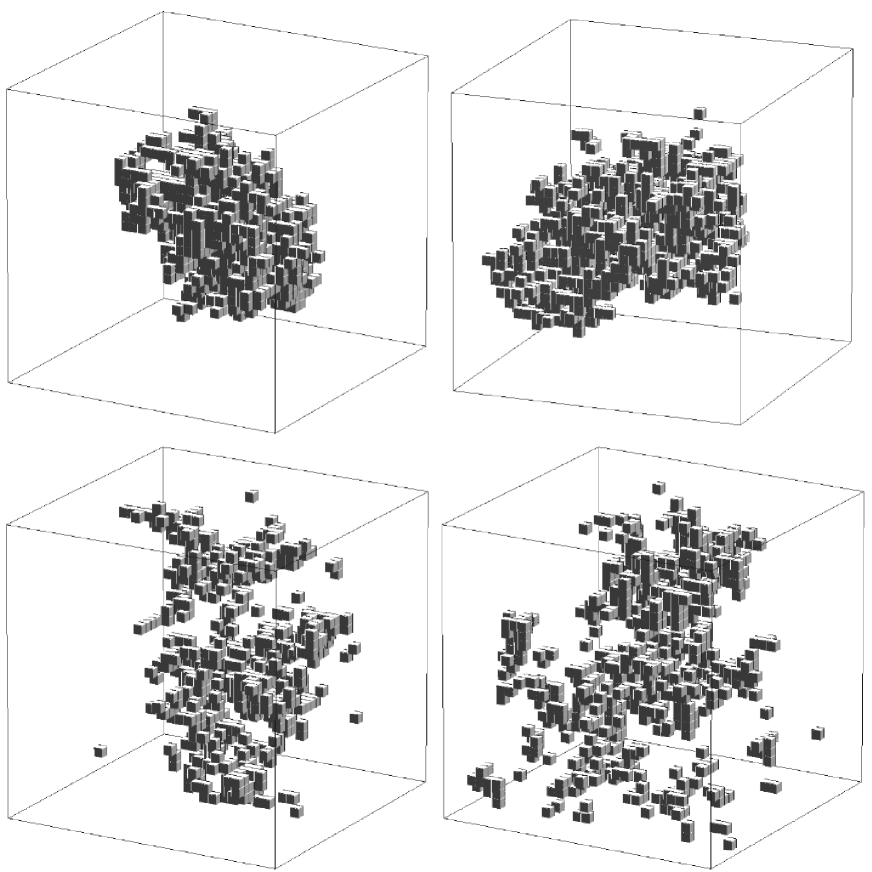
FIG. 8.: Snapshots of four arbritrary chosen avalanche clusters for $D=3$ (upper left), $D=4$ (upper right), and $D=5$ (lower left and right). For $D\geq 4$ three dimensional cuts through the center of mass are shown. In the three dimensional avalanche a loop can be seen in the upper left part of the avalanche cluster.

   

Our results are in contrast to previous investigations performed by Jánosi and Czirók [22]. They calculated the number of toppled site $N(r)$ inside a sphere with radius $r$. The sphere is centered at the center of mass of the avalanche cluster. The fractal dimension $D_{f}$ is obtained from the scaling law $N(r)\sim r^{D_{f}}$. Considering one system size ($L=100$ in $D=3$) they found that the fractal dimension is given by $D_{f}\approx 2.75$, i.e., the avalanches already display a fractal behavior in three dimensions. We performed the same analysis and reproduced their results within the error-bars. Analyzing various system sizes, however, we find that the apparent fractal dimension depends on the system size and tends to $D_{f}=3$ with increasing $L$ (not shown) in agreement with our results, discussed above.

V discussion

TABLE I.: Values of the exponents of the BTW model in various dimensions.

	$D=2$	$D=3$	$D=4$	$D=5$	$D=6$
$\tau_{s}$	1.293	$\tau_{d}$	$\tau_{d}$	$\tau_{d}$	$\tau_{d}$
$\tau_{d}$	$\frac{4}{3}$	$\frac{4}{3}$	$\frac{3}{2}$	$\frac{3}{2}$	$\frac{3}{2}$
$\tau_{t}$	$\frac{3}{2}$	$\frac{8}{5}$	$2$	$2$	$2$
$\tau_{r}$	$\frac{5}{3}$	$2$
$z$	$\frac{4}{3}$	$\frac{5}{3}$	$2$	$2$	$2$
$\gamma_{dr}$	$2$	$3$	$4$	$4$	$4$

In the following we examine the avalanche exponents as a function of the dimension $D$. Consider the average avalanche size

$$\langle s\rangle_{L}\;=\;\int s\,P_{s}(s,L)\,\mbox{d}s.$$ (14)

Using the finite size scaling ansatz [Eq. (11)] which works for $D\geq 3$ one gets [23]

$$\langle s\rangle_{L}\;\sim\;L^{2\nu_{s}-\beta_{s}}\;=\;L^{\gamma_{sr}(2-\tau_{s})},$$ (15)

if $\tau_{s}<2$. On the other hand it is known exactly [4] that $\langle s\rangle_{L}\sim L^{2}$ in $D=2$ and arguing that in undirected models particles diffuses out to the boundary one gets the same result independent of the dimension [23]. Like Grassberger and Manna [14] we plot in Fig. 9 the average avalanches size as a function of the system size for various dimensions. Except of deviations for small system sizes all data points collapse on a single curve. Thus one concludes that the equation $2=\gamma_{sr}(2-\tau_{s})$ is fulfilled. Neglecting multiple toppling ($\tau_{s}=\tau_{d}$ and $\gamma_{sr}=\gamma_{dr}$) which is valid for $D\geq 3$ and using that the avalanches are not fractal ($\gamma_{dr}=D$) which is fulfilled for $D\leq D_{u}$ one gets

$$\tau_{d}\;=\;2\,-\,\frac{2}{D},$$ (16)

for $3\leq D\leq D_{u}$ [24]. This equation was already derived in the continuum limit by Zhang using energy conservation and the local nature of energy transfer [19]. Now we see that the failure of this equation for $D=2$ is caused by multiple toppling events which are essential in the two dimensional model only. For $D\geq 3$ multiple toppling can be neglected and Eq. (16) is fulfilled. Using

$$z\,(\tau_{t}-1)\;=\;\gamma_{dr}\,(\tau_{d}-1)$$ (17)

and Eq. (10) the duration exponent $\tau_{t}$ is given by

$$\tau_{t}\;=\;4\,\frac{D-1}{D+2},$$ (18)

again for $3\leq D\leq D_{u}$.

FIG. 9.: The average avalanche size $\langle s\rangle_{L}$ as a function of the system size in various dimensions. The solid line corresponds to the power-law $\langle s\rangle_{L}\sim L^{2}$ which is exactly in $D=2$ [4].

TABLE II.: Values of the exponents of $D$-state model in various dimensions.

	$D=2$	$D=3$	$D=4$	$D=5$
$\tau_{s}$	$\frac{14}{11}$	$\approx\frac{14}{10}$	$\tau_{d}$	$\tau_{d}$
$\tau_{d}$	$\frac{11}{8}$	$\approx\frac{13}{9}$	$\frac{3}{2}$	$\frac{3}{2}$
$\tau_{t}$	$\frac{3}{2}$	$\approx\frac{37}{21}$	$2$	$2$
$\tau_{r}$	$\frac{7}{4}$	$\approx\frac{7}{3}$
$z$	$\frac{3}{2}$	$\approx\frac{7}{4}$	$2$	$2$
$\gamma_{dr}$	$2$	$\approx 3$	$4$	$4$

Finally we briefly report results of similar investigations of the related $D$-state sandpile model based on Manna’s two-dimensional two-state model [18]. Here the critical height $h_{c}$ equals the dimension $D$ and an unstable site relaxes to zero, whereby the particles are distributed randomly among the nearest neighbors. Again we find that the upper critical dimension is $D_{u}=4$. In contrast to the BTW model the dimensional dependence of the dynamical exponent is given by $z=(D+4)/4$. Our preliminary results for $D=3$ are $\tau_{s}\approx\frac{14}{10}$, $\tau_{d}\approx\frac{13}{9}$, $\tau_{t}\approx\frac{37}{21}$, $\tau_{r}\approx\frac{7}{3}$, and $\gamma_{dr}\approx 3$. We find that $\tau_{d}$ is definitely larger than $\tau_{s}$ (in agreement with [17]), i.e., multiple toppling events are relevant in the three dimensional model. Because in the $D$-state model the toppling processes are isotropic on average only holes inside an avalanche cluster can occur. But nevertheless, we find that $\gamma_{dr}=D$ for $D\leq D_{u}$, i.e., these holes occur only on finite sizes and do not contribute to the scaling behavior. Above the critical dimension $D_{u}=4$ the avalanches have fractal dimension 4. In $D=4$ and $D=5$ the model is characterized by the mean field exponents, comparable to the BTW model. The values of the exponents are listed in Table II.

VI Conclusions

We studied numerically the dynamical properties of the BTW model on a square lattice in various dimensions. Using a finite size scaling analysis we determined the probability distribution exponents, the dynamical exponent, and the dimension of the avalanches. Our analysis reveals that multiple toppling events are relevant in the low dimensional case only and can be neglect for $D\geq 3$. For $D=3$ the exponents are given by $\tau_{r}=2$, $\tau_{t}=\frac{8}{5}$, $\tau_{d}=\frac{4}{3}$, and $z=\frac{5}{3}$. For $D\geq 4$ the exponents agree with the mean field and Bethe lattice exponents, respectively. We conclude from our numerical results that below the critical dimension the dynamical exponent $z$ is given by $z=(D+2)/3$. The avalanche clusters are simply connected for $D=2$ only. For $D>2$ loops occur but do not contribute to the scaling behavior until the embedding dimension exceeds the upper critical dimension $D_{u}$. Above $D_{u}$ the avalanches are fractal with the fractal dimension $4$.