Transport of Surface States in the Bulk Quantum Hall Effect

Abstract

The two-dimensional surface of a coupled multilayer integer quantum Hall system consists of an anisotropic chiral metal. This unusual metal is characterized by ballistic motion transverse and diffusive motion parallel ($\hat{z}$) to the magnetic field. Employing a network model, we calculate numerically the phase coherent two-terminal z-axis conductance and its mesoscopic fluctuations. Quasi-1d localization effects are evident in the limit of many layers. We consider the role of inelastic de-phasing effects in modifying the transport of the chiral surface sheath, discussing their importance in the recent experiments of Druist et al.[1]

I Introduction

In a two-dimensional incompressible quantized Hall state, the low energy excitations are confined to the edge of the sample. These edge states provide a simple way to understand transport in both integer and fractional quantum Hall systems.[2] For the integer quantum Hall effect with one filled Landau level, there is a single edge mode, describable in terms of a free chiral Fermion. Edge states in the FQHE are believed to be (chiral) Luttinger liquids, and have been probed via tunneling spectroscopy in several recent experiments.[3]

In recent years there has been much interest in multi-layer quantum Hall systems. In double layer systems the layer index plays the role of a pseudo-spin, and these systems have revealed a number of new surprises. In the opposite extreme with many layers, the samples become three-dimensional, and a number of new features are expected. In such bulk samples with interlayer tunneling smaller than the Landau level spacing, the (integer) quantized Hall effect in each layer should survive, and the sample exhibit a 3d quantum Hall phase. Chalker and Dohmen[4] have recently discussed the phase diagram in such a system, in a model of non-interacting electrons with disorder. In the absence of disorder, the Landau levels will be broadened into bands in the presence of interlayer tunneling, $t$. Disorder further broadens these bands. Near the band centers a diffusing 3d metallic state is expected. In the tails of the Landau bands, the bulk states are localized, but current carrying edge states nevertheless lead to a quantum Hall effect. For one full Landau level, each layer has a single chiral free Fermion edge state, which together comprise a 2d sub-system - a chiral surface sheath.[4, 5] This surface phase forms a novel 2d chiral metal system, which has been analyzed theoretically by a number of authors. [6, 7, 8, 9, 10, 11] In the presence of impurity scattering, the transport is predicted to be very anisotropic, with ballistic in-plane motion and diffusive motion parallel to the magnetic field. Vertical transport in such a multilayer sample was first investigated experimentally in Ref. [12], and has recently been revisited by Druist et al.[1]  The latter experiment provides striking evidence of the novel behavior characteristic of the chiral metal.

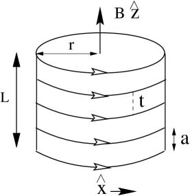
FIG. 1.: Geometry of a multilayer quantum Hall system with an interlayer hopping amplitude $t$ allowing vertical transport. With $N$ layers the system has height $L=Na$, and a circumference $C=2\pi r$.

Most of the theoretical work on the chiral metal phase has focused on the mesoscopic regime, with the sample assumed smaller than the phase breaking lengths. The predicted behavior for such phase coherent transport is very rich, with three different possible regimes (see Fig. 2) connected by universal crossovers.[5, 6, 7, 9]

The purpose of this paper is two-fold. First, we revisit the phase coherent regime and study in detail the conductance and its fluctuations. Performing numerical transfer matrix calculations on a directed network model for the chiral metal enables us to extract the conductance and its fluctuations in the various regimes, and compare directly with earlier analytic approaches. We then address the important role of phase breaking processes, which have been ignored in earlier theoretical discussions.

The paper is organized as follows. In Section II we briefly review the existing theoretical predictions for the phase coherent transport. In Section III we describe the network model, and extract numerically the phase coherent conductance in the various regimes. Section IV is devoted to a discussion of de-phasing processes, and Section V to prospects and conclusions.

II Phase Coherent Regime

For one full Landau level, there is a single free chiral Fermion edge mode in each layer, as depicted in Fig. 1. In the presence of an interlayer tunneling amplitude, $t$ (assumed much smaller than $\hbar\omega_{c}$), these chiral edge modes disperse along the z-axis, and form one-half of an open 2d Fermi surface. Impurities causes electrons to scatter about the Fermi surface, as in any dirty metal. Due to the chiral nature, the in-plane motion remains ballistic with velocity $v$, even in the presence of impurities. However, the (inter-layer) motion parallel to the field becomes diffusive, with diffusion constant $D$. Easier to measure than the ballistic velocity or diffusion constant is the z-axis (2d sheet) conductivity, $\sigma_{zz}$, related to $v$ and $D$ via an Einstein relation:[5]

$$\sigma_{zz}=e^{2}\rho D={D\over va}\cdot{e^{2}\over h}$$ (1)

where $a$ is the inter-layer (lattice) spacing and $\rho=1/hva$ the density of states. It will be convenient to introduce a dimensionless z-axis conductivity via $\sigma_{zz}=(e^{2}/h)\sigma$.

For a mesoscopic sample with finite circumference, $C$, and number of layers, $N=L/a$, there are several important time scales. For ballistic motion with velocity $v$, an electron circumnavigates the sample in a time $\tau_{c}=C/v$. In a time $\tau_{L}=L^{2}/D$ an electron will diffuse from the bottom to the top of the sample. The transport will be phase coherent provided the de-phasing time, $\tau_{\phi}$, is much longer than both $\tau_{c}$ and $\tau_{L}$. In principle, this mesoscopic regime exists for any sample at sufficiently low temperatures, since the de-phasing time diverges as $T\rightarrow 0$ ($\tau_{\phi}\sim\hbar/k_{\rm B}T$ in the quasi-1d limit of interest). Here we focus on the fully coherent regime, returning to de-phasing effects in Section V.

For a sample with finite circumference, $C$, there are two important length scales along the z-axis, which demarcate the boundaries between three regimes (see Fig. 2). [5, 6, 9] Upon circumnavigating the sample once, an electron will diffuse along the z-axis a distance $L_{0}=\sqrt{D\tau_{c}}$, which can be expressed in terms of the measurable z-axis conductivity, $\sigma$, as,

$$L_{0}=(a\sigma C)^{1/2}.$$ (2)

For finite $C$ with $L\rightarrow\infty$ the system is one-dimensional, and localization along the z-axis is expected. The (typical) localization length, $\xi$, for such a quasi-1d system is proportional to the (dimensionless) 1d conductivity, $\xi\sim\sigma_{1d}$, which can be written,

$$\xi=2\sigma C.$$ (3)

Thus both $L_{0}$ and $\xi$ depend only on geometrical parameters, and the measurable z-axis conductivity, $\sigma$. Notice that $(\xi/a)=2(L_{0}/a)^{2}$, so that provided $L_{0}\gg a$ one has $\xi\gg L_{0}$.

As the height $L$ of the sample varies, three regimes are possible (see Fig. 2). For $L<L_{0}\ll\xi$, an electron typically diffuses from the bottom to the top of the sample before circumnavigating the sample once. In this 2d chiral metal regime, an electron suffers de-phasing in the leads before circling the sample. For $L_{0}\ll L\ll\xi$, the electron circles the sample many times, and phase coherent processes around the sample are important. The system behaves like a phase coherent quasi-1d metal. Finally, for $L\gg\xi$ 1d localization effects dominate, and the system is a 1d (localized) insulator.

FIG. 2.: Three different regimes of the phase coherent transport of the surface sheath of a sample with height $L$ and circumference $C$. Both $L_{0}$, the typical distance an electron diffuses along the z-axis upon circling the sample once, and $\xi$, the 1d localization length, can be deduced from the measurable z-axis conductivity and geometrical parameters, as discussed in the text.

The predicted behavior for the phase coherent z-axis conductance and it’s mesoscopic fluctuations depends sensitively on which regime the system is in. Consider first the (dimensionless) mean two-terminal conductance along the z-axis, $\overline{G}$, where the overbar denotes an average over disorder realizations. In both the 2d chiral metal and the 1d metal regimes, ohmic behavior is predicted with[9],

$$\overline{G}={C\over L}\sigma+O(L/\xi).$$ (4)

The usual “weak localization” corrections which are of order $(L/\xi)^{0}$ are absent due to the breaking of time reversal invariance. In the 1d insulating regime strong localization is operative, and the mean conductance is predicted to fall off exponentially with a universal form (for $L\gg\xi$),[13]

$$\overline{G}=2(\pi\xi/2L)^{3\over 2}\exp(-L/2\xi).$$ (5)

Conductance fluctuations are also of interest, which can be characterized by the variance, $\overline{\delta G^{2}}$, where $\delta G=G-\overline{G}$. In the 2d chiral metal and 1d metal regimes, Gruzberg et al.[11] have shown that the variance can be written,

$$\overline{\delta G^{2}}=\Phi(L/L_{0})+O(L/\xi),$$ (6)

where $\Phi(X)$ is a universal scaling function which smoothly connects the two regimes. Deep within the 1d metal regime the variance approaches a universal number well known for quasi-1d metals: $\Phi(L/L_{0}\rightarrow\infty)=1/15$. In the 2d chiral metal regime, $\Phi(L/L_{0})\sim(L_{0}/L)^{2}$ for $L/L_{0}$ small. The conductance fluctuations are large in this limit, since the sample effectively breaks up into $\tau_{c}/\tau_{L}=(L_{0}/L)^{2}$ incoherent regions which add independently to the conductance and it’s fluctuations. Gruzberg et al.[11] have obtained the full universal scaling function, $\Phi(X)$, which interpolates between these two limits. In the 1d localized regime, the conductance is expected to be very broadly distributed, with an approximate log-normal distribution.

III Numerics

A Network model

Following Chalker and Dohmen,[4] we employ a simple network model to study phase coherent transport of the surface sheath. The network model consists of directed links carrying electron current, connected via node parameters, as depicted in Fig. 3. All links carry current in the $x-$direction, as appropriate for the chiral surface sheath. Scattering at the nodes is characterized by a (real and dimensionless) transmission amplitude, $t_{0}$, for tunneling in the $z-$direction between edge states in neighboring layers. For a given node the $S-$ matrix relating incoming to outgoing amplitudes is given explicitly by,

$$\left(\begin{array}[]{c}w_{\rm out}\\ v_{\rm out}\end{array}\right)=\left(\begin{array}[]{cc}r_{0}&t_{0}\\ t_{0}&-r_{0}\end{array}\right)\left(\begin{array}[]{c}w_{\rm in}\\ v_{\rm in}\end{array}\right),$$ (7)

with $t_{0}^{2}+r_{0}^{2}=1$. By construction, this matrix conserves the current, $|w_{\rm in}|^{2}+|v_{\rm in}|^{2}=|w_{\rm out}|^{2}+|v_{\rm out}|^{2}$. To model the disorder, the electrons are assumed to acquire a random phase along each link connecting adjacent nodes, taken for simplicity to be independent and uniformly distributed on the interval $[0,2\pi]$.

Periodic boundary conditions are taken in the ballistic $x-$direction, with the circumference $C=2bN_{c}$, where $b$ is the length of a single link in the $x-$direction and $N_{c}$ is the total number of inter-layer tunneling nodes connecting adjacent edge modes (see Fig. 3). The network consists of $N$ edge modes, with spacing $a$ and a total “height” of $L=Na$.

The conductance along the $z-$axis is obtained by computing the transmission of electrons from the bottom to the top of the sample. Specifically, we use the two-terminal Landauer formula to relate the (dimensionless) conductance $G$ to the transmission matrix t:[14]

$$G={\rm tr}[{\bf t}^{+}{\bf t}].$$ (8)

The matrix elements, $t_{ij}$, are the amplitudes for an electron incident into channel (or node) $i$ on the bottom edge to be transmitted into channel $j$ on the top edge. Here $N_{c}$ is the number of channels.

The transmission matrix is computed numerically by iterating a transfer matrix from the bottom to the top of the sample. This involves re-expressing each node in a form relating the amplitudes in one edge mode to the amplitudes in the adjacent edge mode:

$$\left(\begin{array}[]{c}w_{\rm in}\\ w_{\rm out}\end{array}\right)=\left(\begin{array}[]{cc}r_{0}/t_{0}&1/t_{0}\\ 1/t_{0}&r_{0}/t_{0}\end{array}\right)\left(\begin{array}[]{c}v_{\rm in}\\ v_{\rm out}\end{array}\right).$$ (9)

We study a range of system sizes with the channel number $N_{c}=4,8,16,32$ and the layer number $N=8,10,12,16$. Being interested in conductance fluctuations, it is necessary to evaluate the conductance exactly for each given disorder realization. The self averaging Lyapunov exponents for a sample with $L\rightarrow\infty$ cannot be used to extract the sample to sample fluctuations in a finite system. This restriction imposes rather serious constraints on the accessible system sizes.

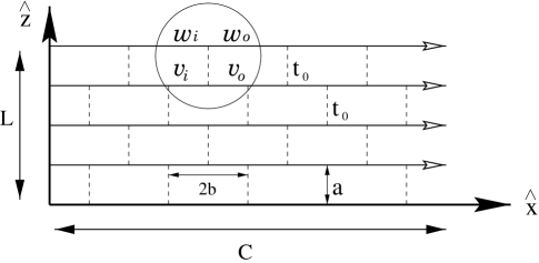
FIG. 3.: Network model for the surface sheath. Here $N=L/a=4$ chiral edge modes are interconnected with dimensionless tunneling $t_{0}$, with periodic boundary conditions taken in the $\hat{x}$ direction of circumference $C$. The $z-$axis conductance is computed by employing a transfer matrix acting in the $z-$direction.

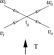
FIG. 4.: The single node inside the circle in Fig. 3 (re-drawn in a more conventional way) represented by the matrix in Eqn. (3.3). The transfer matrix progresses from bottom to top.

Since the microscopic parameters of the network model, $t_{0}$ and $b$, are not experimentally meaningful quantities, it is useful to relate them to a macroscopic observable, namely the measurable $z-$axis sheet conductivity of the surface sheath, $\sigma$. As shown by Chalker and Dohmen,[4] this is possible for the network model, by summing the Feynman paths analytically. Specifically, consider paths that connect the incident electrons on the bottom edge to the transmitted electrons on the top edge. For $C\rightarrow\infty$ these paths do not fully circumnavigate the sample so that the interference between paths wrapping around the sample a different number of times - possible for finite $C$ - is completely absent. In the absence of such interference the ensemble averaged conductance reduces to a sum of classical probabilities: Any two paths which pass through a different sequence of directed links will have a random relative phase, so that the interference term will vanish upon ensemble averaging. To sum the classical probabilities of these non-winding paths we follow Chalker and Dohmen,[4] and consider the transmission probability for an electron incident in one channel (say $i$) to be transmitted through $N$ layers: $T_{N}=\sum_{j}|t_{ij}|^{2}$. One can then express $T_{N+1}$ in terms of $T_{N}$ and the single layer transmission probability, $T_{1}=t_{0}^{2}$, as a geometric sum:

$$T_{N+1}=\sum_{n=0}^{\infty}T_{N}(R_{1}R_{N})^{n}T_{1},$$ (10)

where $R_{N}=1-T_{N}$ is the reflection probability off $N$ layers. Carrying out this geometric sum, gives the recursion relation,

$${1\over T_{N+1}}={1-T_{1}\over T_{1}}+{1\over T_{N}},$$ (11)

which can be readily solved for $T_{N}$. The average conductance in the absence of interference between paths winding around the sample is simply $\overline{G}_{0}=N_{c}T_{N}$, with $N_{c}$ the number of channels. It is given exactly by,

$$\overline{G}_{0}={N_{c}\over N}{t_{0}^{2}\over 1-t_{0}^{2}(1-1/N)},$$ (12)

as obtained by Chalker and Dohmen[4] for $1/N\rightarrow\infty$. The $z-$axis sheet conductivity follow from Ohms law, $\sigma=L\overline{G}_{0}/C$, which in the limit $C,L\rightarrow\infty$ becomes,

$$\sigma={a\over 2b}{t_{0}^{2}\over 1-t_{0}^{2}}.$$ (13)

Having related the conductivity to the network parameters, the mesoscopic crossover lengths $L_{0}$ and $\xi$ for a finite size network model can be readily obtained from Eqn. (2) and (3).

The exact result for the conductance Eqn. (12) in the absence of interference between winding paths should be valid even for finite circumference, provided $C$ is large enough so that winding paths are rare. The condition for the validity of ignoring the interference between winding paths is that $L\ll\sigma C\sim\xi$, so that the sample is in the 2d chiral metal or 1d metal regimes.

Notice that $\overline{G}_{0}$ in Eqn. (12) is well defined even as $t_{0}\rightarrow 1$. In this limit, the motion along the z-axis also becomes ballistic (for finite $N$), and each channel is perfectly transmitted with $\overline{G}_{0}\rightarrow N_{c}$. It will be convenient to define an Ohmic conductance,

$$G_{ohm}\equiv C\sigma/L=\xi/2L,$$ (14)

which coincides with $\overline{G}_{0}$ when $L$ is large enough that the $z-$axis motion is diffusive. As defined, $G_{ohm}$ diverges with $\sigma$ as $t_{0}\rightarrow 1$. The crossover from diffusive to ballistic $z-$axis motion occurs when $G_{ohm}\approx N_{c}$.

The 2d chiral metal regime requires that $L\ll L_{0}$, or equivalently $N\ll G_{ohm}$. However, to avoid a crossover into the ballistic regime of the network model requires $G_{ohm}<N_{c}$. Thus 2d chiral metal behavior is expected for $N\ll N_{c}$. Since this limit is difficult to access numerically, we focus below primarily on the 1d metallic and localized regimes.

B Results

In Fig. 5 we show results for the ensemble-averaged two-terminal conductance, $\overline{G}$, computed numerically from the network model, plotted versus the tunneling parameter $t_{0}^{2}$ for various different channel numbers, $N_{c}$, at fixed height, $N=12$. The solid lines are the “classical” conductance, $\overline{G}_{0}$ Eqn. (12), valid in the absence of interference between winding paths, and the dashed lines the “Ohmic conductance”, $G_{ohm}=C\sigma/L$. Notice that $\overline{G}_{0}$ gives a good fit to the numerical data, except in the low conductance regime, $\overline{G}<1$, where 1d localization effects are expected. The deviations from the classical behavior in this regime can be seen more easily in Fig. 6, where we plot the same data for the conductance, but now normalized by $\overline{G}_{0}$. Strong deviations are seen for small $t_{0}^{2}$, where the system enters into the 1d localized regime and interference between winding paths is critical.

FIG. 5.: The mean $z-$axis conductance $\overline{G}$ with fixed height $N=12$ for several different circumferences, plotted versus the dimensionless interlayer tunneling probability $t_{0}^{2}$. The solid lines are $\overline{G_{0}}$ given by Eqn. (3.6), and the dashed lines are the Ohmic conductances $G_{ohm}=\xi/2L$ given in Eqn.’s (3.7) and (3.8).

FIG. 6.: The mean conductance $\overline{G}$ from Fig. 5 replotted after normalizing by $G_{0}$. The ratio $\overline{G}/G_{0}$ deviates from one as the system becomes localized.

In order to study the crossover from the 1d metallic to localized regime, we plot in Fig. 7 the mean conductance for $N=12$, normalized by $G_{ohm}=2\xi/L$, versus $2L/\xi$. The data shows a crossover from a 1d metallic regime with Ohmic behavior, $\overline{G}\approx G_{ohm}$, to a 1d localized regime where the conductance vanishes exponentially for $L\gg\xi$. The solid line is the prediction from Mirlin et al.,[13] for the mean conductance of a quasi-1d metallic wire obtained using supersymmetry methods. The agreement is reasonable, but our numerics deviate from the universal form of Mirlin et al.[13] both at large and small $L/\xi$. The deviations at large $L/\xi$ are presumably due to lattice cutoff effects, since in this regime the localization length along the $z-$axis is comparable to the network model lattice spacing $a$. The deviations for small $L/\xi$ are probably due to finite size effects. Indeed, as the channel number $N_{c}$ increases, the agreement improves. Notice that $\overline{G}/G_{ohm}$ vanishes as $L/\xi\rightarrow 0$ (rather than approaching unity) due to ballistic behavior in the network model: In this limit $t_{0}\rightarrow 1$ and $G_{ohm}$ diverges whereas $\overline{G}$ saturates at the (finite) channel number $N_{c}$.

FIG. 7.: The mean conductance normalized by $G_{ohm}=\xi/2L$ versus $2L/\xi$. For each sample size the points correspond to different values of the hopping probability $t_{0}^{2}$. The solid line is the mean conductance computed analytically for a quasi-1d system taken from Mirlin et al.’s paper.

In addition to the mean conductance, we have computed the sample-to-sample conductance fluctuations. In Fig. 8 we have plotted $\overline{\delta G^{2}}$ versus $2L/\xi$, for height $N=16$ and various different channel numbers. The solid curve is the universal prediction for the variance of the conductance of a quasi-1d wire, obtained by Mirlin et al..[13] This curve shows the crossover from the 1d metallic regime at small $L/\xi$, where the variance approaches the well known universal value, $\overline{\delta G^{2}}=1/15$, to the 1d localized regime where the fluctuations vanish exponentially for $L\gg\xi$. The agreement between our numerical data and the Mirlin et al.[13] theory is quite striking. Again, the deviations for $L/\xi\rightarrow 0$ are due to the ballistic regime in the network model for $t_{0}\rightarrow 1$ (with finite $N$), where the conductance fluctuations vanish. For $L\gg\xi$ the localization length approaches the lattice spacing. The numerics and theory agree very well near the peak in the crossover regime.

FIG. 8.: Variance of the conductance for different sample sizes and hopping amplitudes $t_{0}^{2}$, all plotted versus $2L/\xi$. The solid line is the variance of the conductance for a quasi-1d sample, computed analytically by Mirlin et al..

Finally, we mention briefly our effort to extract numerically the conductance in the 2d chiral metal regime. This regime requires that $L\ll L_{0}$, or equivalently $N\ll G_{ohm}$. However, to avoid the ballistic regime when $t_{0}\rightarrow 1$, we must require that $G_{ohm}<N_{c}$, so that we need $N\ll N_{c}$. We have focussed on the conductance fluctuations in this regime, since these are predicted to behave very differently than in the 1d metal, diverging with $L/L_{0}\rightarrow 0$ as $\overline{\delta G^{2}}\sim(L_{0}/L)^{2}$. In Fig. 9 the variance of the conductance is shown for “short” and “wide” samples, with height $N=8$ and width $N_{c}=16,32,64$, plotted versus $L/L_{0}$ where $L_{0}=\sqrt{a\sigma C}$. For each width, $N_{c}$, we have varied the tunneling probability, $t_{0}^{2}$, to get the set of data points. The solid line is the analytic prediction from Gruzberg et al., [11] for the conductance variance in the crossover regime between the 1d and 2d chiral metal. Unfortunately, the agreement with the analytic result is quite poor, although the agreement improves for the widest sample with $N_{c}=64$. Indeed, the large enhancement in the variance for the sample with $N_{c}=64$ in the range $1<L/L_{0}<3$ is consistent with the theoretical expectations. The sharp drop in the conductance fluctuations for smaller $L/L_{0}$ is due to the crossover from diffusive to ballistic motion in the network model. The local maxima for $N_{c}=16$ at $L/L_{0}\approx 4$ is the same maxima as in Fig. 8, and indicates a crossover into the 1d localized regime for larger $L/L_{0}$, where the Gruzberg et al. results do not apply.

FIG. 9.: Variance of the conductance versus $L/L_{0}$ for three different “short” and “wide” samples at various values of $t_{0}^{2}$. The solid line is the conductance variance computed analytically by Gruzberg et al. in the universal crossover regime between the 1d and 2d chiral metals. The dashed line is at $\overline{\delta G^{2}}=1/15$ - the value in the 1d metal regime.

IV Inelastic Effects

The above results for the phase coherent transport are dramatically modified in the presence of phase breaking effects. De-phasing effects can be characterized by a phase breaking time, denoted $\tau_{\phi}$, which is the time an electron can propagate before having its phase randomized by interactions with other electrons or phonons. In the extreme anisotropic limit of the surface sheath with vanishing interlayer tunneling, $t=0$, an electron propagating in one edge state will interact via Coulomb forces with electrons in neighboring edges states, and can suffer phase breaking inelastic scattering events. Being in 1d, the scattering rate, evaluated to leading order in the interactions strength $u$, is linear in temperature: $1/\tau_{\phi}=c(ul_{B}/2\pi\hbar v)^{2}k_{B}T/\hbar$, with $c$ an order one constant, $l_{B}$ the magnetic length and $v$ the edge velocity. In practice, the dimensionless ratio $ul_{B}/\hbar v$ is itself also of order one, so that $1/\tau_{\phi}\sim k_{B}T/\hbar$. For non-zero but small interlayer tunneling, the de-phasing rate will probably crossover to a two-dimensional $T^{2}$ dependence at very low temperatures.

Associated with the de-phasing time are two de-phasing lengths: (i) $l_{\phi}=v\tau_{\phi}$, the distance an electron propagates in the ballistic $x-$direction before de-phasing and (ii) $L_{\phi}=\sqrt{D\tau_{\phi}}=\sqrt{\sigma al_{\phi}}$ the distance an electron diffuses parallel to the field in time $\tau_{\phi}$. Consider the transport geometry in Fig. 1, in which metallic contacts are applied at $z=0$ and $z=L$. For $L_{\phi}\gg L$, an electron diffuses between the two contacts before being de-phased. In this case, transport is mesoscopic, and the above phase-coherent results apply.

For $L_{\phi}\ll L$, however, inelastic scattering occurs within the sample, and we must reconsider transport properties. There are two such important incoherent regimes, depending upon the relative magnitude of $l_{\phi}$ and $C$. For $l_{\phi}\ll C$, the electron does not fully circumnavigate the sample before suffering a phase breaking collision. In this situation, electron paths which wind a different number of times around the sample do not interfere. As a result the system cannot explore the three phase coherent regimes discussed in Sections II and III. Instead, the system is appropriately described as a phase incoherent 2d chiral metal. Nevertheless, there are (small) mesoscopic fluctuations expected even in this limit, which we discuss below. In the opposite extreme of $\l_{\phi}\gg C$, the electron can propagate many times around the sample before phase breaking. In this case, the one-dimensional motion parallel to the field is phase coherent up to a length scale $L_{\phi}$. The system should behave like an incoherent quasi-1d wire, with $L_{\phi}$ the appropriate (1d) de-phasing length, as we discuss further below.

To describe the transport behavior in these incoherent regimes, we employ arguments first applied in Ref. [15]. The important observation is that the sample can be subdivided into “patches”, whose size is the maximum area over which an electron diffuses in time $\tau_{\phi}$. Each such region effectively acts as a classical resistor, and the whole sample then as a random resistor network, the properties of which are well understood.

First consider $l_{\phi}\ll C$. Then the patches have dimensions $l_{\phi}$ by $L_{\phi}$, and form an array of size $C/l_{\phi}$ by $L/L_{\phi}$. Denoting by $g_{i}$ the (dimensionless) conductance (along the $z-$axis) of the $i^{th}$ patch, Ohm’s law gives an average patch conductance of $\overline{g}_{i}=g_{0}=\sigma l_{\phi}/L_{\phi}$. The conductance fluctuations in each patch, $\delta g_{i}=g_{i}-g_{0}$, are of order one, - being equivalent to the conductance fluctuations of a fully coherent network at the boundary between the 1d and 2d metal regimes. Since the mean conductance can be written $g_{0}=L_{\phi}/a$, provided the patch size is larger than the lattice spacing, $L_{\phi}\gg a$, the conductance fluctuations in each patch are much smaller than the mean conductance: $\delta g_{i}\ll g_{0}$. In this limit, both the total conductance, $\overline{G}$, and it’s variance, $\delta G^{2}=\overline{G^{2}}-(\overline{G})^{2}$, can be easily evaluated. A simple estimate is to imagine connecting the resistors (patches) only vertically (an approximation which gives the correct result for the conductance fluctuations up to an order one prefactor). Then for each column, the patch resistances add, so that $\delta G_{col}^{2}\approx(L_{\phi}/L)^{3}$, which is independent of $g_{0}$. Contributing in parallel, the conductances of the $N_{col}=C/l_{\phi}$ columns add, so that the variance of the total conductance is simply $\delta G^{2}=N_{col}\delta G_{col}^{2}$. This can be written in the form:

$${\delta G^{2}\over\overline{G}^{2}}\approx{a^{2}\over{CL}}\left[{1\over\sigma}{l_{\phi}\over a}\right]^{1/2},$$ (15)

with $\overline{G}=C\sigma/L$. Notice that the conductance fluctuations have an appreciable temperature dependence entering through $l_{\phi}$, growing in magnitude at low temperatures. The mean conductance, however, remains temperature independent.

Consider next the 1d incoherent limit with $l_{\phi}\gg C$, in which the electron propagates many times around the sample before de-phasing. In this limit, the $L/L_{\phi}$ classical patch resistors form a one-dimensional random chain, and have dimensions $C$ by $L_{\phi}$. Due to 1d localization effects, the conductance of each such segment will depend strongly on it’s length, $L_{\phi}$, and hence on the temperature $T$. For example, when $L_{\phi}$ is much smaller than the 1d localization length $\xi$, the (mean) conductance of each segment is given by,

$$G_{seg}(L_{\phi})=(\sigma C/L_{\phi})-{2\over 45}{L_{\phi}\over\xi}+O(L_{\phi}/\xi)^{2},$$ (16)

where the first term is Ohm’s law, and the second term reflects the leading 1d localization corrections within the unitary ensemble. In the opposite limit, $L_{\phi}\gg\xi$, one expects a stronger length (and temperature) dependence, $G_{\rm seg}(L_{\phi})\sim\exp(-L_{\phi}/2\xi)$. The total conductance follows by simply adding the series resistances of each of the $L/L_{\phi}$ segments. In the 1d metallic regime with $L_{\phi}\ll\xi$, this gives,

$$\overline{G}={\sigma C\over L}-{2\over 45}{L_{\phi}\over L}{L_{\phi}\over\xi}+...,$$ (17)

which depends on temperature through $L_{\phi}(T)$.

Experimentally, such conductance fluctuations are usually observed not by looking at different samples, but by varying the applied magnetic field in such a way as to change the phases accumulated by interfering electrons and thereby effectively change the disorder. The conductance fluctuations in this context are characterized not only by their amplitude, discussed above, but also by a characteristic field scale $\delta B_{\phi}$. This scale is defined by the amount the applied field must be changed in order that the conductance of a fixed sample becomes uncorrelated with its previous value. Physically, the conductance fluctuations arise from constructive interference of two paths enclosing an area of the phase-coherent patch size. The total change in phase shift around this loop in units of $2\pi$ is simply the change in magnetic flux through this area divided by the flux quantum $\phi_{0}=hc/e$. The characteristic field $\delta B_{\phi}$, which changes the phase around the loop by $O(\pi)$, is thus simply the field which puts, say, half a flux quantum through this coherent area. Assuming the magnetic field has a non-negligible angle to the surface sheath (which we believe to be the case in the experiments of Druist et al.), this gives

$$\delta B_{\phi}\approx\cases{\phi_{0}/l_{\phi}L_{\phi}&$l_{\phi}\ll C$\cr\phi_{0}/CL_{\phi}&$l_{\phi}\gg C$\cr},$$ (18)

in the two incoherent regimes. Note that since $l_{\phi}$ and $L_{\phi}$ increase as temperature is lowered, the conductance varies very rapidly with field at low temperatures.

V Conclusions

We conclude with a comparison of these theoretical results to the experimental data of Druist et al.[1]. Druist et al. have measured the z-axis transport in a series of multilayer quantum Hall samples. Specifically, the samples consisted of 50 layers of $150\AA$ $GaAs$ layers alternating with $150\AA$ $Al_{0.1}Ga_{0.9}As$ barriers doped at their centers with Silicon. The vertical separation between each of the 50 2d electron gases is $a=300\AA$. A simple Kronig-Penney analysis gives an estimate for the z-axis bandwidth of $t=0.12meV$. When the applied magnetic field was tuned onto an integer quantum Hall plateau, the z-axis conductance - dropping with temperature - was found to saturate below about $200mK$. Since the low temperature z-axis conductance scaled linearly with the circumference (perimeter) of the samples, which ranged from $400\mu m\leq C\leq 7mm$, Druist et. al. argued that the conduction was being dominated by the 2d chiral surface sheath. The resulting sheet conductivity along the z-axis was found to be $\sigma\approx 4\times 10^{-4}$ on the $\nu=1$ plateau, and about a factor of three larger for $\nu=2$.

A theoretical estimate for the z-axis conductivity of the surface sheath at one full Landau level can be obtained from[5]

$$\sigma\approx{al_{0}\over\hbar^{2}v^{2}}t^{2},$$ (19)

where $l_{0}$ is an elastic mean free path for edge scattering and $v$ is the (ballistic) edge velocity. Unfortunately, both $v$ and $l_{0}$ are difficult to estimate reliably, depending on the detailed slope and irregularities of the edge confining potential. However, we expect that in the limit of large magnetic field, $l_{0}\gtrsim l_{B}$, where $l_{B}$ is the magnetic length ($l_{0}$ may grow much longer than $l_{B}$ as the edge is made cleaner). Moreover, we expect $v$ to be bounded above by the edge velocity for a hard-wall confining potential, so that $v\lesssim\omega_{c}l_{B}/2\pi$, with $\omega_{c}$ the cyclotron frequency. Putting in these (rough) bounds, we obtain

$$\sigma\gtrsim{{(2\pi)^{2}t^{2}a}\over{\hbar^{2}\omega_{c}^{2}l_{B}}}.$$ (20)

Using the parameters appropriate for the Druist et al. experiment, this gives $\sigma\gtrsim 6\times 10^{-5}$, about an order of magnitude smaller than the experimental value. Given the uncertainties in $v$ and $l_{0}$, as well as possible shifts in $t$ due to interaction effects, this level of agreement is reasonable.

Taking now the measured value of $\sigma$, we can estimate the two length scales which determine the system behavior in the mesoscopic limit. The samples studied by Druist et al. had a range of circumferences $400\mu m\leq C\leq 7mm$, which correspond to lengths $2\leq L_{0}/a\leq 10$ and $10\leq\xi/a\leq 200$, upon using Eqns. (2)–(3). Since $N=L/a=50$ in these experiments, in the mesoscopic limit these samples should span the quasi-1d metal and 1d localized regimes. At low temperatures, we would therefore expect a strong suppression of the conductivity and significant temperature and circumference dependence, especially in the smaller samples. That such effects are not observed must be attributed to inelastic effects. Indeed, as shown below, estimates for the in-plane de-phasing length $l_{\phi}$ give $l_{\phi}\ll C$ even at the lowest temperatures and for the smallest sample. In this limit, mesoscopic effects are greatly suppressed, and the system is best thought of as an incoherent 2d chiral metal. This accounts naturally for the observed low temperature saturation of the conductivity (it remains to be seen whether the weak residual temperature dependence at low $T$ can be fitted to the expected[5] form $\sigma(T)-\sigma(0)\propto T^{2}$).

We can attempt to estimate the de-phasing length $l_{\phi}$ via

$$l_{\phi}=A\left({{hv}\over{ul_{B}}}\right)^{2}{{hv}\over{k_{\rm B}T}},$$ (21)

however there is considerable uncertainty in the parameters - particularly the edge velocity $v$. As a crude estimate we take $A=1$, a dimensionless interaction strength of unity $ul_{B}/hv=1$ and an edge velocity estimated for a hard-wall confining potential $v=\omega_{c}l_{B}/2\pi$. In the $10$ Tesla field used by Druist et al. in the $\nu=1$ plateau and at the lowest temperatures studied of $T=50mK$ this gives the rough estimate $l_{\phi}\sim 20\mu m$

Fortunately, one can also extract estimates for $l_{\phi}$ directly from the experimentally measured conductance fluctuations. In fact, this can be done in two ways, thereby providing a consistency check. One determination is from the amplitude of the fluctuations. Solving Eqn. (15) gives

$$l_{\phi}\approx\tilde{A}{CN^{3}\over\overline{G}^{3}}(\delta G^{2})^{2}.$$ (22)

Because the fourth power of $\delta G$ appears above and the amplitude $\tilde{A}$ is unknown, there is again considerable uncertainty in $l_{\phi}$. For the Druist et al. experiments, we obtain $l_{\phi}\approx 26\mu m$, consistent with the above theoretical estimate.

A second determination comes from the magnetic field scale of the conductance fluctuations. From the above estimates, we see that $L_{\phi}=\sqrt{\sigma al_{\phi}}\lesssim a$ (using the measured $\sigma=4\times 10^{-4}$). This is close to the “incoherent tunneling” limit, and we expect it is appropriate to replace $L_{\phi}\rightarrow a$ in Eqn. (18), giving

$$l_{\phi}\approx{\phi_{0}\over{a\delta B_{\phi}}}.$$ (23)

For the Druist et. al. experiment, this gives $l_{\phi}\approx 3\mu m$ at $T=100mK$, somewhat smaller than the first estimate. In this case there are also considerable uncertainties due primarily to incomplete knowledge of the degree of interlayer flux penetration. However, all three of the above estimates give $l_{\phi}\ll C$.

In summary, the experiments so far are consistent with the picture of an incoherent 2d chiral metal. Several opportunities exist for further theoretical and experimental study. Samples with smaller circumferences in the range of $10$ to $20\mu m$ would be highly desirable, since the mesoscopic regime would then be accessible below several hundred $mK$. In this limit, the rich and varied crossovers between the three mesoscopic regimes could be accessed experimentally. Theoretically, a more quantitative study of inelastic scattering and de-phasing lengths would be desirable in order to achieve a precise comparison with experiment. Particularly interesting from both points of view is the temperature dependence of $1/\tau_{\phi}$, which we believe should exhibit linear scaling with temperature over a broad range. A field-theoretic treatment of de-phasing effects could be useful in providing the desired tighter link with experiments.

REFERENCES

- [1] D. P. Druist, P. J. Turley, and E. G. Gwinn, submitted to Phys. Rev. Lett. (unpublished).
- [2] For a general discussion of edge state transport see, C.L. Kane and M.P.A. Fisher in “Perspectives in the Quantum Hall Effect”, edited by S. Das Sarma and A. Pinczuk ((Wiley, 1997), and references therein.
- [3] F.P. Milliken, C.P. Umbach, R.A.Webb, Solid State Commun. 97, 309 (1996); A.M. Chang, L.N. Pfeiffer, K.W. West, Phys. Rev. Lett. 77, 2538 (1996); P.J. Turley, D.P. Druist, E.G. Gwinn, K. Maranowski, K. Campmann and A.C. Gossard, to be published (1997).
- [4] J. T. Chalker and A. Dohmen, Phys. Rev. Lett. 75, 4496 (1995).
- [5] L. Balents and M. P. A. Fisher, Phys. Rev. Lett. 76, 2782 (1996).
- [6] H. Mathur, Phys. Rev. Lett. 78, 2429 (1997).
- [7] L. Balents, M. P. A. Fisher, and M. R. Zirnbauer, Nucl. Phys. B483, 601 (1996).
- [8] Y.-K. Yu, cond-mat/9611137 (unpublished).
- [9] I. A. Gruzberg, N. Read, and S. Sachdev, Phys. Rev. B 55, 10593 (1997).
- [10] Y. B. Kim, Phys. Rev. B 53, 16420 (1996).
- [11] I. A. Gruzberg, N. Read, and S. Sachdev, cond-mat/9704032 (unpublished).
- [12] H. L. Stormer et al., Phys. Rev. Lett. 56, 85 (1986).
- [13] A. D. Mirlin, A. Muller-Groeling, and M. R. Zirnbauer, Ann. Phys. 236, 325 (1994).
- [14] D. S. Fisher and P. A. Lee, Phys. Rev. B 23, 6851 (1981).
- [15] A. Miller and E. Abrahams, Phys. Rev. 120, 745 (1960).