Dynamical properties of the pinned Wigner crystal

Abstract

We study various dynamical properties of the weakly pinned Wigner crystal in a high magnetic field. Using a Gaussian variational method we can compute the full frequency and field dependence of the real and imaginary parts of the diagonal and Hall conductivities. The zero temperature Hall resistivity is independent of frequency and remains unaffected by disorder at its classical value. We show that, depending on the inherent length scales of the system, the pinning peak and the threshold electric field exhibit strikingly different magnetic field dependences.

Though the exotic possibility of electron crystallisation was discussed decades ago by Wigner [2], its experimental realization has been a challenge due to difficulties in obtaining sufficiently low density electron systems. However, this problem can be circumvented by subjecting the $2$DEG to large magnetic fields which facilitate crystallisation of even dense electron systems. The quest for the Wigner crystal (WC) in mono [3, 4, 5, 6] and bilayer [7] quantum Hall samples indicated the existence of a quaint insulating state at filling fractions where crystallisation was theoretically expected. These and other detailed studies [8] of the insulating state revealed that the diagonal resistivity $\rho_{xx}$ diverges as the temperature $T\to 0$ and shows activated behaviour at finite $T$ whereas the Hall resistivity $\rho_{xy}$ is temperature independent and has a value close to the classical Hall value.

Although measurements of activated linear and non-linear dc conductivity and the luminescence spectrum of radiative recombination [9] were consistent with interpretations in terms of a pinned WC, the finite value seen for $\rho_{xy}$ was unexpected. This prompted other interpretations of the observed insulating phase [10, 11] and in particular the existence of a new phase, the Hall insulator (HI) [11]. The Hall insulator is defined as a phase where $\lim_{\omega\to 0}{{\sigma_{xy}(\omega)}\over{\omega^{2}}}=~{}\rm{cste}$ which yields $\rho_{xx}\to\infty$ and a finite $\rho_{xy}$ in the limit $T\to 0,\omega\to 0$. This was proved only for non interacting electrons in a random potential (i.e an Anderson insulator in presence of a magnetic field) and qualitative arguments suggested that it holds for interacting systems as well. However none of these arguments take into account the possible local crystalline order which could result in radically different physics as compared to the disordered electron fluid. Indeed periodicity plays an important role in other disordered systems, such as vortex lattices [12].

It is thus of prime importance to investigate in detail the transport properties of a pinned WC. Transport properties are especially important here because of the extreme difficulty of a direct experimental verification of local crystalline order. One of the few theoretical attempts made to predict these properties was that of Ref.[13] where the related problem of charge density waves (CDW) in a magnetic field was studied. The harmonic approximation used, however, did not allow the extraction of the detailed frequency dependence of the conductivities. Later works [14] focussed on the sliding state and the effects of free carriers, or on the effect of strong disorder [15]. A noteworthy point is that none of these calculations consider both a lattice structure and modulation of disorder at scales smaller than the lattice spacing [12]. This feature which is absent in CDW turns out to play a crucial role in the physics of the WC.

In this Letter, we compute for the first time the real and imaginary parts of the frequency dependent conductivities of a weakly pinned WC. We find that even some of the main features derived in Ref.[13] are incorrect. The results we obtain provide a basis for comparison with recent experiments which map out the low frequency behaviour of the conductivity[16, 17].

Our starting point is the WC in a magnetic field $B$ with lattice spacing $a$ modelled by an elastic hamiltonian [13]. The electrons at site $i$ are displaced from their mean equilibrium positions ${\bf R}_{i}$ by ${\bf u}({\bf R}_{i},t)$. We also take into account the Coulomb repulsion between density fluctuations. We use the following decomposition ${\bf u}({\bf q})=\hat{\bf q}u_{L}({\bf q})+{\hat{\bf q}}\wedge{\hat{\bf z}}u_{T}({\bf q})$ where $L,T$ denote the longitudinal and transverse components. The corresponding action in the imaginary time formalism is

$$S[u] = \int_{\bf q}\sum_{n}[u^{L}_{q,\omega_{n}}(\rho_{m}\omega_{n}^{2}+cq^{2}+dq)u^{L}_{-q,-\omega_{n}}$$ (1)

$$+ u^{T}_{q,\omega_{n}}(\rho_{m}\omega_{n}^{2}+cq^{2})u^{T}_{-q,-\omega_{n}}+\rho_{m}\omega_{c}\omega_{n}(u^{L}_{q,\omega_{n}}u^{T}_{-q,-\omega_{n}}$$ (2)

$$- u^{L}_{-q,-\omega_{n}}u^{T}_{q,\omega_{n})}]+\int_{\bf x}\int_{0}^{\beta\hbar}d\tau W(x)\rho(x,\tau)$$ (3)

$\rho_{m},\rho_{c}$ are the mass and charge densities. $c$ and $d$ are the shear and bulk modulus respecitvely. For the WC, the presence of Coulomb forces results [14, 18] in a bulk modulus $d={\rho_{c}^{2}\over\epsilon_{0}}$ much greater than the shear modulus $c={{\rho_{c}^{2}a}\over\epsilon_{0}}$ ($\epsilon_{0}$ is the dielectric constant of the substrate). $\omega_{c}={{\rho_{c}B}/{\rho_{m}}}$ is the cyclotron frequency and the Matsubara frequencies at temperature $T$ are $\omega_{n}={{2\pi n}/{\beta\hbar}}$ where $\beta={1/T}$. From (1), we see that the Coulomb interaction affects only the longitudinal modes. The magnetic field couples the transverse and longitudinal modes. $\langle\qquad\rangle$ denote averages over quantum and thermal fluctuations and $\overline{\qquad}$ are disorder averages. For the pure system the quantum fluctuations result in $\langle{\bf u}^{2}\rangle\sim l_{c}^{2}$ where $l_{c}$ is the magnetic length $l_{c}=\sqrt{{\hbar}/{eB}}$. The time-independent disorder potential $W(\bf x)$ is short range correlated (of range $r_{f}$) $\overline{W({\bf x})W({\bf x}^{\prime})}=\Delta\delta_{r_{f}}({\bf x}-{\bf x}^{\prime})$ and couples to the density of electrons $\rho({\bf x},t)=\sum_{i}\delta({\bf x}-{\bf R}_{i}-{\bf u}({\bf R}_{i},t))$. Using the decomposition of the density into lattice harmonics [12] (valid in the absence of topological defects) and replicas to average over disorder we obtain the effective action

$$S_{\text{eff}}= \sum_{a}H[u^{a}]-{1\over{2\hbar}}\int_{\bf x}\int\int d\tau d\tau^{\prime}$$ (5)

$$\sum_{a,b,{\bf K}}\Delta_{K}\cos({\bf K}.({\bf u}^{a}({\bf x}\tau)-{\bf u}^{b}({\bf x},\tau^{\prime})))$$

$a,b$ denote the replica indices, ${\bf K}$ are the reciprocal lattice vectors and $\Delta_{K}\sim\Delta\exp{-{\bf K}^{2}r_{f}^{2}}$. Note that it is important to retain all harmonics. The disorder averaging also yields a term quadratic in the displacements which has been absorbed by a shift in $\bf u$. This shift does not affect the conductivity and we neglect it henceforth. Actions similar to (5) can be used to describe 3-d classical problems such as vortex lattices with correlated disorder [19] and long range interactions.

To study this model we use the gaussian variational method (GVM). This quantitative method allows us to compute the Green functions and hence the conductivity of the system described by (5). Unlike previously used methods [13] the GVM is self-consistent, has no undetermined adjustable parameters and also incorporates important physical feautures of the problem such as the existence of many metastable states. It allows one to go beyond simple static arguments as will be shown later. We introduce the variational action [19]

$$S_{0}={1\over 2}\int_{\bf q}\sum_{n}u_{\alpha,q,\omega_{n}}^{a}G^{{ab}-1}_{\alpha\beta}(q,\omega_{n})u_{\beta,-q,-\omega_{n}}^{b}$$ (6)

where the Green functions $G^{ab}_{\alpha\beta}$ are the variational parameters ( $\alpha,\beta=L,T$ and summations over repeated indices are implicit). They are determined by solving the self-consistent saddle point equations obtained by extremizing the variational free energy $F_{\text{var}}=F_{0}+\langle S_{\text{eff}}-S_{0}\rangle_{0}$. The method extends the one used in [19] and all technical details will be presented in [20]. As in [19] the solution has a replica symmetry broken structure necessary to correctly describe the localization. The final result [20] is a closed set of equations for the connected part of the Green function $G^{-1}_{c\alpha\beta}=\sum_{b}G^{-1}_{\alpha\beta,ab}$ which determine all physical quantities of interest here. These equations are respectively:

$$G_{cT}^{-1} = (cq^{2}+{\rho_{m}}\omega_{n}^{2})+F+{{{\rho_{m}^{2}}\omega_{n}^{2}\omega_{c}^{2}}\over{(cq^{2}+dq+{\rho_{m}}\omega_{n}^{2}+F)}}$$ (7)

$$G_{cL}^{-1} = (cq^{2}+dq+{\rho_{m}}\omega_{n}^{2})+F+{{{\rho_{m}^{2}}\omega_{n}^{2}\omega_{c}^{2}}\over{(cq^{2}+\rho_{m}\omega_{n}^{2}+F)}}$$ (8)

$$G_{cLT}^{-1} = {\rho_{m}\omega_{n}\omega_{c}}+{{(cq^{2}+\rho_{m}\omega_{n}^{2}+F)(cq^{2}+dq+\rho_{m}\omega_{n}^{2}+F)}\over{\rho_{m}\omega_{n}\omega_{c}}}$$ (9)

with $F=I(\omega_{n})+\Sigma(1-\delta_{n,0})$. The localized phase is characterized by a non zero $\Sigma$, from which a length scale $l$ can be defined through $\Sigma=cl^{-2}$. The function $I(\omega_{n})$ is defined as:

$$I(\omega_{n})={2\over\hbar}\int_{0}^{\beta}d\tau(1-\cos(\omega_{n}\tau))(V^{\prime}(\tilde{B}(\tau))-V^{\prime}(B))$$ (10)

where the local diagonal correlation $\tilde{B}(\tau)=1/2\overline{\langle(u(0,\tau)-u(0,0))^{2}\rangle}=1/2({\tilde{B}}_{L}(\tau)+{\tilde{B}}_{T}(\tau))$ and the off diagonal part $B$ are given by:

$${\tilde{B}}_{T,L}(\tau) ={{2\hbar}\over\beta}\int_{q}\sum_{n}G_{cT,L}(1-\cos(\omega_{n}\tau))$$ (11)

$$B ={\hbar\over\beta}\int_{\bf q}[\sum_{n\neq 0}(G_{cL}(q,\omega_{n})+G_{cT}(q,\omega_{n}))]+$$ (13)

$${1\over{cq^{2}+dq+\Sigma}}+{1\over{cq^{2}+\Sigma}}$$

Finally the set of equations close as $\Sigma$ is itself determined by

$$1 = -2V^{\prime\prime}(B)\int_{\bf q}{1\over{(cq^{2}+\Sigma)^{2}}}+{1\over{(cq^{2}+dq+\Sigma)^{2}}}$$ (14)

The primes denote derivatives. All information on the disorder is contained in the auxiliary function $V[B]=(4\hbar)^{-1}\sum_{K}\Delta_{K}\exp(-K^{2}B)$.

In this paper, we focus on the transport properties but other quantities such as positional correlation functions can also be computed [20, 19]. The dynamical conductivities are given by the standard analytical continuation of the Green’s functions $\sigma_{\alpha\beta}(\omega)=i\rho_{c}^{2}\omega G_{\alpha\beta}(q=0,\omega+i\epsilon)$. Rotational invariance combined with fact that a magnetic field breaks parity and time-reversal implies

$$\sigma_{xx} =\sigma_{yy} =\rho_{c}^{2}{{i\omega[-\rho_{m}\omega^{2}+\Sigma+I(\omega)]}\over{(\Sigma-\rho_{m}\omega^{2}+I(\omega))^{2}-\rho_{m}^{2}\omega^{2}\omega_{c}^{2}}}$$ (15)

$$\sigma_{xy} =-\sigma_{yx} =\rho_{c}^{2}{{i\omega[-i\rho_{m}\omega\omega_{c}]}\over{(\Sigma_{1}-\rho_{m}\omega^{2}+I(\omega))^{2}-\rho_{m}^{2}\omega^{2}\omega_{c}^{2}}}$$ (16)

In the absence of disorder one has $I=\Sigma=0$ in (15). $\sigma_{xx}$ vanishes in the dc limit $\omega=0$ and has a $\delta-$function peak at cyclotron frequency $\omega=\omega_{c}$. On the other hand $\sigma_{xy}(\omega=0)={\rho_{c}/B}$ and $\sigma_{xy}$ has a pole at $\omega=\omega_{c}$. In the presence of disorder the crystal is pinned and conductivities develop a new peak at the pinning frequency $\omega=\omega_{p}$. Simultaneously, there is an upward shift of the cyclotron resonance peak from $\omega_{c}$ by a quantity of order $\omega_{p}$.

To obtain the full frequency dependence of the conductivities one needs to compute $I(\omega)$. This can be obtained from the above equations which are valid for all values of $B$. Here we present a solution in the experimentally relevant limit $\omega_{c}\gg{d/c}$. A typical plot of $Re\sigma_{xx}$ obtained by solving (10) numerically is shown in Fig. 1. Since $I(\omega=0)=0$ by definition in the pinned crystal, the dc value of $\sigma_{xx}$ is still zero but that of $\sigma_{xy}$ is zero in contrast to the pure case where it was finite. The peaks at the new resonance frequencies have a finite height and width due to disorder induced dissipation. The extent of this dissipation is determined by $I(\omega_{n})$ continued to real frequencies. Earlier results [13] can be recovered by setting $I(\omega_{n})=0$ in all the equations. However, the presence of the $I(\omega_{n})$ term has many important physical consequences as will be discussed below. Firstly, in the absence of $I(\omega_{n})$ the peaks would be delta functions at $\omega^{0}_{p}$ and $\omega_{c}+\omega^{0}_{p}$ with $\omega^{0}_{p}=\Sigma/\omega_{c}$. In contrast, here the peaks are centered around a frequency $\omega_{p}<\omega^{0}_{p}$ and this shift is given by $\Sigma$. The peaks have a non-trivial structure and are asymmetric about the resonance frequencies as can be inferred from (15) and seen in Fig. 1. This invalidates the Lorentzian shape of the peaks which was used to arbitrarily broaden the delta functions in Ref.[13]. We note that the peaks we obtain are much narrower than the Lorentizian broadened ones.

For frequencies $\omega\ll\omega_{p}$ and $\omega_{p}\ll\omega\ll\omega_{c}$, analytical solutions can be obtained. We find

$$I(\omega_{n}) = {{\sqrt{2\rho_{m}\Sigma+{{\pi\rho_{m}^{2}\omega^{2}_{c}{\Sigma}^{1\over 2}}\over{2\sqrt{cd^{2}}}}}}}|\omega_{n}|,\qquad\omega\ll\omega_{p}$$ (17)

$$I(\omega_{n}) = {\Sigma\over 6}\log{{{\rho_{m}^{2}\omega_{n}^{2}}\omega_{c}^{2}}\over{d\Sigma^{3\over 2}}},\qquad\omega_{p}\ll\omega\ll\omega_{c}$$ (18)

Using (17) in (15), we obtain the following low frequency behaviour for $\omega\ll\omega_{p}$

$$Re\sigma_{xx}(\omega) = \rho_{c}^{2}{\sqrt{2\rho_{m}\Sigma+{{\pi\omega^{2}_{c}{\Sigma}^{1\over 2}}\over{2\sqrt{cd^{2}}}}}}{({\omega\over\Sigma})^{2}}$$ (19)

$$Im\sigma_{xx}(\omega) =\rho_{c}^{2} {\omega\over\Sigma}$$ (20)

$$Re\sigma_{xy}(\omega) = \rho_{c}^{2}\rho_{m}\omega_{c}{({\omega\over\Sigma})^{2}}$$ (21)

$$Im\sigma_{xy}(\omega) \sim \rho_{c}^{2}\rho_{m}^{3\over 2}{{\omega_{c}\omega^{3}}\over{\Sigma^{5\over 2}}}$$ (22)

In the region $\omega_{p}\ll\omega\ll\omega_{c}$ we find using (17)

$$Re\sigma_{xx}(\omega)\sim{\rho_{c}^{2}\over\rho_{m}^{2}}{\Sigma\over{\omega_{c}^{2}\omega}}\qquad Re\sigma_{xy}(\omega)\sim{\rho_{c}\over B}$$ (23)

Note that $Re\sigma_{xx}$ and $Re\sigma_{xy}$ are both quadratic in $\omega$. Since the pinned WC has the characteristics proposed for the HI, it seems unnecessary here to invoke the existence of the HI as a new phase. The results of (19) can be used to calculate the dielectric constant $\epsilon(\omega)={{\rm Im}\sigma_{xx}(\omega)/\omega}$. Its dc value is given by $\epsilon=\rho_{c}^{2}/\Sigma$. Thus the dielectric constant is also a measure of the characteristic frequency defined by disorder.

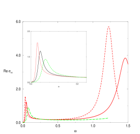
FIG. 1.: $Re\sigma_{xx}(\omega)$ (in units of $b\rho_{m}/\rho_{c}$) as a function of $\omega$ (in units of $\rho_{c}^{3}/\rho_{m}^{2}b$) where $b=cAa^{2}\Delta\rho_{m}^{-2}(e/\hbar)^{3}$ for the case $r_{f}<l_{c}$ for different values of the field $B$ meausred in units of $\rho_{c}^{2}/\rho_{m}b$. The dashed line represents $B=0.33$, the full line $B=0.4$ and the long dashed line $B=0.5$. The inset is a magnification of the pinning peak.

Calculating the resistivities given by $\rho_{\alpha\beta}=-\sigma_{\alpha\beta}/(\sigma_{xx}^{2}+\sigma_{xy}^{2})$ we find that the pinned crystal is indeed insulating i.e., $\rho_{xx}(\omega=0)=\infty$. More importantly, the Hall resisitivity $\rho_{xy}$ turns out to be independent of $\omega$ and $T$ and has the same value as that in the pure system $\rho_{xy}(\omega)={B/\rho_{c}}$. A similar result was argued to hold at $T=0$ in Ref.[14]. At $T>0$ it would be necessary to go beyond the GVM approximation to ascertain whether $\rho_{xy}$ still sticks to its classical value. Indeed the GVM misses soliton like excitations which are known to be important for finite $T$ physics [19, 24].

It is interesting to calculate the field dependences of the above quantities. This is of direct experimental relevance and we use our results to calculate the same. The field dependence of the pinning peak (whose width is naively of $O(\omega_{p})$) is governed by $\Sigma$ whose value is in turn dictated by the relative sizes of the length scales $r_{f}$ and $l_{c}$. Traditionally, in the context of CDW, $\Sigma$ has been related to the Fukuyama-Lee length $R_{a}$ at which relative displacements are of order $a$, as $\Sigma\sim R_{a}^{-2}$. However for the present case such a connection does not hold, because disorder can a priori vary at scales much smaller than $a$ unlike in CDW. This is similar to the situation in vortex systems where pinning is controlled by the Larkin length $R_{c}$, defined as the scale below which the physics of (5) can be described perturbatively by a model where uncorrelated gaussian random forces of strength $\Delta_{f}=\sum_{\bf K}{\bf K}^{2}\Delta_{K}$ act independently on each electron. Within this model $R_{c}$ is given by $\langle[{\bf u}({\bf R}_{c})-{\bf u}({\bf 0})]^{2}\rangle_{f}=\rm{max}[r_{f}^{2},l_{c}^{2}]\equiv\xi^{2}_{0}$. When $R_{c}\gg a$ the crystal is pinned collectively. In this regime using the GVM one finds $\Sigma=cAR_{a}^{-2}(a/\xi_{0})^{6}$. Here $A$ is an overall constant, $R_{a}\sim{{\rho_{m}a^{2}}/{\sqrt{\Delta}}}$ and $\xi_{0}=max[r_{f},l_{c}]$. This corresponds to $\Sigma\sim cR_{c}^{-2}$, implying that $l\sim R_{c}$ (defined above), which shows that the length scale determining the peak in the conductivity is $R_{c}$ and not $R_{a}$. It is important to distinguish between these two lengths since $R_{c}$ can have an explicit dependence on the magnetic field. This yields two very different regimes. One is $r_{f}<l_{c}$, which gives $\Sigma=bB^{3}$ ($b=cAa^{2}\Delta\rho_{m}^{-2}(e/\hbar)^{3}$ ) hence $\omega_{p}(B)\propto B^{2}$ and the pinning peak moves up and broadens with increasing field. This is the case illustrated in Fig. 1 where $Re\sigma_{xx}$ has been plotted for various values of $B$. The second regime is $r_{f}>l_{c}$ leading to a $\Sigma$ independent of $B$ and $\omega_{p}(B)\propto B^{-1}$ . Thus the pinning peak moves towards the origin and gets narrower with increasing field. For CDW in a magnetic field $r_{f}\sim a$ and one is always in the second regime. In these two regimes the height of the pinning peak decreases as $B^{-1}$ with increasing field. For the case $r_{f}\ll l_{c}$, $\omega_{p}$ does not increase indefinitively with $B$, rather there is a crossover to another regime when $R_{c}\sim a$ where single particle pinning effects are dominant. Here the correspondence between $R_{c}$ and $l$ and hence $\Sigma$ no longer holds. One finds then that $\Sigma\propto B^{3\over 2}$ and $\omega_{p}\propto B^{1\over 2}$ provided $l_{c}\gg r_{f}$. In contrast the peak at $\omega_{c}+\omega_{p}$ always moves upwards with increasing $B$. A summary of the results in various regimes is given in Table I.

Another important measurable quantity is the threshold electric field $E_{T}$ necessary for the crystal to slide. This again shows the interplay between $l_{c}$ and $r_{f}$. Using collective pinning arguments [22] one gets $E_{T}={c}R_{c}^{-2}\xi_{0}$ in the regime $R_{c}\gg a$. The threshold field has the same regimes as above and the field dependence are shown in Table I. Note that for $r_{f}>l_{c}$ $E_{T}$ is independent of the field (as for CDW). Since both $E_{T}$ and $\omega_{p}$ are related to $R_{c}$ one has $E_{T}\propto\omega_{p}$ but with a prefactor depending on $\xi_{0}$ and not on $a$ as given by previous CDW estimates. When $R_{c}\leq a$, we enter the regime of single particle pinning. Using $\Sigma\propto B^{3\over 2}$, the threshold field is now $E_{T}\propto\Sigma l_{c}\propto B$ [26]. Finally, due to the variation of $\Sigma$ with the field the dielectric constant $\epsilon$ will exhibit the behaviours shown in Table I. Therefore in addition to detailed frequency measurements of the conductivity, measurements of the $B$ dependences of the dielectric constant could serve as an experimental signature for the WC.

Some of the existing experimental results can be interpreted within our theory. Contrary to previous estimates of the pinning frequency, it allows a scenario where the pinning frequency increases with the field as was seen in recent experiments [17]. A simultaneous increase in $E_{T}$ vs. $B$ is observed which is in qualitative agreement with the above predictions. Our theory also predicts that the Hall resistance takes its classical value which is observed experimentally [8]. However, many problems remain both theoretically and in comparison with experiments. Experimentally the peak height in $\sigma(\omega)$ seems to increase with $B$ which we cannot account for at present. Some experiments [8] seem to report a different behaviour for the conductivity (see however [25]). Finite temperature effects also need to be understood since many experiments are performed in the d.c. limit at $T>0$. Strong disorder effects have also to be understood. Both problems require a careful treatment of the topological defects and solitons which are beyond the scope of the present study. While a phase transition similar to the one occuring in 3d vortex lattices [12] is unlikely in $d=2$, one expects a marked crossover between a weakly pinned WC and a strongly pinned one.

To conclude, we have developed a comprehensive theory for the WC pinned by weak disorder. In addition to detailed frequency dependences of the real and imaginary parts of the conductivites, we have obtained the magnetic field dependences of various dynamical quantities. We find that the magnetic field not only confines the electrons but also plays a crucial role in determining the response of the system to disorder. This dynamical effect, not captured by previous static approximations, allows the possibility of observing novel field dependences.

We thank F.I.B. Williams for enlightening remarks.

Regime	$\Sigma$	$\omega_{p}$	$E_{T}$	$\epsilon$
$r_{f}>l_{c}$	$B^{0}$	$B^{-1}$	$B^{0}$	$B^{0}$
$r_{f}<l_{c}$	$B^{3}$	$B^{2}$	$B^{5\over 2}$	$B^{-3}$
$R_{c}<a$	$B^{3\over 2}$	$B^{1\over 2}$	$B$	$B^{-{3\over 2}}$

TABLE I.: Magnetic field dependences of various dynamical quantities.

REFERENCES

- [1] Laboratoire associé au CNRS.
- [2] E. Wigner, Phys. Rev. 46, 1002(1934).
- [3] E.Y. Andrei, et al, Phys. Rev. Lett. 60,2765(1988).
- [4] R.L Willet et al, Phys. Rev. Lett. 65,633 (1990).
- [5] F.I.B. Williams, et al, Phys. Rev. Lett. 66, 3285 (1991); F. Perruchot thesis, Ecole Polytechnique, Paris, 1995.
- [6] V.J. Goldman et al, Phys. Rev. Lett. 65, 2189 (1990).
- [7] H.C. Manoharan, et al, Phys. Rev. Lett. 77, 1813 (1996).
- [8] V.J. Goldman, M. Shayegan and D. Tsui, Phys. Rev. Lett. 61,881 (1988); T. Sajoto et al, ibid 70, 2321 (1993).
- [9] I.V. Kukushkin and V.B. Timofeev, Phys- Uspekhi 36, 549 (1993).
- [10] A.A. Shashkin et al, Phys. Rev. Lett. 73, 3141 (1994).
- [11] S.C. Zhang, S. Kivelson and D.H. Lee, Phys. Rev. Lett. 69, 1252 (1992).
- [12] T. Giamarchi and P. Le Doussal Phys. Rev. B 52, 1242 (1995).
- [13] H. Fukuyama and P. Lee, Phys. Rev. B 18, 6245 (1978).
- [14] B.G.A. Normand, P.B. Littlewood and A.J. Millis, Phys. Rev. B 46, 3920 (1992); X. Zhue, P.B. Littlewood and A.J. Millis, ibid 50, 4600 (1994).
- [15] U. Wulf, J. Kucera and E. Sigmund Phys. Rev. Lett. 77 2993 (1996).
- [16] Y.P. Li et al, Solid State Comm. 95, 619 (1995).
- [17] C.C. Li et al, preprint; F.I.B. Williams, private communication.
- [18] L. Bonsall and A.A. Maradudin, Phys. Rev. B 15, 1959 (1977).
- [19] T. Giamarchi and P. Le Doussal Phys. Rev. B 53 15206 (1996).
- [20] R. Chitra, T. Giamarchi and P. Le Doussal, manuscript in preparation.
- [21] A.I. Larkin, Zh. Eksp. Teor. Fiz. 58,1466 (1970).
- [22] A.I. Larkin and Y.M. Ovchinnikov, J. Low Temp. Phys. 34, 409 (1979).
- [23] D.R. Nelson and V.M. Vinokur, Phys. Rev. B 48, 13060(1993).
- [24] A. I. Larkin and P. A. Lee Phys. Rev. B 17 1596 (1978).
- [25] They have reported and . However, this linear behaviour in both and violates analyticity properties and more work is needed to clarify this point before a comparison with theory can be made.
- [26] This holds because here the “single particule localization length” (see [12, 23]) . There could be an additional regime where where arguments similar to [23] can be made.