Surface Phason–Polaritons in Charge Density Wave Films

Abstract

The coupled non–radiative excitations of the electromagnetic field and phasons in films with a quasi one–dimensional charge density wave (CDW) are evaluated for P–polarization and CDW conducting axis inside the film. The prominent features are two surface phason–polariton branches extending from the CDW pinning frequency to the frequency of the longitudinal optical phason. These surface phason–polariton states are confined to a finite band of longitudinal wave numbers. Besides surface polaritons, infinite series of guided wave modes are found which extend to large wave numbers. These differences to usual phonon–polaritons are caused by the extreme anisotropy of the electric CDW reponse. At finite temperatures, quasi–particles are thermally excited. Their dissipation leads to polariton damping. Significant level shifts of surface phason–polaritons and guided wave modes are also found. They are due to thermal dressing of the longitudinal optical phason via quasi–particles. The zero and finite temperature results including the case of neglected retardation are displayed in detail.

Keywords: A. thin films, D. charge density waves, D. optical properties.

1 Introduction

The microwave, far infrared, and optical properties of charge density wave (CDW) in quasi one–dimensional conductors (for reviews of CDW physics see [1–3]) are characterized by the large polarization which arises when the CDW is deformed along the chain direction.

At low temperatures, the optical dielectric function for the chain direction is essentially that of a polar crystal – albeit with very different frequency scales due to the heavy Fröhlich mass [4,5]. Together with the extreme anisotropy this leads to peculiar far infrared responses.

The elementary excitations of CDW which couple directly to the electric field are the phasons. Their theoretical discussion has a long history [5–15]. Phasons give rise to phason–polaritons [15] when coupled to the electromagnetic field.

In this paper we study theoretically surface phason–polaritons in CDW films which can now be fabricated [16].

Surface polaritons are well known in conjunction with optical phonons, plasmons and magnons and have been reviewed in [17–20]. The present paper is directly related to the work of Kliewer and Fuchs [21] on surface phonon–polaritons in isotropic films. We generalize their work to anisotropic surface phason–polaritons involving phason dispersion functions calculated in [15]. Uniaxial half–space polariton problems have been considered in [22–24] (cf. also [18]) for other polariton mechanisms and mainly for non–retarded interaction.

We will also investigate the effects of finite temperatures when thermally excited quasi–particles (qp) cause surface phason–polariton damping and level shifts.

It is excepted that surface phason–polaritons can be investigated experimentally by attenuated total reflection (ATR) [25], possibly also by electron energy loss spectroscopy (EELS) [26], and by low energy electron diffraction (LEED) [27]. The guided waves which we find along with the surface phason–polaritons can be measured in microwave cavity experiments similar to those on superconducting films [28].

2 Basic Theory

The bulk results for the dielectric tensor $\epsilon_{ij}({\bf q},\omega)$ of a CDW given as equations (41–44) in [15] refer to long wave lengths $q\ll\xi^{-1}_{0}=\Delta/v_{F}$ ($\Delta$: half gap, $v_{F}$: Fermi velocity) when ${\bf q}$ points into chain direction. The amplitude coherence length $\xi_{0}$ of CDW is rather small away from $T_{c}$. Typical values are $\xi_{0}\approx 3nm$ due to the large value of the half gap $\Delta$. The bulk dielectric functions can thus be used for wave lengths $q<10^{6}$ $cm^{-1}$ and for film thicknesses $2d>30nm$. The geometry under study is shown in Fig. 1.

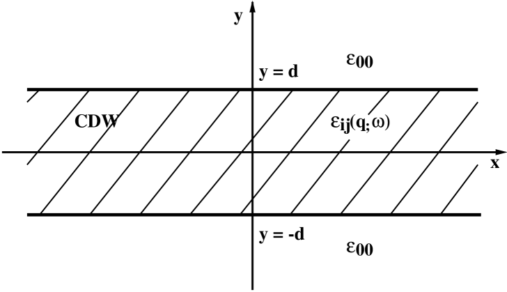
Figure 1: CDW film of thickness $2d$ and with dielectric function $\epsilon_{ij}({\bf q},\omega)$ embedded in a medium of dielectric constant $\epsilon_{00}$. The conducting CDW–axis is chosen as $x$–axis.

The film is embedded in a dielectric medium with dielectric constant $\epsilon_{00}.$ The chain direction of the CDW system lies in the film and is chosen as the x–axis. The corresponding wave number is henceforth called $q$. For $d\rightarrow\infty$ , the limiting case of a half space is obtained. We consider non–radiative electric modes (P–polarization). The electric field inside the film then has components $E_{x}$ and $E_{y}$ and the magnetic field is transverse, lying perpendicular to the conducting axis $(B_{z}\not=0)$. The three–dimensional wave vector then consists of the longitudinal component $q_{x}=q$ and the transverse component $q_{y}\equiv k=-i\alpha$. As shown in [15], the generalization of the solvability relation in [21] to the present anisotropic case is

$$\frac{\omega^{2}}{c^{2}}\left(\epsilon_{xx}\epsilon_{yy}-\epsilon_{xy}^{2}\right)+\alpha^{2}\epsilon_{yy}-q^{2}\epsilon_{xx}+2iq\alpha\epsilon_{xy}=0.$$ (1)

The matching condition for the electromagnetic fields takes on the form

$$\frac{\epsilon_{00}}{\alpha_{0}}=-\left\{\begin{array}[]{c}\coth(\alpha d)\\ \tanh(\alpha d)\end{array}\right\}\quad\left[\frac{\epsilon_{xx}\epsilon_{yy}-\epsilon_{xy}^{2}}{\alpha\epsilon_{yy}+iq\epsilon_{xy}}\right].$$ (2)

The coth–equation gives the high frequency and the tanh–equation the the low frequency branches. In comparison to [15], we changed the notation of the dielectric functions: $\epsilon_{ll}\rightarrow\epsilon_{xx},\epsilon_{t1t1}\rightarrow\epsilon_{yy},\epsilon_{lt}\rightarrow\epsilon_{xy}.$ For surface polaritons, $\alpha$ is positive and defines the decay length in y–direction. The oscillating guided wave modes have imaginary $\alpha=ik$. The light line of the embedding medium is $\alpha_{0}=0$ where $\alpha_{0}$ is defined by

$$\alpha^{2}_{0}=q^{2}-\frac{\omega^{2}}{c^{2}}\epsilon_{00}.$$ (3)

Eliminating $\epsilon_{yy}$ from (2), using (1) gives the simpler formula

$$\frac{\epsilon_{00}}{\alpha_{0}}=-\left\{\begin{array}[]{c}\coth(\alpha d)\\ \tanh(\alpha d)\end{array}\right\}\quad\left[\frac{q\epsilon_{xx}-i\alpha\epsilon_{xy}}{i\omega^{2}\epsilon_{xy}/c^{2}+q\alpha}\right]$$ (4)

for the matching condition.

Equations (1), (3), and (4) determine the desired dispersion relation $\omega=\omega(q)$ by eliminating $\alpha$. This is clearly a complicated task. Enormous simplifications occur in the limit $T\rightarrow 0$ when all $qp$ effects freeze out in the CDW dynamics.

3 CDW Dielectric Tensor at Zero Temperature

The relevant components of the dielectric tensor at zero temperature according to [15] have the simple form

$$\epsilon_{xx}(q,k;\omega)=\epsilon_{0}+\epsilon_{\Delta}\eta_{1}(q)-\frac{c^{2}_{l}\kappa^{2}\eta(q)}{\Omega^{2}(q,k;\omega)},$$ (5)

$$\epsilon_{yy}(q,k;\omega)=\epsilon_{t},\,\,\,\ \epsilon_{xy}=\epsilon_{yx}=0,$$

$$\Omega^{2}\equiv\omega^{2}-\omega^{2}_{0}-c^{2}_{l}q^{2}\eta(q)+c^{2}_{t}\alpha^{2}.$$

Here,

$$\epsilon_{\Delta}=\frac{v^{2}_{F}\kappa^{2}}{6\Delta^{2}_{0}}\gg\epsilon_{0}$$ (6)

is the dielectric constant from virtual transitions across the gap $2\Delta_{0}$ [5].

In (6), $\kappa$ is the Thomas–Fermi wave number and $2\Delta_{0}$ the zero temperature gap. $\epsilon_{\Delta}$ is much larger than the lattice dielectric constant $\epsilon_{0}$ in chain direction. Equation (6) is a valid form for $\omega<\Delta_{0}$. $\eta$ and $\eta_{1}$ are dispersive corrections which become unity for $q\rightarrow 0$ [15]. The phason velocity $c_{l}$ at zero temperature and for the chain direction is given in terms of Fermi velocity $v_{F}$, Peierls phonon frequency $\omega_{Q}$, electron phonon coupling constant $\lambda$, and the half gap $\Delta_{0}$ as [5] :

$$c^{2}_{l}=\frac{\lambda\omega^{2}_{0}}{4\Delta^{2}_{0}}v^{2}_{F}\ll v^{2}_{F}.$$ (7)

The characteristic frequencies of the zero temperature theory are the frequency $\omega_{LO}$ of the longitudinal optical (LO) phason

$$\omega^{2}_{LO}=\frac{c^{2}_{l}\kappa^{2}}{\epsilon_{\Delta}}\equiv\frac{3}{2}\lambda\omega^{2}_{Q},$$ (8)

and the pinning frequency $\omega_{0}$ which usually satisfies

$$\omega_{0}\ll\omega_{LO}.$$ (9)

This is consistent with the clean limit assumption underlying [15]. The frequency $\omega_{LO}$ is of order $10^{13}s^{-1}$ and thus much smaller than usual optical phonon frequencies. For this reason, the transverse lattice dielectric function $\epsilon_{t}$ will be taken as constant in the considered frequency range. This is a strong assumption in view of the possible appearance of bound collective mode resonances in the FIR [29].

A useful dimensionless measure of the wave number $q$ for phason–polaritons then is (c: light velocity)

$$Z=\frac{c^{2}q^{2}}{\omega_{LO}^{2}\epsilon_{t}}.$$ (10)

Z is of order unity for the present purposes, i.e., $q\leq 10^{3}$ $cm^{-1}$. From $c^{2}_{l}q^{2}\equiv\epsilon_{t}\omega^{2}_{LO}Z(c_{l}/c)^{2}$ it is seen that all dispersive effects inside the CDW dielectric functions are irrelevant. Thus one obtains at zero temperature

$$\epsilon_{xx}(\omega)=\epsilon_{\Delta}\left(1-\frac{\omega_{LO}^{2}}{\omega^{2}-\omega_{0}^{2}}\right)\cong\epsilon_{\Delta}\left(\frac{\omega^{2}-\omega_{LO}^{2}}{\omega^{2}-\omega_{0}^{2}}\right),$$ (11)

Equation (11) is identical with the dielectric function of a polar crystal, $\omega_{0}$ playing the role of the transverse optical frequency $\omega_{TO}$ and $\epsilon_{\Delta}$ that of the dielectric constant $\epsilon_{\infty}$. However, (11) refers only to the chain direction. The Lyddane–Sachs–Teller relation

$$\epsilon^{*}=\epsilon_{\Delta}\quad\frac{\omega^{2}_{LO}}{\omega_{0}^{2}},$$ (12)

does not give the static dielectric constant of CDW –which does not exist– but the ”plateau” dielectric constant $\epsilon^{*}$ [30] as explained in [31]. The decisive difference to the usual phonon polariton case is the strong anisotropy $\epsilon_{xx}\not=\epsilon_{t}$ and the different frequency scale. With these simplification the solvability relation (1) reduces to

$$\alpha^{2}=\frac{\epsilon_{xx}}{\epsilon_{t}}\left(q^{2}-\frac{\omega^{2}}{c^{2}}\epsilon_{t}\right).$$ (13)

The matching condition becomes

$$\frac{\epsilon_{00}}{\alpha_{0}}=-\left\{\begin{array}[]{c}\coth(\alpha d)\\ \tanh(\alpha d)\end{array}\right\}\quad\frac{\epsilon_{xx}}{\alpha}.$$ (14)

Equations (3), (13), and (14) completely determine the excitation spectrum.

4 Spectra at Zero Temperature

We will display the phason–polariton spectra in the $W-Z$ plane. $Z$ is given by (10) and the reduced squared frequency $W$ is defined by

$$W=\frac{\omega^{2}}{\omega_{LO}^{2}}.$$ (15)

The existence of surface phason–polaritons requires

$$\epsilon_{t}>\epsilon_{00},$$ (16)

which can be fulfilled. The $W-Z$ quadrant is devided into several regions by the light lines $W=\epsilon_{t}Z/\epsilon_{00}$ ($\alpha^{2}_{0}=0$) and $W=Z$ ($\alpha^{2}=0$) plus horizontal lines $W=1$ and $W=W_{0}$ where $\alpha^{2}$ is also zero due to vanishing of $\epsilon_{xx}$. The quantity $W_{0}$ means $\omega^{2}_{0}/\omega_{LO}^{2}$. Fig. 2 shows this partitioning of the $W-Z$ plane for $\epsilon_{t}=2\epsilon_{00}$. The shaded areas have $\alpha^{2}>0$. They –potentially– could contain surface phason–polaritons. We call them region 1, 2, and 3, respectively. The region to the left of the light line $\alpha_{0}=0$ belongs to $\alpha^{2}_{0}<0$ , i.e., to radiative solutions which we do not consider. The remaining regions I, II, and III have $\alpha^{2}<0.$ They –possibly– contain guided wave solutions. The answers to these questions require detailed investigations of (14), paying special attention to the sign of $\alpha$ and of $\epsilon_{xx}$.

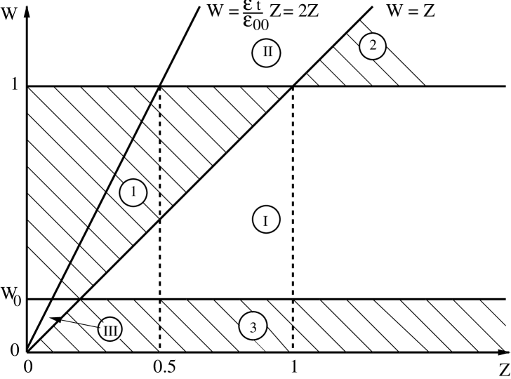
Figure 2: Partitioning of reduced frequency versus wave number plane for the polaritonic response of a CDW film at zero temperature. $W=\omega^{2}/\omega_{LO}^{2}$ measures squared frequency and $Z=c^{2}q^{2}/(\omega_{LO}^{2}\epsilon_{t})$ squared wave number in chain direction. $W=Z$ and $W=2Z$ are the light lines for CDW film and embedding medium, respectively. Regions 1, 2, and 3 sustain surface phason–polaritons ($\alpha^{2}>0$) while regions I, II, and III allow for guided waves ($\alpha^{2}<0$). The region to the left of $W=2Z$ contains the radiative solutions. $W_{0}$ measures CDW–pinning.

We introduce dimensionless parameters according to

$$h=\frac{\epsilon_{t}}{\epsilon_{00}},\,\,\,\,g_{0}=\frac{\epsilon_{\Delta}}{\epsilon_{00}},\,\,\,\,D_{0}=\sqrt{\epsilon_{\Delta}}d\omega_{LO}/c.$$ (17)

For a film of thickness 2d = 1000 nm [16], a typical value of $D_{0}$ would be 0.2.

4.1 Surface Phason–Polaritons

Surface phason–polaritons exist only in region 1 where (14) translates into

$$\sqrt{\frac{(W-W_{0})(W-Z)}{g_{0}(hZ-W)(1-W)}}=\left\{\begin{array}[]{c}\coth X\\ \tanh X,\end{array}\right.X\equiv D_{0}\sqrt{\frac{(1-W)(W-Z)}{W-W_{0}}}.$$ (18)

For each thickness $D_{0}$, there is one surface phason–polariton branch from the coth–equation and one from the tanh–equation separated by the limiting curve for $D_{0}\rightarrow\infty$ which corresponds to the half space problem. The coth–branch ends at the line $W=1$ and the tanh–branch at the line $W=Z$ , as shown in Fig. 3. Both branches start at $(Z=W_{0}/h,W=W_{0})$ and have $W=hZ$ as tangent there. The limiting curve for $D_{0}\rightarrow\infty$ is given implicitly by

$$\left(1-\frac{1}{g_{0}}\right)W^{2}-\left(1+hZ-\frac{Z+W_{0}}{g_{0}}\right)W=\left(\frac{W_{0}}{g}-h\right)Z.$$ (19)

The quantity $g_{0}$ can be much larger than unity. Then the coth–branches (one for each $D_{0}$ ) are squeezed to the $\alpha_{0}=0$ line and thus vanish.

There are no solutions in regions 2 and 3.

Figure 3: Surface phason–polariton branches of a CDW film for several values of the scaled thickness $D_{0}$. The limiting curve $D_{0}\rightarrow\infty$ (dash–dotted line) separates the region of even solutions (to its right) from the region of odd solutions. The quantities $g_{0}$ and $h$ are the high frequency CDW dielectric constants along and transverse to the chains in relation to the embedding medium dielectric constant, respectively.

4.2 Guided Waves

In the regions I, II, and III, $\alpha^{2}$ is negative, i.e., the transverse wave number $k$ is real and the modes oscillate across the film. For imaginary $\alpha$, we find in region I a series of solutions ( p= 0,1,2,3,…)

$$D_{0}\sqrt{\frac{(Z-W)(1-W)}{W-W_{0}}}=p\frac{\pi}{2}+\arctan\sqrt{\frac{(Z-W)(W-W_{0})}{g_{0}(hZ-W)(1-W)}}.$$ (20)

Modes with p = 2m (m= 0,1,2,…) are from the former tanh–equation and those with p = 2m + 1 are from the coth–equation. The $p=0$ mode is the continuation of the corresponding surface phason–polariton. The $p>0$ modes start linearly at $(Z=W_{0}/h,W=W_{0})$. All modes go asymptotically towards $\omega_{LO}$ for large $q$. Fig. 4 shows these guided wave modes. The slopes of the $p>0$ modes near $Z=W_{0}/h$ are given by $D_{0}^{2}(1-W_{0})/(D_{0}^{2}(1-W_{0})+p^{2}(\pi/2)^{2})$ and decrease with increasing order p.

Figure 4: Guided wave modes of region I in a CDW film for a fixed (scaled) thickness $D_{0}=1$ and for several mode numbers $p$. The $p=0$ mode is the continuation of the surface phason–polariton in region 1 (dash–dotted line). The quantities $g_{0}$ and $h$ are the high frequency CDW dielectric constants along and transverse to the chains in relation to the embedding medium dielectric constant, respectively.

Guided waves also exist in region II but not in III. Clearly, there must be a continuation of the coth–surface–polariton branch of region 1 into region II. This is the $n=1$ solution of

$$-D_{0}\sqrt{\frac{(W-Z)(W-1)}{W-W_{0}}}=-n\frac{\pi}{2}+\arctan\sqrt{\frac{(W-Z)(W-W_{0})}{g_{0}(hZ-W)(W-1)}}.$$ (21)

The modes with $n=2m\,(m=1,2,3,\ldots)$ are from the former tanh–equation, the others ($n=2m+1,m=0,1,2,3,\ldots$) are from the coth–equation. All modes with $n\geq 2$ start at discrete points $(Z_{m},W_{m}=hZ_{m})$ on the $\alpha_{0}=0$ line and go asymptotically to the $W=Z$ line. The points $Z_{m}$ solve the equation

$$(h-1)Z_{m}(hZ_{m}-1)=n^{2}\left(\frac{\pi}{2D_{0}}\right)^{2}(hZ_{m}-W_{0}).$$ (22)

These modes, therefore, start at rather high frequencies, the lowest one at $Z_{2}\cong 3$ for our choice $D_{0}=1$ and $h=2$.

Fig. 5 summarizes all our results for the excitation spectra in CDW films at zero temperature.

Figure 5: Survey of all polaritonic excitations of a CDW film: Surface phason polaritons in region 1 (full line) and guided wave modes in regions I and II (broken lines, numbered by integers $p$) for a fixed (scaled) thickness $D_{0}=1$. The quantities $g_{0}$ and $h$ are the high frequency CDW dielectric constants along ($\epsilon_{\Delta}$) and transverse to the chains ($\epsilon_{t}$) in relation to the embedding medium dielectric constant $\epsilon_{00}$, respectively. The limiting curve for $D_{0}\rightarrow\infty$ (dotted line) is the surface phason–polariton of a CDW half space.

4.3 Neglect of Retardation

It is interesting to consider the limit $c\rightarrow\infty$, i.e., when retardation can be neglected. In this limit, only region I survives leaving only guided wave modes. They follow from

$$\sqrt{\tilde{Z}\frac{1-W}{W-W_{0}}}=p\frac{\pi}{2}+\arctan\sqrt{\frac{W-W_{0}}{g_{0}h(1-W)}},\,\,\,\,p=0,1,2,3,....$$ (23)

Here, $\tilde{Z}$ combines wave number q and film thickness 2d according to

$$\tilde{Z}=\frac{\epsilon_{\Delta}}{\epsilon_{t}}(qd)^{2}.$$ (24)

The p = 0 curve for small $\tilde{Z}$ was calculated in [15] and has the characteristic behaviour $\omega\sim\sqrt{q}$ of a two–dimensional plasmon for $\omega_{0}=0$. The modes with $p\geq 1$ are low lying and are acoustic for $\omega_{0}=0$ as shown in Fig. 6.

Figure 6: Non–retarded limit of polaritonic response of CDW films at zero temperature. The wave number scale is $\tilde{Z}=\epsilon_{\Delta}q^{2}d^{2}/\epsilon_{t}$ ($2d$: film thickness). The quantities $g_{0}$ and $h$ are the high frequency CDW dielectric constants along ($\epsilon_{\Delta}$) and transverse to the chains ($\epsilon_{t}$) in relation to the embedding medium dielectric constant $\epsilon_{00}$, respectively. The limiting curve for $D_{0}\rightarrow\infty$ (dotted line) is the surface phason–polariton of a CDW half space.

5 Spectra at Finite Temperatures

At finite temperatures, the expressions for the components of the dielectric tensor become very complicated and contain additional frequency and wave number dependencies. They also depend on elastic and inelastic scattering rates of the $qp$.

At sufficiently high temperatures of about $T_{c}/2$ or higher, the inelastic scattering becomes relevant and the corresponding formulae for $\epsilon_{ij}$ are given as eq. (62) in [15]. Inserting these expressions into the solvability condition (1), a surprising number of cancellations occur. A further significant simplification is the neglect of dispersion in CDW functions by utilizing the argument of Sec. 3. In the end, this simplification amounts to the following approximations for the dielectric tensor

$$\epsilon_{xx}\rightarrow\epsilon_{\Delta}(T)\left[1+\frac{i\omega_{l}(T)}{\omega}-\frac{\omega_{LO}^{2}(T)}{\Omega^{2}(T)}\right],$$ (25)

$$\epsilon_{yy}\rightarrow\epsilon_{t}\left[1+\frac{i\omega_{t}(T)}{\omega}\right],\,\,\,\,\epsilon_{xy}\rightarrow 0.$$

Here, $\omega_{l,t}(T)$ are the dielectric relaxation frequencies of $qp$ for longitudinal and transverse directions, respectively:

$$\omega_{l}(T)=\frac{4\pi\sigma^{(0)}_{l}(T)}{\epsilon_{\Delta}(T)},\,\,\,\,\omega_{t}(T)=\frac{4\pi\sigma^{(0)}_{t}(T)}{\epsilon_{t}}.$$ (26)

The dc–conductivities $\sigma^{(0)}(T)$ are activated and account for the main temperature dependence. They are explicitly given by equation (57) in [15]. We will further assume a quasi–one–dimensional situation when $\omega_{t}\ll\omega_{l}$ holds. Then the solvability relation (1) reduces to

$$\alpha^{2}=\frac{\epsilon_{\Delta}(T)}{\epsilon_{t}}\left[1+\frac{i\omega_{l}(T)}{\omega}-\frac{\omega_{LO}^{2}(T)}{\Omega^{2}}\right]\left\{q^{2}-\frac{\omega^{2}}{c^{2}}\epsilon_{t}\right\}.$$ (27)

This expression must be inserted into (14) to get the spectra $\omega=\omega(q,T)$. It is noted that $\omega$ becomes complex at finite temperatures and that the imaginary part of $\omega$ measures polariton damping.

Temperature dependencies appear not only in $\omega_{l}$ but also in $\omega_{LO},\Omega^{2}$, and $\epsilon_{\Delta}$. The temperature dependent $LO$ phason frequency is given in terms of its zero temperature value $\omega_{LO}$ and the backflow parameter $b_{0}$ as

$$\omega_{LO}^{2}(T)\equiv\frac{c_{l}^{2}(T)\kappa^{2}}{\epsilon_{\Delta}(T)}(1-b_{0})^{2}\equiv\left\{\frac{\epsilon_{\Delta}}{\epsilon_{\Delta}(T)}\left(\frac{\Delta_{0}}{\Delta(T)}\right)^{2}(1-b_{0})^{2}\right\}\omega_{LO}^{2}.$$ (28)

The expression for $\Omega^{2}$ is

$$\Omega^{2}(T)=\omega^{2}+i\omega\gamma_{0}(T)-\omega_{0}^{2}.$$ (29)

The phason damping $\gamma_{0}$ from $qp$ backscattering is defined by equation (60) in [15]. We estimate its value by introducing a cut–off $\nu_{c}\ll k_{B}T$ near the band gap, assuming $\Delta>k_{B}T$ and $\nu_{b}=\nu$ for the $qp$ scattering rates (cf. [15]). This gives

$$\gamma_{0}(T)\approx\frac{\nu}{4\Delta}\,\frac{\lambda\omega_{Q}^{2}}{k_{B}T}\,\left|\ln\left(\frac{\nu_{c}}{k_{B}T}\right)\right|\exp(-\frac{\Delta}{k_{B}T}).$$ (30)

Thus $\Gamma\equiv\gamma_{0}/\omega_{LO}\equiv c_{l}\nu|\ln(\nu_{c}/k_{B}T)|\exp(-\Delta/k_{B}T)/(v_{F}k_{B}T\sqrt{6})\ll 1$ holds and direct phason damping is not important in the frequency and temperature range under study. The phason–polariton damping stems from $qp$ dissipation expressed by $\omega_{l}.$

The temperature dependence of $\epsilon_{\Delta}(T)$ cannot be neglected even when $\Delta=\Delta_{0}$ is considered. It is contained (cf. [15]) in

$$\frac{\epsilon_{\Delta}(T)}{\epsilon_{\Delta}}=\left(\frac{\Delta_{0}}{\Delta(T)}\right)^{2}\frac{3\pi}{2\sqrt{z}}\sum^{\infty}_{n=0}\frac{1}{[(2n+1)^{2}\pi^{2}/(4z)+1]^{5/2}}\equiv\left(\frac{\Delta_{0}}{\Delta(T)}\right)^{2}g_{1}(T).$$ (31)

The quantity $z$ is defined by

$$z=\left(\frac{\Delta}{2k_{B}T}\right)^{2}.$$ (32)

For a qualitative study of finite temperature effects we adopt a simple model in which $\Delta(T)$ is fixed at $\Delta_{0}$. This is not unrealistic for CDW up to $20\%$ $qp$ fraction ($N=0.8$). As in [15] we then find

$$l(T)\equiv\frac{\omega_{l}(T)}{\omega_{LO}}=(1-N)\,8\,\sqrt{\pi}\left(\frac{k_{B}T}{\Delta_{0}}\right)^{3/2}\frac{\sigma_{N}}{\epsilon_{\Delta}(0)\omega_{LO}g_{1}}\equiv\left(\frac{T}{T_{0}}\right)^{3/2}r_{0}(1-N)/g_{1}.$$ (33)

In (33), $\sigma_{N}$ denotes the normal state conductivity. For a reference temperature of $T_{0}=\Delta_{0}/k_{B}=1000K$, the parameter $r_{0}$ is estimated to be of order 10, the value we use in the figures. The expansion of the $qp$ fraction $1-N$ for $\Delta\gg k_{B}T$ is

$$1-N=\sqrt{4\pi\sqrt{z}}\exp(-2\sqrt{z}),$$ (34)

and for $\nu=\nu_{b}$, the backflow parameter $b_{0}$ is approximated by

$$b_{0}=\frac{1}{2\sqrt{z}}(1-N).$$ (35)

5.1 Guided Waves at Finite Temperatures

Using the same scaling as for $T=0$, the matching condition (14) can be written for region I ($p=0,1,2,3,\ldots)$ as

$$D(T)\sqrt{(Z-W)\left[\frac{a(T)-W}{W-W_{0}}-\frac{il(T)}{\sqrt{W}}\right]}=p\frac{\pi}{2}$$ (36)

$$+\arctan\sqrt{\frac{Z-W}{g(T)(hZ-W)\left[(a(T)-W)/(W-W_{0})-il(T)/\sqrt{W}\right]}}.$$

Here, the principal values of the square roots and the $\arctan$ must be taken. The continuation of the $p=0$ solution into region 1 gives the surface phason–polariton from the former tanh–equation. The following parameters which extend zero temperature quantities are used in (36):

$$D(T) = g_{1}(T)\,D_{0},$$ (37)

$$g(T) = g_{1}(T)\,g_{0},$$

$$a(T) = (1-b_{0}(T))^{2}/g_{1}(T).$$

The quantity $a$ reduces to unity for $T\rightarrow 0$. It is a measure of the change of $\omega_{LO}(T)$ with temperature. For small $qp$ concentrations, the decrease of $g_{1}(T)$ with increasing temperature makes $\omega_{LO}(T)$ larger than the zero temperature value $\omega_{LO}$. At even higher temperatures, the backflow parameter $b_{0}$ but also the increased damping $l(T)$ and the decreased order parameter $\Delta(T)$ become relevant for the effective value of $\omega_{LO}(T)$: The LO–phason softens and becomes overdamped. We do not display this region because it is not properly covered by our temperature model.

The non–retarded version of this equation is

$$\sqrt{\tilde{Z}g_{1}\left[\frac{a-W}{W-W_{0}}-i\frac{l}{\sqrt{W}}\right]}=p\frac{\pi}{2}+\arctan\sqrt{\left(hg\left[\frac{a-W}{W-W_{0}}-i\frac{l}{\sqrt{W}}\right]\right)^{-1}}.$$ (38)

Corresponding results are shown in Fig. 7. It is seen that the fundamental mode ($p=0$) is shifted to higher frequencies when the $qp$ fraction increases. This reflects the increase of the LO–phason frequency which has been described above. The guided waves remain underdamped but the imaginary parts of its frequencies do become significant for $N\geq 0.9$. The higher order modes ($p>0$) are much less affected by $qp$.

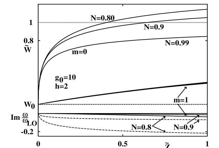
Figure 7: Non–retarded limit of polaritonic response of CDW films at finite temperatures. The wave number scale is $\tilde{Z}=\epsilon_{\Delta}q^{2}d^{2}/\epsilon_{t}$ ($2d$: film thickness) and $\tilde{W}$ means $(Re\omega/\omega_{LO})^{2}$. N is the condensate density and guided wave damping is displayed as $Im\omega/\omega_{LO}<0$. The quantities $g_{0}$ and $h$ are the high frequency CDW dielectric constants along ($\epsilon_{\Delta}$) and transverse to the chains ($\epsilon_{t}$) in relation to the embedding medium dielectric constant $\epsilon_{00}$, respectively.

We like to point out that the surface and bulk phasons for $c\rightarrow\infty$ studied in Section 7.2.3 of [15] appear in a different range than the present phason–polaritons, namely at much smaller frequencies, larger wave numbers, and higher temperatures ($\omega_{l}>\omega_{LO}$). Neglect of internal CDW–dispersion is then not permitted.

5.2 Surface Phason–Polaritons at Finite Temperatures

Finally, we study the surface phason–polaritons in region 1 starting from the appropriate formulae for region 1:

$$\sqrt{\frac{W-Z}{g(T)(hZ-W)\left[(a(T)-W)/(W-W_{0})-il(T)/\sqrt{W}\right]}}=\left\{\begin{array}[]{c}\coth X(T)\\ \tanh X(T),\end{array}\right.$$ (41)

$$X(T)\equiv D(T)\sqrt{(W-Z)\left[\frac{a(T)-W}{W-W_{0}}-\frac{il(T)}{\sqrt{W}}\right]}.$$

Unfortunately, these transcendental equations are difficult to solve, even on a computer. Therefore, we limit ourselves to the half space case $D(T)\rightarrow\infty$ when a simple fifth order polynomial in the frequency $\omega\propto\sqrt{W}$ remains:

$$g(T)(hZ-W)\left[\sqrt{W}(a(T)-W)-il(T)(W-W_{0})\right]=\sqrt{W}(W-W_{0})(W-Z).$$ (42)

Figure 8: Surface phason–polaritons in a thick CDW film at finite temperatures. $\tilde{W}$ means $(Re\omega/\omega_{LO})^{2}$. N is the condensate density and polariton damping is displayed as $5Im\omega/\omega_{LO}<0$. The quantities $g_{0}$ and $h$ are the high frequency CDW dielectric constants along and transverse to the chains in relation to the embedding medium dielectric constant, respectively.

Its surface phason–polariton solutions are shown in Fig. 8 for several $qp$ densities. In contrast to usual surface phonon–polaritons, the $qp$ cause a significant temperature variation of the surface polariton frequencies. The surface phason–polaritons are underdamped for the $qp$ densities considered.

6 Summary

The strong anisotropy of the polar crystal like optical response of quasi one–dimensional CDW has a distinguished influence on the coupled excitations of the electromagnetic field and CDW phasons. These excitations are grouped into surface phason–polaritons and guided wave modes and their frequencies are considerably smaller than the corresponding excitations involving optical phonons. This is due to the large effective mass of CDW which leads to a low frequency of the longitudinal optical phason. At finite temperatures, quasi–particles cause damping and considerable level shifts of both surface phason polaritons and guided wave modes. We have given a complete discussion of these surface phason–polaritons and guided wave modes for the case of P–polarization and for the conducting CDW axis lying inside the film.