Power Law Scaling for a System of Interacting Units with Complex Internal Structure

Abstract

We study the dynamics of a system composed of interacting units each with a complex internal structure comprising many subunits. We consider the case in which each subunit grows in a multiplicative manner. We propose a model for such systems in which the interaction among the units is treated in a mean field approximation and the interaction among subunits is nonlinear. To test the model, we identify a large data base spanning 20 years, and find that the model correctly predicts a variety of empirical results.

PACS numbers: 05.40.+j, 02.50.-r, 05.70.Ln, 02.50.Ey, 05.20.-y, 89.90.+n

In the physical sciences, power law scaling is usually associated with critical behavior, thus requiring a particular set of parameter values. For example, in the Ising model there is a particular value of the strength of the interaction between the units composing the system that generates correlations extending throughout the entire system and leads to power law distributions [1]. In the social and biological sciences, there also appear examples of power law distributions (incomes [2], city sizes [3], extinction of species [4], bird populations [5], heart dynamics [6]). However, it is difficult to imagine that for all these diverse systems, the parameters controlling the dynamics spontaneously self-tune to their critical values.

In this Letter, we raise an alternative mechanism by asking how power law distributions can emerge even in the absence of critical dynamics. The guiding principles for our approach, to be justified below, are: (i) the units composing the system have a complex evolving structure (e.g., the companies competing in an economy are composed of divisions, the cities in a country competing for the mobile population are composed of distinct neighborhoods, the population of some species living in a given ecosystem might be composed of groups living in different areas), and (ii) the size of the subunits composing each unit evolve according to a random multiplicative process.

Fortunately, for one of the examples listed above, there is a wealth of quantitative data, and here we focus on a large database giving the time evolution of the size of companies [7]. In an economy, the units composing the entire system are the competing companies. In general, these companies have a complex internal structure, with each company composed of divisions (the subunits of each unit). It has been proposed that the evolution of a company’s size is described by a random multiplicative process with variance independent of the size, and that each company can be viewed as a structureless unit [8]. However, later studies [9, 10, 11, 12, 13, 14, 15] reveal that the dynamics of real companies are not fully consistent with the simplified picture of Ref. [8].

We develop here a model that dynamically builds a diversified, multi-divisional structure, reproducing the fact that a typical company passes through a series of changes in organization, growing from a single-product, single-plant company, to a multi-divisional, multi-product company [16]. The model reproduces a number of empirical observations for a wide range of values of parameters and provides a possible explanation for the robustness of the empirical results. Due to our encouraging results for the case of company growth, our model may offer a generic approach to explain power law distributions in other complex systems.

The model, illustrated in Fig. 1, is defined as follows. A company is created with a single division, which has a size $\xi_{1}(t=0)$. The size of a company $S\equiv\Sigma_{i}\xi_{i}(t)$ at time $t$ is the sum of the sizes of the divisions $\xi_{i}(t)$ comprising the company. We define a minimum size $S_{\rm min}$ below which a company would not be economically viable, due to the competition between companies; $S_{\rm min}$ is a characteristic of the industry in which the company operates. We assume that the size of each division $i$ of the company evolves according to a random multiplicative process [8]. We define

$$\Delta\xi_{i}(t)\equiv\xi_{i}(t)~{}\eta_{i}(t)\,,$$ (1)

where $\eta_{i}(t)$ is a Gaussian-distributed random variable with zero mean and standard deviation $V$ independent of $\xi_{i}$. The divisions evolve as follows:

• If $\Delta\xi_{i}(t)<S_{\rm min}$, division $i$ evolves by changing its size, and $\xi_{i}(t+1)=\xi_{i}(t)+\Delta\xi_{i}(t)$. If its size becomes smaller than $S_{\rm min}$ — i.e. if $\xi_{i}(t+1)<S_{\rm min}$ — then with probability $p_{a}$, division $i$ is “absorbed” by division $1$. Thus, the parameter $p_{a}$ reflects the fact that when a division becomes very small it will

  

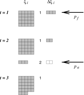
  FIG. 1.: Schematic representation of the time evolution of the size and structure of a company. We choose $S_{\rm min}=2$, and $p_{f}=p_{a}=1.0$. The first column of full squares represents the size $\xi_{i}$ of each division, and the second column represents the corresponding change in size $\Delta\xi_{i}$. Empty squares represent negative growth and full squares positive growth. We assume, for this example, that the company has initially one division of size $\xi_{1}=25$, represented by a $5\times 5$ square. At $t=1$, division 1 grows by $\Delta\xi_{1}=3$. A new division, numbered 2, is created because $\Delta\xi_{1}>S_{\rm min}=2$, and the size of division 1 remains unchanged, so for $t=2$, the company has 2 divisions with sizes $\xi_{1}=25$ and $\xi_{2}=3$. Next, divisions $\xi_{1}$ and $\xi_{2}$ grow by $2$ and $-2$, respectively. Division $2$ is absorbed by division $1$, since otherwise its size would become $\xi_{2}=3-2=1$ which is smaller than $S_{\rm min}$. Thus, at time $t=3$, the company has only one division with size $\xi_{1}=25+2+1=28$. Note that if division $1$ would be absorbed, then division $2$ would absorb division $1$ and would then be renumbered $1$. If, division $1$ is absorbed and there are no more divisions left, the company “dies.”

  no longer be viable due to the competition between companies.

• If $\Delta\xi_{i}(t)>S_{\rm min}$, then with probability $(1-p_{f})$, we set $\xi_{i}(t+1)=\xi_{i}(t)+\Delta\xi_{i}(t)$. With a probability $p_{f}$, division $i$ does not change its size — so that $\xi_{i}(t+1)=\xi_{i}(t)$ — and an altogether new division $j$ is created with size $\xi_{j}(t+1)=\Delta\xi_{i}(t)$. Thus, the parameter $p_{f}$ reflects the tendency to diversify: the larger is $p_{f}$, the more likely it is that new divisions are created.

The dynamics are thus controlled by four parameters: $S_{\rm min}$, $V$, $p_{a}$, and $p_{f}$; $S_{\rm min}$ just sets the scale, so the results of the model do not depend on its value. We assume that there is a broad distribution of values of $S_{\rm min}$ in the system because companies in different activities will have different constraints.

In Fig. 2, we compare the predictions of the model for the distribution of company sizes with the empirical data [15]. We find similar results for a wide range of parameters: $V=0.1-0.2$, $p_{a}=0.01-1$, and $p_{f}=0.1-1.0$. We define one “year” to be $\ell$ iterations of our rules applied to each company, and we find no significant dependence of the results on the value of $\ell$ for $\ell=20,30$ or $50$.

FIG. 2.: Probability density of the logarithm of company size for the model and for US publicly-traded manufacturing firms in the 1994 “Compustat” data base. To obtain these results, we assume that $S_{\rm min}$ is drawn from a truncated log-normal distribution with average value $5\times 10^{5}$. The numerical simulations were performed with parameters $V=0.15$, $p_{f}=0.8$, $p_{a}=0.05$, and $\ell=50$ (for these parameter values, the actual probability of a new division being created per division and per iteration is approximately $0.01$).

It is common to study the logarithm of the one-year growth rate, $r_{1}\equiv\ln R_{1}$, where $R_{1}\equiv S(y+1)/S(y)$, and $S(y)$ and $S(y+1)$ are the sizes of the company in the years $y$ and $y+1$. The empirical distribution of $r_{1}$ for companies with size $S$ is consistent with an exponential form [15]

$$p(r_{1}|S)=\frac{1}{\sqrt{2}\sigma_{1}(S)}\exp\left(-{\sqrt{2}\,|r_{1}-\bar{r}_{1}|\over\sigma_{1}(S)}\right)\,,$$ (2)

where $\bar{r}_{1}$ represents the average growth rate. Moreover, the standard deviation $\sigma_{1}(S)$ is consistent with a power law form

$$\sigma_{1}(S)\sim S^{-\beta},$$ (3)

and for US manufacturing companies, $\beta\approx 0.2$ [15]. Figure 3a displays $p(r_{1}|S)$, and is quite similar in form to empirical results [15]. Figure 3b compares $\sigma_{1}(S)$ with the empirical data of Ref. [15]: for both, Eq. (3) holds with $\beta=0.17\pm 0.03$. Equations (2)–(3) allow us to scale the growth rate distributions for different company sizes (Fig. 3c).

We next address the question of the structure of a given company. To this end, we calculate the probability density $\rho_{1}(\xi_{i}|S)$ to find a division of size $\xi_{i}$ in a company of size $S$. For the model, we find that the distribution $\rho_{1}$ is peaked at a maximum which scales as $S^{\alpha}$. Hence, we make the hypothesis that $\rho_{1}$ obeys the scaling relation

$$\rho_{1}(\xi_{i}|S)\sim S^{-\alpha}f_{1}\left(\xi_{i}/S^{\alpha}\right)\,.$$ (4)

This hypothesis is confirmed by the scaling plot of Fig. 4a. We find $\alpha=0.66\pm 0.05$ from plotting the average value of $\xi_{i}$ against $S$. The same value of $\alpha$ leads to the best scaling plot.

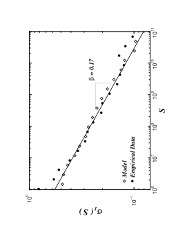
FIG. 3.: (a) Probability density of one-year growth rates for firms with different sizes. The values of the parameters are the same as in Fig. 2. The distributions are tent-shaped, as for the empirical data [15], consistent with an exponential distribution. (b) Dependence of the standard deviation of the growth rates on company size. Shown are the predictions of the model and the empirical results. The straight line with slope $0.17$ is a least square fit to the predictions of the model. (c) Probability density of one-year growth rates for different company sizes plotted in scaled variables.

Next, we make the hypothesis that the probability density $\rho_{2}(N|S)$ to find a company with size $S$ composed of $N$ divisions, obeys the scaling relation

$$\rho_{2}(N|S)\sim S^{-(1-\alpha)}f_{2}\left(N/S^{1-\alpha}\right)\,.$$ (5)

In writing (5), we use the fact that from (4) the characteristic size of a typical division scales as $S^{\alpha}$, so that the typical number of divisions in a company is $S/S^{\alpha}\sim S^{1-\alpha}$. Figure 4b shows that the results of the model are consistent with the scaling relation (5), with the same value of the scaling exponent $\alpha$ used in Fig. 4a.

The results described by Eqs. (4)-(5) are in qualitative agreement with empirical studies [10, 14] that show larger firms to be more diversified. Moreover, Eqs. (4)-(5) lead to the simple scaling law

$$\beta=(1-\alpha)/2\,,$$ (6)

which can be tested. For $\alpha=0.66\pm 0.05$, (6) predicts $\beta=0.17\pm 0.03$, in remarkable agreement with our independent calculation of $\beta$.

FIG. 4.: (a) “Data collapse” of the conditional probability density $\rho_{1}$; the data fall onto a single curve corresponding to the scaling form (4). (b) “Data collapse” of the conditional probability density $\rho_{2}$; the data fall onto a single curve corresponding to the scaling form (5).

We find that the predictions of the model are only weakly sensitive to the parameter values, which perhaps is the reason why firms operating in quite different industries are described by very similar empirical laws. Accordingly, we conjecture that the scaling laws found for US manufacturing firms [15] also hold for other countries, such as Japan, with $\beta\approx 0.2$; this conjecture is currently being tested with empirical data [17].

The present model rests on a small number of assumptions. The two key assumptions are: (i) Firms tend to organize themselves into multiple divisions once they achieve a certain size. This assumption holds for many modern corporations [16]. (ii) Growth rates of different divisions are independent of one another. For an economist, the latter is perhaps the stronger of the two assumptions. We find that correlations in the growth rates of divisions within a same company, even weak correlations, lead to $\beta\approx 0$. Thus, we confirm that it is the assumption of independence among the growth rates that reproduces the empirical findings of Refs. [15].

There are two features of our results that are perhaps surprising. First, although firms in our model consist of independent divisions, we do not find $\beta=1/2$. To understand why $\beta<1/2$, suppose that the distribution of $s_{m}\equiv\ln S_{\rm min}$ is a Dirac $\delta$-function. Although this assumption is unrealistic, it leads to an understanding of the underlying mechanisms in the model. For this case, we find (i) that the distribution of company sizes is still close to log-normal, with a width $\cal W$ which is a function of the parameters of the model and, (ii) that the number of divisions increases linearly with size, so $\alpha=0$ and $\beta=1/2$. Then, by integration over $s_{m}$, we can estimate the value of $\beta$ for the case of a broader distribution of $s_{m}$. Suppose that $s_{m}$ follows some arbitrary distribution with width $\cal D$. Averaging $\sigma_{1}^{2}(S)$ over this distribution, we find $\beta={\cal W}/2({\cal D}+{\cal W})$. For a wide range of the values of the model’s parameters, ${\cal D}>{\cal W}$, and we find that $\beta$ is remarkably close to the empirical value $\beta\approx 0.2$.

Second, the distribution $p(r_{1}|S)$ is not Gaussian but “tent” shaped. We find this result arises from the integration of nearly-Gaussian distributions of the growth rates over the distribution of $S_{\rm min}$. For large values of $|r_{1}|$, the saddle point approximation gives $p(r_{1}|S)\sim\exp(-\log^{2}|r_{1}|)$, which decays slower than exponentially, in qualitative agreement with the model’s predictions and with empirical observations. For $|r_{1}|\ll 1$, $p(r_{1}|S)$ is approximately Gaussian, while for intermediate values of $|r_{1}|$, the distribution decays exponentially. Our analytical predictions are in agreement with the model and with empirical results.

The model leads to a number of conclusions. First, it suggests the deviations in the empirical data from predictions of the random multiplicative process may be explained (i) by the diversification of firms, i.e., firms are made up of interacting subunits; and (ii) by the fact that different industries have different underlying scales, i.e., there is a broad distribution of minimum scales for the survival of a unit (for example, a car manufacturer must be much larger than a software company).

Second, the model suggests a possible explanation for the common occurrence of power law distributions in complex systems. Our results suggest that the empirically observed power law scaling does not require some “critical state” of the system, but rather can arise from a interplay between random multiplicative growth and the complex structure of the units composing the system. Here we addressed the case in which the interactions between the units can be treated in a mean field way through the imposition of a minimum size for the subunits. We believe that more complex interactions will still lead to power law scaling, and that our model may offer a possible framework for the the study of complex systems.

REFERENCES

- [1] For self-organized criticality [P. Bak, C. Tang, and K. Wiesenfeld, Phys. Rev. Lett. 59, 381 (1987)] the parameters controlling the dynamics spontaneously self-tune toward the critical values.
- [2] V. Pareto, Cours d’Economie Politique, Vol. 2 (1897).
- [3] G. K. Zipf, Human Behavior and the Principle of Least Effort (Addison-Wesley, Cambridge MA, 1949).
- [4] N. Eldredge and S. J. Gould, Nature 332, 211 (1988) and references therein.
- [5] T. H. Keitt (private discussion, Santa Fe Institute, 1997).
- [6] C.-K. Peng et al., Phys. Rev. Lett. 70, 1343 (1993).
- [7] Specifically, for each company in the “Compustat” database of all US publicly-traded firms, it is listed a variety of economic variables such as sales, number of employees, assets, etc. In this work, we use the generic term “size” to mean any of these quantities because a precious study [15] showed them to scale in an identical way.
- [8] R. Gibrat, Les Inégalités Economiques (Sirey, Paris, 1931).
- [9] For a review, see J. Sutton, J. Eco. Literature 35, 40 (1997) and refs. therein.
- [10] M. Gort, Diversification and Integration in American Industry (Princeton University Press, Princeton, 1962).
- [11] Y. Ijiri and H. A. Simon, Skew Distributions and the Sizes of Business Firms (North Holland, Amsterdam, 1976).
- [12] D. S. Evans, J. Pol. Econ. 95, 657 (1987); B. H. Hall, J. Indust. Econ. 35, 583 (1987).
- [13] S. J. Davis, J. Haltiwanger, and S. J. Schuh, Job Creation and Destruction (MIT Press, Cambridge, Massachusetts, 1996).
- [14] B. Jovanovic, Brookings Papers on Economic Activity: Microeconomics (1), 197 (1993).
- [15] M. H. R Stanley et al., Nature 379, 804 (1996); L. A. N. Amaral et al., J. Phys. I France 7, 621 (1997).
- [16] A. Chandler, Strategy and Structure (MIT Press, Cambridge, 1962); O. E. Williamson in Handbook of Industrial Organization Vol. 1, eds. R. Schmalensee and R. Willig, 135 (North Holland, Amsterdam, 1989).
- [17] H. Takayasu (to be published); H. Takayasu, A.-H. Sato, and M. Takayasu, “Stable Infinite Variance Fluctuations in Randomly Amplified Langevin Systems,” Phys. Rev. Lett. (to appear).