[

Phase Separation in One-Dimensional Driven Diffusive Systems

Abstract

A driven diffusive model of three types of particles that exhibits phase separation on a ring is introduced. The dynamics is local and comprises nearest neighbor exchanges that conserve each of the three species. For the case in which the three densities are equal, it is shown that the model obeys detailed balance. The Hamiltonian governing the steady state distribution in this case is given and is found to have long range asymmetric interactions. The partition sum and bounds on some correlation functions are calculated analytically demonstrating phase separation.

]

Driven diffusive systems have been a subject of extensive studies in recent years [1, 2]. Being driven by an external field, these systems are governed by dynamics which generically does not obey detailed balance, leading to steady states with non-vanishing currents. This class of systems provides a relatively simple framework within which collective phenomena far from thermal equilibrium may be studied [3, 4].

Theoretical studies of models of driven diffusive systems reveal some basic differences between phase transitions taking place under equilibrium and non-equilibrium conditions. For example it is well known that phase transitions and spontaneous symmetry breaking are not expected to take place in one dimensional ($1d$) systems in thermal equilibrium at finite temperatures, as long as the interaction in the system is short range. Recently it has been demonstrated that this is not the case in systems far from thermal equilibrium [5]. Indeed, a simple example of an open system with non-conserved order parameter at the boundaries was shown to exhibit spontaneous symmetry breaking [4].

A closely related problem is that of phase separation. An interesting question is whether $1d$ homogeneous systems (i.e. with no boundary effects as in a ring geometry) are capable of exhibiting phase separation, in cases where conserving dynamics is involved. It has been shown that inhomogeneities, such as defect sites or particles may trigger the formation of macroscopic regions of high density bound to the defect [6]. Recent numerical studies of a model associated with sedimentation of colloidal crystals have suggested that phase separation may even occur in homogeneous non-equilibrium systems [7].

Phase separation is accompanied by coarsening phenomena in which the typical domain size grows indefinitely with time [8]. Examples of equilibrium $1d$ systems with local dynamics which exhibit coarsening are the zero temperature limit of kinetic Ising models and the noiseless Landau-Ginzburg equation. However these systems do not coarsen at finite temperature.

In the present Letter we introduce a simple model of phase separation in a $1d$ driven diffusive system. This is a model of $3$ species of particles on a ring in which nearest neighbors on the lattice are exchanged with specific rates. Thus the dynamics is local, fully stochastic and conserves each of the three species. It is shown that for the special case in which the average densities of the three species are equal, the dynamics obeys detailed balance. In this case the steady state distribution is shown to be given by a Hamiltonian which has long range asymmetric interactions. The phase separation which takes place in the model is explicitly demonstrated for this case. It is argued that phase separation takes place in the general case where the densities of the three species are unequal and that the typical domain size coarsens as $\ln t$. The model is easily generalized to $n$ species and phase separation is found provided $n>2$.

A. Definition of the model: The model is defined on a $1d$ lattice of length $N$ with periodic boundary conditions. Each site is occupied by either an $A$, $B$, or $C$ particle. The evolution is governed by random sequential dynamics defined as follows: at each time step two neighboring sites are chosen randomly and the particles of these sites are exchanged according to the following rates

(1)

The rates are cyclic in $A$, $B$ and $C$ and conserve the number of particles of each type.

Consider a system with $N_{A}$ particles of type $A$, $N_{B}$ of type $B$, and $N_{C}$ of type $C$. For $q=1$ the particles undergo symmetric diffusion and the system is disordered. However for $q\neq 1$ the particle exchange rates are biased. Since the model is invariant, for example, under the exchange $A\to B$ and $q\to 1/q$, it is sufficient to consider $q<1$. In this case the bias drives, say, an $A$ particle to move to the left inside a $B$ domain, and to the right inside a $C$ domain. Therefore, starting with an arbitrary initial configuration, the system reaches after a relatively short transient time a state of the type $\ldots AABBCCAAAB\ldots$ in which $A,B$ and $C$ domains are located to the right of $C$, $A$ and $B$ domains, respectively. Due to the bias $q$, the domain walls $\ldots AB\ldots$, $\ldots BC\ldots$, and $\ldots CA\ldots$, are stable, and configurations of this type are long lived. In fact, the domains in these configurations diffuse into each other and coarsen on a time scale of the order of $q^{-L}$, where $L$ is a typical domain size in the system. This leads to the growth of the typical domain size as $(\ln t)/|\ln q|$. Eventually the system phase separates into three domains of the different species of the form $A\ldots AB\ldots BC\ldots C$. A finite system does not stay in such a state indefinitely. For example, the $A$ domain breaks up into smaller domains in a time of order $q^{-min\{N_{B},N_{C}\}}$. In the thermodynamic limit, however, when the density of each type of particle is non vanishing, the time scale for the break up of extensive domains diverges and we expect the system to phase separate. Generically the system supports particle currents in the steady state. This can be seen by considering, say, the $A$ domain in the phase separated state. The rates at which an $A$ particle traverses a $B$ ($C$) domain to the right (left) is of the order of $q^{N_{B}}$ ($q^{N_{C}}$). The net current is then of the order of $q^{N_{B}}-q^{N_{C}}$, vanishing exponentially with $N$. This simple argument suggests that for the special case $N_{A}=N_{B}=N_{C}$ the current is zero for any system size.

In the following, we show that the dynamics of the model satisfies detailed balance for the special case $N_{A}=N_{B}=N_{C}$. The Hamiltonian governing the steady state distribution is found to have long range interactions. It is demonstrated that phase separation takes place in the thermodynamic limit. The simple considerations given above indicate that phase separation exists even when the number of particles of the three species are not equal.

B. Special case, $N_{A}=N_{B}=N_{C}$ : We specify a configuration by the set of numbers $\{X_{i}\}=\{A_{i},B_{i},C_{i}\}$, where $A_{i}$, $B_{i}$ and $C_{i}$ are equal to one if site $i$ is occupied by particle $A$, $B$ or $C$ respectively and zero otherwise. We show that the dynamics satisfies detailed balance with respect to the Hamiltonian ${\cal H}$ given by:

$${\cal H}(\{X_{i}\})=\sum_{i=1}^{N-1}\sum_{j=i+1}^{N}[C_{i}B_{j}-C_{i}A_{j}+B_{i}A_{j}].$$ (2)

So that, in the steady state the probability of finding the system in a configuration $\{X_{i}\}$ is given by:

$$W_{N}(\{X_{i}\})=Z_{N}^{-1}q^{{\cal H}(\{X_{i}\})},$$ (3)

where the partition sum is given by $Z_{N}=\sum_{\{X_{i}\}}q^{{\cal H}(\{X_{i}\})}$ and the sum runs over all states in which $N_{A}=N_{B}=N_{C}$. Although expression (2) for the Hamiltonian is not manifestly translationally invariant, a form that is clearly invariant under translations can be simply obtained from (2) but is less convenient for our purposes.

Before proving Eqs.(2,3) let us make a few comments. The $N$-fold degenerate zero energy ground states of the Hamiltonian (2) comprise the fully separated configuration $A\ldots AB\ldots BC\ldots C$ and any translation of this configuration. Starting from a ground state, any other configuration may be obtained by successive permutations of nearest neighbor particles. The energy of such configuration may be calculated by noting that any particle exchange against the bias costs one unit of energy while an exchange in the direction of the bias results in a gain of one unit. The maximal energy of this Hamiltonian is $N^{2}/9$ and corresponds to a fully separated state $A\ldots AC\ldots CB\ldots B$. It is of interest to note that although the dynamics defined in (1) is local, the resulting Hamiltonian (2) is long range, in which each particle interacts with all other particles. Also the interactions are asymmetric in the sense that the Hamiltonian is not invariant under space inversion. The temperature of the system is given by $T=1/|\ln q|$.

To prove Eqs.(2,3) one can check that $W_{N}(\{X_{i}\})$ satisfies detailed balance with respect to the dynamics (1). For example it is easy to see that an exchange of particles in the bulk of the lattice $\ldots AB\ldots\rightarrow\ldots BA\ldots$ satisfies $qW_{N}(...AB...)=W_{N}(...BA...)$. Similarly, particle exchange between site $1$ and $N$, say, $A\ldots C\rightarrow C\ldots A$ satisfies $qW_{N}(A......C)=W_{N}(C......A)$, as long as $N_{A}=N_{B}=N_{C}$. Note that when the three densities are not equal, the system supports a current, and thus it cannot satisfy detailed balance.

In order to demonstrate phase separation it is sufficient to show that for large finite $k$ the two point density correlation function satisfies

$$\lim_{N\to\infty}(\langle A_{1}A_{k}\rangle-\langle A_{1}\rangle\langle A_{k}\rangle)>0\;.$$ (4)

In our case this implies $\lim_{N\to\infty}\langle A_{1}A_{k}\rangle>1/9$ for large $k$. In fact we show below that in the limit of large $N$ and for any finite $k$:

$$\langle A_{1}A_{k}\rangle=1/3-O(1/N),$$ (5)

demonstrating the existence of phase separation in the model. This result indicates that the phase separation is complete, in the sense that the probability of finding, say, a $B$ or a $C$ particle a large distance inside the $A$ domain vanishes in the thermodynamic limit.

We proceed by first calculating the partition sum, $Z_{N}$, showing that for $q<1$ and to leading order in $N$

$$Z_{N}=N/\left[(q)_{\infty}\right]^{3},$$ (7)

where

$$(q)_{\infty}=\lim_{n\rightarrow\infty}(1-q)(1-q^{2})\ldots(1-q^{n}).$$ (8)

The partition sum for $q>1$ is obtained by replacing $q$ by $1/q$ in this expression. Note that the partition sum (Phase Separation in One-Dimensional Driven Diffusive Systems ) is proportional to $N$ rather than being exponential in $N$. This is a consequence of the long range interactions; low energy excitations are localized about the domain boundaries and their degeneracy does not increase with system size (in contrast to short range models). At $q=1$, however, all configurations are equally probable and the partition sum is exponential in $N$.

The calculation of the partition sum is greatly simplified by noting that configurations with energy larger than $aN$, where $a>0$ is a constant, can be neglected in the thermodynamic limit. Here we show that this is the case for $q<(1/3)^{1/a}$. A more detailed analysis completes the proof for all $q\neq 1$ [10]. Consider the sum $Z_{m>aN}=\sum_{m=aN+1}^{N^{2}/9}D(m)q^{m}$, where $D(m)$ is the number of states of energy $m$. Noting that $D(m)$ is bounded from above by the total number states which in turn is bounded by $3^{N}$, one finds that $Z_{m>aN}$ decays exponentially with $N$ as long as $q<(1/3)^{1/a}$. Hence, the partition sum may be replaced by the truncated one as long as exponentially small corrections in $N$ are of no interest.

To calculate the truncated partition sum we note that states with energy $m<N/3-1$, may be uniquely decomposed into $N$ disjoint sets, where each set corresponds to one of the $N$ ground states of the system. Any state within a given set may be obtained from the corresponding ground state by successive permutations of nearest neighbor particles, in a way that the energy always increases along the path of intermediate states.

The sets are labeled by $l=1\ldots N$, the position of the rightmost $A$ particle in the $A$ domain in the ground state configuration of that set (Fig.(1)). Due to the translational invariance of the model the partition sum can be written as $Z_{N}=N{\cal Z}+e^{-O(N)}$ where ${\cal Z}$ is the partition sum obtained by summing over one of the $N$ sets of configurations.

FIG. 1.: The $l=5$ ground state for an $N=21$ system.

We now turn to calculating ${\cal Z}$. Consider an excitation of energy $m$ created only at one domain boundary, say $AB$. The excitation can be formed by one or more $B$ particles moving into the $A$ domain (equivalently $A$ particles moving into the $B$ domain). A moving $B$ particle may be considered as a walker. The energy of the system increases linearly with the distance traveled by the walker inside the $A$ domain. An excitation of energy $m$ at the $AB$ boundary is formed by $j$ walkers passing a total distance of $m$. Hence, the total number of states of energy $m$ at the $AB$ boundary is equal to the number of ways $P(m)$ of partitioning an integer $m$ into a sum of (positive) integers. When considering all three interfaces in the ground state, the number of states composed of excitations of energy $m_{i},i=1,2,3$ at the three interfaces is given by $P(m_{1})P(m_{2})P(m_{3})$. Note that since only excitations with total energy smaller than $N/3-1$ are considered, a walker can not travel from one boundary to another, and local excitations at the three boundaries are independent. The partition sum ${\cal Z}$, after taking the thermodynamic limit, is given by

$${\cal Z}=\sum_{m=0}^{\infty}q^{m}\sum_{m_{i}=0}^{m}\!P(m_{1})P(m_{2})P(m_{3})\delta_{m_{1}+m_{2}+m_{3},m}.$$ (9)

This sum may be rewritten as

$${\cal Z}=(\sum_{m=0}^{\infty}q^{m}P(m))^{3}.$$ (10)

Using the classical result for the generating function of $P(m)$ [9], attributed to Euler, we obtain Eqs.(Phase Separation in One-Dimensional Driven Diffusive Systems ). Note that excitations of energy up to $N/3-2$ are properly accounted for. Once excitations of greater energy are considered, triplets of the form $\ldots ABC\ldots$ can be formed. These triplets can be moved around the lattice with no energy cost so that the degeneracy is not accounted for correctly in Eqs.(Phase Separation in One-Dimensional Driven Diffusive Systems ). However, our results above imply that these contributions are unimportant for $q<(1/3)^{3}$. A more detailed analysis [10] confirms that for all $q<1$, Eqs. (Phase Separation in One-Dimensional Driven Diffusive Systems ) give the partition sum up to corrections exponentially small in $N$.

In order to calculate the correlation function considered in the next paragraphs, it is useful to introduce a partial sum ${\cal Z}_{s}$. It is defined as the partition sum under the constraint that one of the walkers at the $AB$ interface has traveled a distance $s$. One can show that

$${\cal Z}_{s}=q^{s}{\cal Z}.$$ (11)

We now turn to the correlation function $\langle A_{1}A_{k}\rangle=1/3-\langle A_{1}B_{k}\rangle-\langle A_{1}C_{k}\rangle$. In order to prove Eq. (5) we show that the correlation functions $\langle A_{1}B_{k}\rangle$ and $\langle A_{1}C_{k}\rangle$ are of $O(1/N)$. This is done explicitly for $\langle A_{1}B_{k}\rangle$. Similar considerations yield the same result for $\langle A_{1}C_{k}\rangle$. Define $\langle A_{1}B_{k}\rangle_{l}$ as the correlation function calculated within the set of states related to the ground state $l$. Neglecting corrections exponentially small in $N$ we can write

$$\langle A_{1}B_{k}\rangle=\frac{1}{N}\sum_{l=1}^{N}\langle A_{1}B_{k}\rangle_{l}.$$ (12)

We now outline the proof that $\sum_{l=1}^{N}\langle A_{1}B_{k}\rangle_{l}$ is finite so that for large $N$, $\langle A_{1}B_{k}\rangle$ vanishes like $1/N$. Consider first the $l=1,...,N/3$ terms in the sum (12) for which $A_{1}=1$ in the ground state. The sum of these terms may be broken into two parts in the following way:

$$\sum_{l=1}^{N/3}\langle A_{1}B_{k}\rangle_{l}=\sum_{l=1}^{k-1}\langle A_{1}B_{k}\rangle_{l}+\sum_{l=k}^{N/3}\langle A_{1}B_{k}\rangle_{l}.$$ (13)

To bound this sum we note that the first term contains contributions from states corresponding to ground states in which $A_{1}=B_{k}=1$. Here we use the bound $\langle A_{1}B_{k}\rangle_{l}\leq 1$ for $l=1,...k-1$. The second term contains contributions from states corresponding to ground states in which $A_{1}=1$ but $B_{k}=0$. Here, only excited states in which one of the B walkers travels at least a distance $l-k+1$ into the $A$ domain may contribute to $\langle A_{1}B_{k}\rangle_{l}$. Thus, for $k\leq l\leq N/3$ the correlation function $\langle A_{1}B_{k}\rangle_{l}$ may be bounded from above by $\sum_{s=l-k+1}^{\infty}{\cal Z}_{s}/{\cal Z}$. Combining the bounds for the two parts one finds

$$\sum_{l=1}^{N/3}\langle A_{1}B_{k}\rangle_{l}\leq k-1+\sum_{l=k}^{N/3}\sum_{s=l-k+1}^{\infty}q^{s}\;.$$ (14)

The geometrical series in (14) converges for $q<1$ and thus the sum $\sum_{l=1}^{N/3}\langle A_{1}B_{k}\rangle_{l}$ is bounded in the thermodynamic limit. Similar considerations yield a bound for the remaining $2N/3$ terms in (12) demonstrating that $\langle A_{1}B_{k}\rangle=O(1/N)$. We have thus shown that $\langle A_{1}A_{k}\rangle=1/3-O(1/N)$ for large $N$ and any finite $k$, demonstrating phase separation in the model.

So far we have presented some results and bounds in the thermodynamic limit. It is also of interest to obtain exact results for finite rings to investigate how the limit is approached. We do this by applying a matrix ansatz method which has recently been introduced for studying $1d$ non-equilibrium systems [11]. Generalizing this approach to replace the matrix product used as steady state ansatz by a tensor product we found that we could apply the method to the model (1) for the case $N_{A}=N_{B}=N_{C}$. Details of these calculations will be presented elsewhere [10], however we would like to present some exact results for small systems obtained by this method. We have calculated the correlation function $\langle A_{1}A_{N/2}\rangle$ which provides a measure of phase separation. In a disordered state this correlation function is equal to $(N-3)/9(N-1)$ and approaches $1/9$ in the large $N$ limit. It should be smaller for a phase separated state. In fact we find it approaches zero over a range of $q$ values which increases with $N$ (Fig.(2), inset). To investigate the finite size scaling near the $q=1$ (infinite temperature) critical point it seems natural to choose $N\ln q$ as a scaling variable. This variable represents the ratio of domain wall width ($1/|\ln q|$) to domain size ($N/3$). In Fig.(2) the scaling collapse for small systems is illustrated.

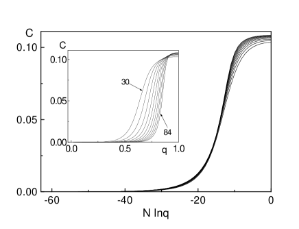
FIG. 2.: The correlation function $C=\langle A_{1}A_{N/2}\rangle$ as a function of the scaled variable $N{\ln}q$ for $N=30,36,42,\ldots,84$. The inset shows the same data plotted against $q$. Note that at $q=1$ the curves approach $1/9$ as $N$ increases (see text).

C. Discussion: The analysis presented above dealt with the case $N_{A}=N_{B}=N_{C}$. In the general case where the densities of the three species are not equal, detailed balance is not satisfied. However, the heuristic arguments for phase separation given at the beginning of the Letter are expected to hold for the general case provided that none of the densities is zero. Namely, configurations of the type $\ldots AAABBBBCCAAA\ldots$ are stable, and the time for a totally phase separated state to break up grows exponential in $N$. Numerical simulations of the model supports the existence of phase separation [10].

We thank D. Kandel, J. L. Lebowitz, S. Ramaswamy and E. R. Speer for interesting discussions. The support of Minerva Foundation, Munich, Germany (DM), The Royal Society and The Einstein Center (MRE) are gratefully acknowledged.

REFERENCES

- [1] S. Katz, J. L. Lebowitz, H. Spohn, Phys. Rev. B 28, 1655 (1983); J. Stat. Phys. 34, 497 (1984).
- [2] B. Schmittmann and R. K. P. Zia Statistical Mechanics of Driven Diffusive Systems in Phase Transitions and Critical Phenomena (C. Domb and J. L. Lebowitz, eds.) 17 (Academic Press, London, 1995).
- [3] T. Halpin-Healy and Y-C. Zhang, Phys. Rep. 254, 215 (1995).
- [4] M. R. Evans, D. P. Foster, C. Godrèche and D. Mukamel Phys. Rev. Lett. 74, 208 (1995); C. Godrèche et al, J. Phys. A 28, 6039 (1995).
- [5] P. Gacs, J. Comput. Sys. Sci. 32, 15 (1986).
- [6] S. A. Janowsky and J. L. Lebowitz, Phys. Rev. A 45, 618 (1992); B. Derrida, S. A. Janowsky, J. L. Lebowitz, E. R. Speer, Europhys. Lett. 22, 651 (1993); K. Mallick, J. Phys. A. 29, 5375 (1996).
- [7] R. Lahiri and S. Ramaswamy Cond-Mat 9610022.
- [8] A. J. Bray, Adv. Phys. 43, 357 (1994).
- [9] G. E. Andrews The Theory of Partitions, Encyclopedia of Mathematics and its Applications 2, p. 1–4 (Addison Wesley, MA, 1976).
- [10] M. R. Evans, Y. Kafri, H. M. Koduvely, and D. Mukamel, unpublished.
- [11] B. Derrida, M. R. Evans, V. Hakim and V. Pasquier, J. Phys. A 26, 1493 (1993).