Maxwell-Schrödinger Equation for Polarized Light and Evolution of the Stokes Parameters

Abstract

By starting with the Maxwell theory of electromagnetism, we study the change of polarization state of light transmitting through optically anisotropic media. The basic idea is to reduce the Maxwell equation to the Schrödinger like equation for two levels (or states) representing polarization. By using the quantum mechanical technique, the density matrix, and path integral, the evolution of the Stokes parameters results in the equation of motion for a pseudospin representing a point on the Poincaré sphere. Two typical examples relevant to actual experiments are considered; the one gives the generalized Faraday effect, and the other realizes an optical analog of magnetic resonance.

The study of propagation of light (or an electromagnetic wave) in optical media has long been one of the major subjects in physics. We mention, for example, the classic monographs [1, 2], and the works on nonlinear optics [3, 4]. The characteristic quantity describing the light propagation is the concept of polarization. The study of polarization has also a long history [1, 2], which forms a basis of modern crystal optics. The simple way to describe the polarization state is given by the Stokes parameters (or vector). Geometrically, the Stokes vector is realized as a point on the so-called Poincaré sphere. The Stokes vector or Poincaré sphere play a powerful role for analyzing the change of the polarization state of light transmitting through anisotropic optical media [2]. As for the equation for evolution of the Stokes parameters, the phenomenological description has been known in the area of optics, which uses special mathematical device such as the Jones vector or Müller matrix [5, 6, 7].

Having given a brief overview of the developments achieved so far, we address a novel formalism of the evolution for the polarization state of light transmitting through anisotropic media. Apart from the previous phenomenological approaches [5, 6, 7], our theory is based on the first principle starting from the Maxwell theory of electromagnetism [1], where we use the more refined form than the original Maxwell equation. Namely, the Maxwell equation is reduced to the wave equation á la Schrödinger equation for two levels [8], which is of first order in time (we call this the Maxwell-Schrödinger equation hereafter) and the dielectric tensor plays a role of Hamiltonian. By applying the technique used in usual quantum mechanics, such as density matrix as well as path integral, to the Maxwell-Schrödinger equation, we obtain the evolution equation for the Stokes parameters as an equation for a pseudospin which represents a point on the Poincaré sphere. This is our main consequence. As typical applications of the equation of motion for pseudospin, we consider the polarization change in specific media, for which the dielectric tensor has the same structure as the Hamiltonian for a real spin in external magnetic field. Specifically we are concerned with two cases: The first example is the pseudospin in uniform “magnetic field” which leads to the generalized Faraday effect. The second example is the pseudospin in oscillating as well as uniform field, by which we conjecture a possible occurrence of an optical analog of the nuclear magnetic resonance (NMR). These examples may be accessible to actual experiments and would enable us to reveal new aspects of polarization phenomena that have not been expected by previous works.

Maxwell-Schrödinger equation.—

We consider the plane electromagnetic (EM) wave of the wave vector $k$ ($k$ means the wave vector in the vacuum) travelling through the dielectric medium in the $z$ direction. The medium is anisotropic with respect to the propagation direction and let $\hat{\epsilon}$ be the dielectric tensor. We assume $z$ axis to be one of the principal axes of the dielectric tensor, namely, the direction along which the one of the eigenvalue of $\hat{\epsilon}$. When the medium is isotropic, the eigenvalue is prescribed to take the value $n_{0}$. Thus the EM wave has the form like $D(z,t)={\bf D}(z)\exp[i\omega t],$ and the wave equation for the displacement vector ${\bf D}(z)$ is given by [1]

$${d^{2}{\bf D}\over dz^{2}}+k^{2}\hat{\epsilon}{\bf D}=0,$$ (1)

where $k={\omega\over c}$. In the geometry under consideration, the dielectric tensor is taken to be $2\times 2$ matrix. Under the most general condition that is governed by the external static electric and magnetic fields or mechanical constraint, $\hat{\epsilon}$ can be chosen to be a Hermitian matrix [1], which means that the medium is transparent for the light transmission (we will consider elsewhere the case that there is an effect of absorption of light). Furthermore we consider the general situation that the medium is inhomogeneous, namely, the $\hat{\epsilon}$ depends on $z$. We now set the ansatz for the wave ${\bf D}$

$${\bf D}(z)={\bf f}(z)\exp[ikn_{0}z],$$ (2)

where the amplitude ${\bf f}(z)$ is given by the $2\times 1$ row vector,

$${\bf f}={}^{t}(f_{1},f_{2})=f_{1}{\bf e_{1}}+f_{2}{\bf e_{2}}.$$ (3)

f is a slowly varying function of $z$ compared with the wave length, namely, $k>>|f^{\prime}|$, which implies that we consider the short range approximation. Here $({\bf e}_{1},{\bf e}_{2})$ denotes the basis of linear polarization. In the short wave approximation, the amplitude is shown to satisfy the equation

$$i\lambda{d{\bf f}\over dz}+(\hat{\epsilon}-n_{0}^{2}){\bf f}=0,$$ (4)

where $\lambda\equiv{n_{0}\over k}$ is just the wave length in the medium of refractive index $n_{0}$ divided by $2\pi$. Note that the second order differential term $f^{\prime\prime}$ is discarded, since this is much smaller than the first order differential $f^{\prime}$. In this way, the above equation can be regarded as an analog of the Schrödinger equation for two-level state, where $\lambda$ just plays a role of the Planck constant and $z$ plays a role of the time variable. The components $(f_{1},f_{2})$ of the vector ${\bf f}$ couple each other to give rise to the change of polarization and the “Hamiltonian” is given by $\hat{h}=\hat{\epsilon}-n_{0}^{2}$. This form of $\hat{h}$ represents the deviation from the isotropic value, that is, “degree of anisotropy”, namely, the deviation governs the change of polarization state. From the hermiticity, the most general form of this is written as

$$\hat{h}=\left(\begin{array}[]{cc}\alpha&\beta+i\gamma\\ \beta-i\gamma&-\alpha\end{array}\right).$$ (5)

Now for the later use, it is convenient to transform the basis of linear polarization ${\bf f}$ into the circular basis [9], that is, ${\bf e_{\pm}}={1\over\sqrt{2}}({\bf e}_{1}\pm i{\bf e}_{2})$, hence the Schrödinger equation becomes

$$i\lambda{d\psi\over dz}=\hat{H}\psi,$$ (6)

where $\psi=T{\bf f}={}^{t}(\psi_{1}^{*},\psi_{2}^{*}),\;\hat{H}=T\hat{h}T^{-1}$. Here $T$ is the unitary transformation of the $2\times 2$ matrix given by

$$T={1\over\sqrt{2}}\left(\begin{array}[]{cc}1&i\\ 1&-i\end{array}\right).$$ (7)

Thus the transformed Hamiltonian turns out to be

$$\hat{H}=T\hat{h}T^{-1}=\left(\begin{array}[]{cc}\gamma&\alpha+i\beta\\ \alpha-i\beta&-\gamma\end{array}\right),$$ (10)

which is written in terms of the Pauli spin; $\hat{H}=\sum_{i=1}^{3}h_{i}\sigma_{i}$. The formal solution of the above Schrödinger equation is given by $\psi(z)=\hat{T}(z)\psi(0)$ with $\hat{T}(z)$ being the evolution operator,

$$\hat{T}(z)=P\exp[-{i\over\lambda}\int\hat{H}(z)dz].$$ (11)

Here $P$ denotes the path ordered product which is necessary to handle the $z$ dependence of $\hat{H}$.

Density matrix and equation of motion of the Stokes parameters.—

We now consider the reduction of the above Schrödinger equation. This is carried out by using the density matrix, for which we have two cases, the pure polarization and the mixed polarization (or partially polarized) state. Here we restrict ourselves to the former case in order to simplify the argument [10], thus the density matrix is defined as

$$\rho=\psi\psi^{\dagger}=\left(\begin{array}[]{cc}\psi_{1}^{*}\psi_{1}&\psi_{1}\psi_{2}^{*}\\ \psi_{2}\psi_{1}^{*}&\psi_{2}^{*}\psi_{2}\end{array}\right).$$ (12)

In terms of the components of the function $\psi$ given above, we have the definition for the Stokes parameter [11]; $S_{i}=\psi^{\dagger}\sigma_{i}\psi,S_{0}=\psi^{\dagger}1\psi$, where $\sigma_{i}(i=1,2,3)$ means the Pauli spin matrix. These variables satisfy the relation $S_{0}^{2}=S_{1}^{2}+S_{2}^{2}+S_{3}^{2}$, which is equivalent to the equation ${\rm det}\rho=0$. Furthermore, in the case that the Hamiltonian is Hermitian, we can adopt the conservation of probability $\psi_{1}^{*}\psi_{1}+\psi_{2}^{*}\psi_{2}=1$. So if we use the spinor parametrization

$$\psi_{1}=\cos{\theta\over 2},\quad\psi_{2}=\sin{\theta\over 2}\exp[i\phi],$$ (13)

we have $\rho={1\over 2}(1+{\bf S}{\bf\sigma})$, where the vector ${\bf S}=(S_{x},S_{y},S_{z})$ is given by

$$S_{x}=\sin\theta\cos\phi,\quad S_{y}=\sin\theta\sin\phi,\quad S_{z}=\cos\theta.$$ (14)

This forms the Stokes vector and is described by the point on the Poincaré sphere. We illustrate some typical values: (i) $\theta=0$; the north pole that corresponds to the left handed circular polarization. (ii) $\theta=\pi$; the south pole that corresponds to the right handed circular polarization. (iii) $\theta={\pi\over 2}$; the equator which represents the linear polarization. The equation of motion for the density matrix is written as

$$i\lambda{d\rho\over dz}=[\hat{H},\rho].$$ (15)

Here $[\hat{H},\rho]\equiv\hat{H}\rho-\rho\hat{H}$. Using the commutation relation for the Pauli spin, $[\sigma_{i},\sigma_{j}]=2i\epsilon_{ijk}\sigma_{k}$, we can deduce the equation of motion for the pseudospin from (15)

$$\lambda{d{\bf S}\over dz}={\bf S}\times{\bf G},$$ (16)

where the effective “magnetic field” is defined as ${\bf G}=(2\alpha,2\beta,2\gamma)$. If we introduce the “classical” counterpart of the Hamiltonian (10)

$$H = 2\alpha S_{x}+2\beta S_{y}+2\gamma S_{z}\quad$$ (17)

$$= 2\alpha\sin\theta\cos\phi+2\beta\sin\theta\sin\phi+2\gamma\cos\theta,$$ (18)

we have an alternative form of the equation of motion [12]

$$\dot{\theta}={1\over\lambda\sin\theta}{\partial H\over\partial\phi},\quad\dot{\phi}=-{1\over\lambda\sin\theta}{\partial H\over\partial\theta}.$$ (19)

The equation of motion (19) can also be obtained as a result of the asymptotic limit of $\lambda\rightarrow 0$ [13]. This may be achieved by the fact that the set of states for pseudospin, ${\psi\equiv|\psi>}$ forms a Bloch state that satisfies the completeness relation: $\int|\psi>d\mu<\psi|=1$ with measure $d\mu=\sin\theta d\theta d\phi$ (just the volume on the Poincaré sphere). Let us consider the transition amplitude that is given by sandwiching the evolution operator (11) with two initial and final spin states. By adopting the procedure of “time slicing” and inserting the completeness relation at each time division, we get the path integral expression [14]

$$<\psi_{f}|\hat{T}(z)|\psi_{i}>=\int\exp\left\{{i\over\lambda}S[\psi^{*},\psi]\right\}D\mu(\psi)$$ (20)

with the path measure $D\mu(\psi)\equiv\prod_{z}d\mu[\psi^{*}(z),\psi(z)]$ and $S$ is the “action function”

$$S=\int<\psi|i\lambda{d\over dz}-\hat{H}|\psi>dz.$$ (21)

In the limit of $\lambda\rightarrow 0$, we have the stationary phase condition $\delta S=0$ leading to the equation of motion for the pseudospin, i.e., (19).

Typical applications.—

We shall consider some special cases that can be described by the general formalism. (i) We first consider the model for which the dielectric tensor depends on the external magnetic field as well as electric field. The kinematical symmetry implies that $\hat{h}$ has the form

$$\hat{h}=\left(\begin{array}[]{cc}\alpha&i\gamma\\ -i\gamma&-\alpha\\ \end{array}\right).$$ (22)

Here $\gamma$ is proportional to the uniform magnetic field (the strength is ${\bf B}$) applied in the $z$ direction; $\gamma={\rm g}B$ [15]. Thus according to the formula (10), it is transformed to $\hat{H}=\gamma\sigma_{z}+\alpha\sigma_{x}$. This is further transformed to the Hamiltonian for the spin in uniform field of strength $\Gamma$, that is applied in the $z^{\prime}$ direction by rotating about the $y$ axis by an amount of the angle $\eta$, such that

$$S_{x}^{\prime}=\cos\eta S_{x}-\sin\eta S_{z},\quad S_{z}^{\prime}=\sin\eta S_{x}+\cos\eta S_{z},$$ (23)

where $\Gamma=\sqrt{\gamma^{2}+\alpha^{2}}$ together with the angle $\cos\eta=\gamma/\Gamma$. Thus the equation of motion for the pseudospin becomes

$${dS_{x}^{\prime}\over dz}={2\Gamma\over\lambda}S_{y},\quad{dS_{y}\over dz}=-{2\Gamma\over\lambda}S_{x}^{\prime}$$ (24)

for which we get the solution $S_{x}^{\prime}=\sin({2\Gamma\over\lambda}z+\theta_{0}),\,S_{y}=\cos({2\Gamma\over\lambda}z+\theta_{0})$ and $S_{z}^{\prime}=0$. In terms of the original spin, it gives

$$S_{x}=\cos\eta\sin({2\Gamma\over\lambda}z+\theta_{0}),\quad S_{z}=-\sin\eta\sin({2\Gamma\over\lambda}z+\theta_{0}).$$ (25)

This means the following feature, if the light wave is initially in the linear polarization, then it turns out to be an elliptic polarization after transmitting through the medium (see Fig. 2). As a special case of $\alpha=0$, the initial polarization changes to $S_{x}=\sin({2\gamma\over\lambda}z+\theta_{0}),\;S_{y}=\cos({2\gamma\over\lambda}z+\theta_{0})$, namely, the initial polarization plane simply changes by an amount of the angle $\phi={2\gamma\over\lambda}l$ after travelling the distance $z=l$. This rotation of the polarization plane is known to be the Faraday effect [see Fig. 2(a)].

(ii) We consider another example for which the polarized light propagates in the medium such that the dielectric tensor has a periodical structure besides the effect of the external magnetic field as in the case (i). For such a system the tensor $\hat{h}$ is given by

$$\hat{h}=\left(\begin{array}[]{cc}\gamma_{0}\cos\omega z&\gamma_{0}\sin\omega z\\ \gamma_{0}\sin\omega z&-\gamma_{0}\cos\omega z\end{array}\right)+\left(\begin{array}[]{cc}0&i\gamma\\ -i\gamma&0\end{array}\right),$$ (26)

which is transformed to $\hat{H}(z)={\bf G}(z){\bullet}{\bf S}$, where the pseudomagnetic field has the component:

$${\bf G}(z)=(2\gamma_{0}\cos\omega z,\;2\gamma_{0}\sin\omega z,\;2\gamma),$$ (27)

namely, a static field along the $z$ axis plus an oscillating field rotating perpendicular to it with the frequency $\omega$. This feature is familiar in magnetic resonance. Using the classical counterpart of the above Hamiltonian, which is given as $H(z)={\bf G}(z)\cdot{\bf S}=2\gamma_{0}\sin\theta\cos(\phi-\omega z)+2\gamma\cos\theta$, the equation of motion is derived by using the general formula (19)

$$\dot{\theta} = -{2\gamma_{0}\over\lambda}\sin(\phi-\omega z),$$ (28)

$$\dot{\phi} = -{2\over\lambda}[\gamma_{0}\cot\theta\cos(\phi-\omega z)-\gamma].$$ (29)

One sees that this form of equations of motion allows a special solution

$$\phi=\omega z,\quad\theta=\theta_{0}(={\rm const}),$$ (30)

where the following relation should hold among the parameters $\theta_{0},\gamma,\gamma_{0}$:

$$\cot\theta_{0}=\left({\gamma\over\gamma_{0}}-{{\lambda\omega}\over 2\gamma_{0}}\right).$$ (31)

Equation (30) may be called the “resonance” solution, since it corresponds to the solution for the forced oscillator. The set of parameters $(\gamma,\gamma_{0},\omega)$ satisfying (31) for a fixed value $\theta=\theta_{0}$ belong to a family of resonance solutions. Indeed, this set of parameters forms a surface in the parameter space $(\gamma,\gamma_{0},\omega)$, which we call the “invariant surface” and characterizes the resonance condition. The condition (31) is crucial, since all the quantities on the right hand side are given in terms of constants that may be allowed to be compared with experiment. The physical meaning of the above invariant surface is as follows: If given is an initial elliptic polarized wave with the angle $\theta_{0}$ satisfying the resonance condition, then there is no change in its shape during its transmission. Only its axis rotates by an amount of $\omega l$ that is governed by the period inherent in the dielectric tensor [see Fig. 2(b)].

Here we give a remark on possible realization of the periodic structure of the dielectric tensor in actual systems. The one realization is made by using special materials, such as cholesteric liquid crystals [16]. The periodic structure is naturally realized by the helix inherent in liquid crystal. Indeed, the dielectric tensor can be given by the form of the first term of (26) [16]. Another realization may be given by using the mechanical one, namely, let us consider the elastic body under the pressure that is periodically modulated, then this causes the periodic modulation of the dielectric tensor according to the procedure known in the mechanical-optical effect [1]. The periodical oscillation of the pressure may be generated, for example, by the piezoelectric effect. Now having settled the periodic structure, we take into account the term coming from the uniform magnetic field that is applied along the same direction as the axis of helix. We are reminded of the analogy with the NMR; if the initial state is in the left handed circular polarization, which corresponds to the state of spin-down, the probability for transition to the state of spin-up (right handed circular polarization) is given by

$$P(l\rightarrow r)={(\gamma_{0}^{\prime})^{2}\over(\Omega-\omega)^{2}+(\gamma_{0}^{\prime})^{2}}\sin^{2}{1\over 2}\Delta z,$$ (32)

where $\gamma_{0}^{\prime}\equiv{\gamma_{0}\over\lambda}$ and $\Omega={\gamma\over\lambda}$ and $\Delta^{2}=(\Omega-\omega)^{2}+(\gamma_{0}^{\prime})^{2}$. If the magnetic field is chosen so as to synchronize the period of the helix, we expect an analogous effect with the magnetic resonance.

This work was inspired by the discussion at seminar class that had been instructed by one of the authors (H.K.). The authors thank the attendees of the seminar.

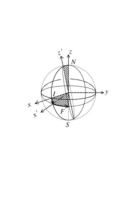
FIG. 1.: The initial linear polarization, which is marked by $I$, changes to the final elliptic polarization are marked by $F$.

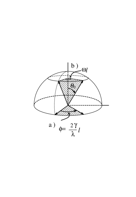
FIG. 2.: (a) The change of linear polarization by an amount of $\phi={2\gamma\over\lambda}l$,   (b) The change of the axis of elliptic polarization by an amount of $\omega l$.

REFERENCES

- [1] L. Landau and E. Lifschitz, Electrodynamics in Continuous Media, Course of Theoretical Physics Vol.8 (Pergamon Oxford, 1968).
- [2] M. Born and E. Wolf, Principle of Optics (Pergamon, Oxford, 1975).
- [3] R. Y. Chiao, E. Gamire, and C. H. Townes, Phys. Rev. Lett. 13, 479 (1964).
- [4] G. A. Swartzlander, Jr. and C. T. Law, Phys. Rev. Lett. 69, 2503 (1992), and references therein.
- [5] R. Azzam, J. Opt. Soc. Am. 68, 1756 (1978).
- [6] C. Brosseau, Opt. Lett. 20, 1221 (1995), and references therein.
- [7] R. C. Jones, J. Opt. Soc. Am. 38, 671 (1948).
- [8] The similar reduction has been previously obtained by Chiao et al.: R. Chiao and J. Goldine, Phys. Rev. 185, 430 (1969), which deals with the nonlinear Schrödinger equation and does not take into account the anisotropic effect.
- [9] J. J. Sakurai, Advanced Quantum Mechanics (Wiley, New York, 1967).
- [10] To consider the partially polarized state means that one should treat the time-varying function of the polarization. This implies that the polarization is distributed over a certain range of frequency, which is denoted by some parameter . Thus we treat the partially polarized state by using the statistical distribution , . (Note that the wave function is also paramtetrized by the parameter ). See L. Landau and E. Lifschitz, Classical Fields, Course of Theoretical Physics Vol.5 (Pergamon, Oxford, 1968).
- [11] G. C. Wick, in Prelude in Theoretical Physics, edited by A. deShalit, H. Feshbach, and L. van Hove (North-Holland Publishing, Amsterdam, 1966).
- [12] see e.g., F. A. Berezin, Commum. Math. Phys. 40, 153 (1975).
- [13] The procedure given below is also applicable for the case of nonlinear media, for which the dielectric tensor is given in terms of the quadratic form of the pseudospin.
- [14] H. Kuratsuji and T. Suzuki, J. Math. Phys. (N.Y.) 21, 419 (1980).
- [15] It is known [1] that the dielectric tensor has the form with in the case that only the magnetic field is applied in the direction of light propagation.
- [16] P. de Gennes, Physics of Liquid Crystal (Oxford University Press, Oxford, 1993), 2nd ed.