A coherent double-quantum-dot electron pump

A quantum dot can be thought of as an artificial atom with adjustable parameters. It is of more than fundamental interest to study its properties under various circumstances, e.g. by transport experiments[1]. By considering a double-quantum-dot system, the analogy with real atoms can be stretched to include artificial molecules. The analogue of the covalent bond is then formed by an electron which coherently tunnels back and forth between the two dots. By applying electromagnetic radiation with a frequency equal to the energy difference between the time-independent eigenstates of the double-dot system, an electron can undergo these so-called spatial Rabi oscillations even when the tunneling matrix element between the dots is small [2, 3]. Recently, several time-dependent transport measurements on quantum-dot systems have been reported [4], most of them aimed to characterize the discrete states in the dots. It has also been suggested to make devices from quantum dots. Examples of such applications are pumps that transfer electrons one by one by using time-dependent voltages to alternatingly raise and lower tunnel barrier heights [5], or systems in which coupled quantum dots (or quantum wells) are used for quantum-scale information processing [6]. Because the transport mechanism in the abovementioned pumps is determined by sequential tunneling, electrons are pumped incoherently. In this paper we describe an electron pump that can also transfer electrons coherently by means of a co-tunneling process. In this case, the system switches coherently between two states each time an electron is pumped through the dots. The number of electrons in the double dot does not change, however, resulting in less current noise. Alternatively, this process can be seen as coherent transport through a double-quantum-dot qubit.

The system we consider consists of two weakly coupled quantum dots A and B connected to two large reservoirs L and R by tunnel barriers (see Fig. 1).

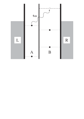
FIG. 1.: Asymmetric double-dot system at zero bias voltage. The dots A and B are coupled to the reservoirs L and R by tunnel junctions. An electron in the left dot can tunnel to the right by absorbing a photon.

The leads are assumed to have a continuous energy spectrum and the bias voltage is zero. Each individual quantum dot is in its ground state and in the remainder of this paper we will only concentrate on the case of transitions between ground states of the dots. Moreover, we assume that the double-dot system is asymmetric in the ground state $|0,0\rangle$, where $|n,m\rangle$ denotes a full many-body state with $n$ extra electrons in the left dot and $m$ in the right dot, respectively. This asymmetry entails that the energy of the state $|1,-1\rangle$ is much higher than the energy of the state $|-1,1\rangle$. In that case an electron can be excited from the left dot into the right one, but the probability of the reverse process occurring can be neglected. By fabricating two dots of different sizes and adjusting the energy levels with a gate voltage, such an asymmetry can be easily realized. The energy difference between the ground state $|{a}\rangle=|0,0\rangle$ and the excited state $|{b}\rangle=|-1,1\rangle$ is denoted by $\varepsilon_{0}$. It can be tuned by an external gate voltage, and we assume it to be much larger than the transition matrix element between the dots $T$, i.e. $\varepsilon_{0}\gg T$. In this case dc transport through the double dot is blocked.

This situation changes if we apply electromagnetic radiation to the system. Assume that a time-dependent oscillating signal is present on the gate electrode, so that the time-dependent energy difference between states $|{a}\rangle$ and $|{b}\rangle$ becomes $\varepsilon(t)=\varepsilon_{0}+\tilde{\varepsilon}\cos\omega t$, where $\tilde{\varepsilon}$ is the amplitude and $\omega$ the frequency of the externally applied signal. When the frequency of the applied radiation matches the time-independent energy difference between states $|{a}\rangle$ and $|{b}\rangle$, i.e. if $\omega\approx\varepsilon_{0}$, it is possible for an electron from the left dot to tunnel to the right one. In principle, this electron can now leave the system by tunneling to the right lead, resulting in state $|{c}\rangle=|-1,0\rangle$. An electron from the left lead can then tunnel to the left dot, thus restoring the ground state. Effectively, an electron has now been transferred from the left electrode to the right one. This transport cycle, $|0,0\rangle\rightarrow|-1,1\rangle\rightarrow|-1,0\rangle\rightarrow|0,0\rangle$, is not the only one. Another possible sequence, in which the system passes the intermediate state $|{d}\rangle=|0,1\rangle$, is given by $|0,0\rangle\rightarrow|-1,1\rangle\rightarrow|0,1\rangle\rightarrow|0,0\rangle$.

The details of the transport mechanism of a pumping cycle depend on the energies of states $|{c}\rangle$ and $|{d}\rangle$, as shown in Fig. 2.

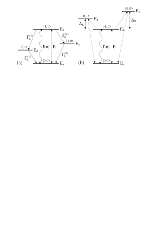
FIG. 2.: Energy diagrams of the double-dot system in which (a) only incoherent and (b) only coherent tunneling occurs. Indicated are the four possible states of the system and their respective energies: $|{a}\rangle=|0,0\rangle$, $|{b}\rangle=|-1,1\rangle$, $|{c}\rangle=|-1,0\rangle$, and $|{d}\rangle=|0,1\rangle$.

If the energies of these intermediate states are somewhere between those of states $|{a}\rangle$ and $|{b}\rangle$, the double-dot system relaxes to the ground state via the sequential (and thus incoherent) tunneling processes described above. As shown in Fig. 2 (a), the four tunneling processes are described by the rates $\Gamma_{L}^{(1)}$, $\Gamma_{R}^{(1)}$, $\Gamma_{L}^{(2)}$, and $\Gamma_{R}^{(2)}$, respectively. Here, units are used such that $\hbar=1$. In the opposite case when the energies of the intermediate states are higher than that of state $|{b}\rangle$, Fig. 2 (b), transport via sequential tunneling is blocked. However, transport is still possible via inelastic co-tunneling of electrons [7]. When the system is in state $|{b}\rangle$, two electrons can tunnel simultaneously, one going from the left reservoir to the left dot and the other going from the right dot to the right electrode. In this process one of the intermediate states is virtually occupied. The necessary energy is provided by relaxing the system to the ground state $|a\rangle$, thereby releasing an energy $E$. In the following, we will describe these two different mechanisms quantitatively, starting with the sequential tunneling regime.

We use the density-matrix approach developed in Ref. [9]. Disregarding tunneling to and from the leads, the Hamiltonian of the two-level system is given by:

$$\cal{H}=\left(\begin{array}[]{cc}-\frac{1}{2}(\epsilon_{0}+\tilde{\epsilon}\cos\omega t)&T\\ T&\frac{1}{2}(\epsilon_{0}+\tilde{\epsilon}\cos\omega t)\end{array}\right),$$ (1)

where $T$ describes the coupling between the dots. We are interested in the particular case where the energy level spacing is large, i.e. $\epsilon_{0}\gg T$. Rewriting Eq. (1) in the basis of eigenstates of the time-independent ($\tilde{\epsilon}=0$) Hamiltonian and using the fact that $\tilde{\epsilon}\ll\epsilon_{0}$, we obtain:

$$\cal{H}=\left(\begin{array}[]{cc}-\frac{1}{2}E&\overline{T}\cos\omega t\\ \overline{T}\cos\omega t&\frac{1}{2}E\end{array}\right),$$ (2)

where $E=\sqrt{\epsilon_{0}^{2}+4T^{2}}\approx\epsilon_{0}$ is the renormalized energy level spacing and $\overline{T}=T\tilde{\epsilon}/E$. From Eq. (2) we see that there are small time-dependent matrix elements that cause mixing between the two states. Using the equation of motion for the density matrix, $id\rho/dt=[\cal{H},\rho]$, including tunneling to and from the leads, and disregarding rapidly oscillating terms, we obtain the equations of motion for the density-matrix elements which are valid near resonance:

$$\dot{\rho}_{aa} = +i\mbox{$\frac{1}{2}$}\overline{T}(\rho_{ab}-\rho_{ba})+\Gamma_{L}^{(2)}\rho_{cc}+\Gamma_{R}^{(1)}\rho_{dd},$$ (4)

$$\dot{\rho}_{bb} = -i\mbox{$\frac{1}{2}$}\overline{T}(\rho_{ab}-\rho_{ba})-\Gamma_{T}\rho_{bb},$$ (5)

$$\dot{\rho}_{cc} = \Gamma_{R}^{(2)}\;\rho_{bb}-\Gamma_{L}^{(2)}\;\rho_{cc},$$ (6)

$$\dot{\rho}_{ab} = i\mbox{$\frac{1}{2}$}\overline{T}(\rho_{aa}-\rho_{bb})+i(E-\omega)\rho_{ab}-\mbox{$\frac{1}{2}$}\Gamma_{T}\rho_{ab},$$ (7)

where $\Gamma_{T}=\Gamma_{L}^{(1)}+\Gamma_{R}^{(2)}$ and $\rho_{aa}$, $\rho_{bb}$, $\rho_{cc}$, and $\rho_{dd}=1-\rho_{aa}-\rho_{bb}-\rho_{cc}$ denote the probabilities for an electron to be in the states $|{a}\rangle$, $|{b}\rangle$, $|{c}\rangle$ and $|{d}\rangle$, respectively. In the nondiagonal elements $\rho_{ab}=\rho_{ba}^{*}$, only the frequency parts $\rho_{ab}\exp(i\omega t)$ and $\rho_{ba}\exp(-i\omega t)$ that contribute to the resonant current peak have been retained.

The average current through the system is given by:

$$I/e=\Gamma_{R}^{(2)}\rho_{bb}+\Gamma_{R}^{(1)}\rho_{dd}.$$ (8)

In Fig. 3 we have plotted a resonant current peak

FIG. 3.: The pumping current as a function of the applied frequency for different values of $\Gamma/\overline{T}$, where we have taken $\Gamma_{L}^{(1)}=\Gamma_{R}^{(1)}=\Gamma_{L}^{(2)}=\Gamma_{R}^{(2)}=\Gamma$. Calculated for $\tilde{\varepsilon}=0.1\varepsilon_{0}$ and $T=0.1\varepsilon_{0}$.

as a function of the applied radiation frequency for different values of $\Gamma/\overline{T}$, where $\Gamma=\Gamma_{L}^{(1)}=\Gamma_{R}^{(1)}=\Gamma_{L}^{(2)}=\Gamma_{R}^{(2)}$. The current peak height initially grows with increasing $\Gamma$, its width remaining almost constant. The best resonance condition occurs for $\Gamma=\overline{T}$. When $\Gamma$ increases beyond this value, the height of the peak rapidly decreases while the width increases. Using an approach developed in Ref. [2], which is valid near resonance, we are able to derive an analytical expression for the shape of the current peak in this regime. We find that the peak is a Lorentzian:

$$I/e = I_{max}w^{2}/[w^{2}+4(\omega-E)^{2}],$$ (10)

$$I_{max} = \overline{T}^{2}\Gamma_{T}/[\Gamma_{T}^{2}+(2+\alpha)\overline{T}^{2}],$$ (11)

$$w = \sqrt{\Gamma_{T}^{2}+(2+\alpha)\overline{T}^{2}},$$ (12)

where $\alpha=\Gamma_{L}^{(1)}/\Gamma_{R}^{(1)}+\Gamma_{R}^{(2)}/\Gamma_{L}^{(2)}$. In the limit of small $\overline{T}$, i.e. in the limit of small radiation amplitude $\tilde{\varepsilon}$ and small overlap $T$, the height of the current peak is proportional to $\overline{T}^{2}$; $I_{max}=\overline{T}^{2}/\Gamma_{T}$, whereas its width is constant in this limit; $w=\Gamma_{T}$. This concludes the discussion of the incoherent tunneling regime.

In the coherent mechanism, two electrons tunnel simultaneously; one going from the left lead to the left dot, and one from the right dot to the right lead. Because the transport occurs via the virtual occupation of a state with a large electrostatic energy, these two tunneling events cannot be treated independently[7]. Using Fermi’s Golden Rule we obtain the zero-temperature co-tunnel rate[8]:

$$\Gamma_{ct} = \frac{2C\left[\ln(1+E/\Delta_{L})+\ln(1+E/\Delta_{R})\right]}{\Delta_{L}+\Delta_{R}+E}+$$ (14)

$$\frac{CE}{\Delta_{L}\left(\Delta_{L}+E\right)}+\frac{CE}{\Delta_{R}\left(\Delta_{R}+E\right)},$$

where $C=2\pi|t_{L}t_{R}|^{2}\nu_{L}\nu_{R}$, and where the matrix elements for tunneling trough the left and right barier, $t_{L,R}$, and the density of states in the left and right electrode, $\nu_{L,R}$, are assumed to be energy independent. In the limit of large charging energies, $\Delta_{L},\Delta_{R}\gg E$, which we will consider from now on, Eq. (14) reduces to a simple expression:

$$\Gamma_{ct}=2\pi|t_{L}t_{R}|^{2}\nu_{L}\nu_{R}\left(\frac{1}{\Delta_{L}}+\frac{1}{\Delta_{R}}\right)^{2}E.$$ (15)

The prefactor $C$ is proportional to the product of the individual tunnel rates through the left and right barrier, and the energy denominators reflect the fact that the tunneling occurs via the virtual occupation of two states. Because co-tunneling is a second-order process, this co-tunnel rate will be much smaller than the sequential tunnel rates of the incoherent regime. In the absence of radiation, the average current through the system is given by:

$$I/e=\Gamma_{ct}\rho_{bb},$$ (16)

which is zero, since $\rho_{bb}=0$. In order to calculate the current in the presence of radiation, we therefore need equations for the density matrix elements $\rho_{aa}$ and $\rho_{bb}$ taking into account the radiation-induced co-tunneling processes. In contrast to the situation in the incoherent mechanism, these density matrix elements are the only diagonal ones because the states $|{c}\rangle$ and $|{d}\rangle$ are now occupied only virtually.

As before, we choose the eigenstates of the time-independent Hamiltonian as the basis for our calculations. The time-dependent Schrödinger equation then becomes:

$$id\vec{\psi}_{\alpha}(t)/dt={\cal H}(t)\vec{\psi}_{\alpha}(t),$$ (17)

where ${\cal H}$ is given by Eq. (2) and $\alpha=a,b$. Expanding the wave functions $\psi_{\alpha}(t)$ in harmonics we obtain:

$$\vec{\psi}_{\alpha}(t)=e^{-iE_{\alpha}t}\sum_{n}\vec{c}^{n}_{\alpha}e^{-in\omega t}.$$ (18)

In the case of a small radiation amplitude, $\tilde{\varepsilon}\ll\varepsilon_{0}$, and near resonance, $\omega\approx E$, it is a good approximation to retain only the $n=0$ and $n=1$ terms for $\vec{\psi}_{a}(t)$, and the $n=0$ and $n=-1$ terms for $\vec{\psi}_{b}(t)$. This approximation entails that we only take into account single-photon transitions between the states $|{a}\rangle$ and $|{b}\rangle$. The wave functions then become:

$$\vec{\psi}_{a}(t) = e^{-iE_{a}t}~{}(\xi\vec{\psi_{a}}-\zeta e^{-i\omega t}\vec{\psi_{b}}),$$ (20)

$$\vec{\psi}_{b}(t) = e^{iE_{a}t}~{}(\zeta e^{i\omega t}\vec{\psi_{a}}+\xi\vec{\psi_{b}}),$$ (21)

where the coefficients $\xi$ and $\zeta$ are given by:

$$\xi = (\delta E+W)/\sqrt{2W(W+\delta E)},$$ (23)

$$\zeta = \overline{T}/\sqrt{2W(W+\delta E)},$$ (24)

where $\delta E=E-\omega$ and $W^{2}={\delta E}^{2}+\overline{T}^{2}$. At resonance, when $\omega=E$, the coefficients are $\xi=\zeta=\frac{1}{2}\sqrt{2}$. The energy $E_{a}$ in Eqs. (20) and (21) is given by:

$$E_{a}=-E_{b}=-\mbox{$\frac{1}{2}$}E-\mbox{$\frac{1}{2}$}W,$$ (25)

reflecting the fact that the energy levels $-\frac{1}{2}E$ and $\frac{1}{2}E-\omega$ slightly repel each other when $\omega\approx E$.

With the aid of the closed-time-path Green function technique [10], which was applied to quantum-dot systems in Ref. [11], the wave functions Eqs. (20) and (21) are used to obtain the equations of motion for the density-matrix elements near resonance. Without going into the details of this calculation (they can be found in Ref. [8]), we simply present here the resulting set of equations:

$$\dot{\rho}_{bb} = -i\mbox{$\frac{1}{2}$}\overline{T}(\rho_{ab}-\rho_{ba})-\Gamma_{ct}\rho_{bb}+\xi^{2}\zeta^{2}\Gamma_{ct},$$ (27)

$$\dot{\rho}_{ab} = i\mbox{$\frac{1}{2}$}\overline{T}(\rho_{aa}-\rho_{bb})+i(E-\omega)\rho_{ab}-\mbox{$\frac{1}{2}$}\Gamma_{ct}\rho_{ab},$$ (28)

where $\rho_{aa}+\rho_{bb}=1$, $\rho_{ba}=\rho_{ab}^{*}$, and where we have used $\omega\approx E$ and $E_{a}\approx-E/2$ to calculate the dissipative terms. Clearly these equations are very similar to Eqs. (5) and (7). The crucial difference with the equations for the density matrix in the incoherent mechanism, however, is that the extra tunnel rate in Eq. (27) depends on the applied frequency and radiation amplitude via $\xi$ and $\zeta$: It is a Lorentzian centered around $\omega=E$ having width $2\overline{T}$.

We solve for the stationary solution of these equations to calculate the average current through the system which is given by the probability $\rho_{bb}$ to be in the excited state $|b\rangle$ times the decay rate of that state:

$$I/e=(\xi^{4}+\xi^{2}\zeta^{2}+\zeta^{4})\Gamma_{ct}\rho_{bb}.$$ (29)

In Fig. 4 the scaled pumping current is plotted for different values of $\Gamma_{ct}/\overline{T}$.

FIG. 4.: The scaled pumping current in the coherent regime as a function of the applied frequency for different values of $\Gamma_{ct}/\overline{T}$. Calculated for $\tilde{\varepsilon}=0.1\varepsilon_{0}$ and $T=0.1\varepsilon_{0}$.

With increasing co-tunnel rate, the scaled peak height first drops rapidly and then decreases slowly to its minimum value, while its width changes only slightly. The peak shape is a Lorentzian of the form Eq. (10) with height $I_{max}$ and width $w$:

$$I_{max} = \mbox{$\frac{3}{16}\Gamma_{ct}$}(4\overline{T}^{2}+\Gamma_{ct}^{2})/(2\overline{T}^{2}+\Gamma_{ct}^{2}),$$ (31)

$$w = \overline{T}\sqrt{6(2\overline{T}^{2}+\Gamma_{ct}^{2})(4\overline{T}^{2}+\Gamma_{ct}^{2})/(8\overline{T}^{4}+\Gamma_{ct}^{4}}).$$ (32)

The height $I_{max}$ reduces to $\frac{3}{8}\Gamma_{ct}$ for small $\Gamma_{ct}$ and to $\frac{3}{16}\Gamma_{ct}$ for large $\Gamma_{ct}$. A comparison with Fig. 3 clearly shows that the co-tunnel current peak is much narrower than the incoherent one. Another distinct feature of this co-tunnel peak is the fact that its width changes nonmonotonically with increasing co-tunnel rate $\Gamma_{ct}$. For small values of $\Gamma_{ct}$ the width is equal to $w=\sqrt{6}~{}\overline{T}\approx 2.45~{}\overline{T}$. It then increases rapidly to reach a maximum of $w=\sqrt{6+\frac{9}{2}\sqrt{2}}~{}\overline{T}\approx 3.52~{}\overline{T}$ for $\Gamma_{ct}=2^{3/4}~{}\overline{T}\approx 1.68~{}\overline{T}$. On increasing the co-tunnel rate further, the width decreases again to $\sqrt{6}~{}\overline{T}$. The width is thus comparatively insensitive to changes in the co-tunnel rate. This is due to the fact that the extra co-tunnel rate in Eq. (27) itself has an intrinsic width $w=2\overline{T}$, thus restricting the width of the current peak dramatically.

In conclusion, we considered an electron pump consisting of a double quantum dot subject to radiation. An incoherent and a coherent pumping mechanism has been discussed. By deriving equations of motion for the density matrix elements of the double-dot system, we calculated the pumping current in both regimes. Whereas the tunnel rates as a function of the external frequency are constants in the incoherent mechanism, they are Lorentzians in the co-tunneling regime. In both cases the current peak is a Lorentzian, but in the coherent case the peak width is much smaller than in the sequential-tunneling regime and changes nonmonotonically as a function of the co-tunnel rate. Experimental realization of this device would allow for a systematic study of coherent transport through a solid-state qubit.

It is a pleasure to acknowledge useful discussions with Gerrit Bauer, Henk Stoof, Caspar van der Wal, Tjerk Oosterkamp, and Leo Kouwenhoven. This work is part of the research program of the ”Stichting voor Fundamenteel Onderzoek der Materie” (FOM), which is financially supported by the ”Nederlandse Organisatie voor Wetenschappelijk Onderzoek” (NWO).

REFERENCES

- [1] L. P. Kouwenhoven and P. L. McEuen, in Nano-Science and Technology, edited by G. Timp, (AIP Press, New York 1996) and references therein.
- [2] T. H. Stoof and Yu. V. Nazarov, Phys. Rev. B 53, 1050 (1996).
- [3] C. A. Stafford and N. S. Wingreen, Phys. Rev. Lett. 76, 1916 (1996).
- [4] L. P. Kouwenhoven et al., Phys. Rev. B 50, 2019 (1994); L. P. Kouwenhoven et al., Phys. Rev. Lett. 73, 3443 (1994); Y. Nakamura et al., preprint; T. H. Oosterkamp et al., Phys. Rev. Lett. 78, 1536 (1997); T. Fujisawa and S. Tarucha, preprint.
- [5] L. P. Kouwenhoven et al., Phys. Rev. Lett. 67, 1626 (1991); F. W. J. Hekking and Yu. V. Nazarov, Phys. Rev. B 44, 9110 (1991).
- [6] R. Landauer, Science 272, 1914 (1996); A. Barenco, et al., Phys. Rev. Lett. 74, 4083 (1995); D. Loss and D. P. DiVicenzo, preprint.
- [7] D. V. Averin and A. A. Odintsov, Phys. Lett. A 140, 251 (1989); D. V. Averin and Yu. V. Nazarov, Phys. Rev. Lett. 65, 2446 (1990).
- [8] T. H. Stoof, Ph.D. thesis, Delft Univerity of Technology (1997), available upon request.
- [9] Yu. V. Nazarov, Physica B 189, 57 (1993); S. A. Gurvitz and Y. S. Prager, Phys. Rev. B 53, 15932 (1996).
- [10] See e.g. J. Rammer, Rev. Mod. Phys. 63, 781 (1991); H. Kleinert, Path Integrals in Quantum Mechanics, Statistics, and Polymer Physics (World Scientific, Singapore 1995).
- [11] H. Schoeller and G. Schön, Phys. Rev. B 50, 18436 (1994); J. König et al., Phys. Rev B 54, 16820 (1996); J. König et al., Phys. Rev. Lett. 78, 4482 (1997).