Random Matrix Theories in Quantum Physics: Common Concepts

Abstract

We review the development of random–matrix theory (RMT) during the last decade. We emphasize both the theoretical aspects, and the application of the theory to a number of fields. These comprise chaotic and disordered systems, the localization problem, many–body quantum systems, the Calogero–Sutherland model, chiral symmetry breaking in QCD, and quantum gravity in two dimensions. The review is preceded by a brief historical survey of the developments of RMT and of localization theory since their inception. We emphasize the concepts common to the above–mentioned fields as well as the great diversity of RMT. In view of the universality of RMT, we suggest that the current development signals the emergence of a new “statistical mechanics”: Stochasticity and general symmetry requirements lead to universal laws not based on dynamical principles.

MPI preprint H V27 1997, submitted to Physics Reports

Contents

toc

I Introduction

During the last ten years, Random Matrix Theory (RMT) underwent an unexpected and rapid development: RMT has been successfully applied to an ever increasing variety of physical problems.

Originally, RMT was designed by Wigner to deal with the statistics of eigenvalues and eigenfunctions of complex many–body quantum systems. In this domain, RMT has been successfully applied to the description of spectral fluctuation properties of atomic nuclei, of complex atoms, and of complex molecules. The statistical fluctuations of scattering processes on such systems were also investigated. We demonstrate these statements in Figs. 1, 2 and 3, using examples taken from nuclear physics. The histogram in Fig. 1 [1] shows the distribution of spacings of nuclear levels versus the variable $s$, the actual spacing in units of the mean level spacing $D$. The data set comprises 1726 spacings of levels of the same spin and parity from a number of different nuclei. These data were obtained from neutron time–of–flight spectroscopy and from high–resolution proton scattering. Thus, they refer to spacings far from the ground–state region. The solid curve shows the random–matrix prediction for this “nearest neighbor spacing (NNS) distribution”. This prediction is parameter–free and the agreement is, therefore, impressive. Typical data used in this analysis are shown in Fig. 2 [2]. The data shown are only part of the total data set measured for the target nucleus ²³⁸U. In the energy range between neutron threshold and about 2000 eV, the total neutron scattering cross section on ²³⁸U displays a number of well–separated (“isolated”) resonances. Each resonance is interpreted as a quasibound state of the nucleus ²³⁹U. The energies of these quasibound states provide the input for the statistical analysis leading to Fig. 1. We note the scale: At neutron threshold, i.e. about 8 MeV above the ground state, the average spacing of the s–wave resonances shown in Fig. 2 is typically 10 eV! What happens as the energy $E$ increases? As is the case for any many–body system, the average compound nuclear level spacing $D$ decreases nearly exponentially with energy. For the same reason, the number of states in the residual nuclei (which are available for decay of the compound nucleus) grows strongly with $E$. The net result is that the average width $\Gamma$ of the compound–nucleus resonances (which is very small compared to $D$ at neutron threshold) grows nearly exponentially with $E$. In heavy nuclei, $\Gamma\geq D$ already a few MeV above neutron threshold, and the compound–nucleus resonances begin to overlap. A few MeV above this domain, we have $\Gamma\gg D$, and the resonances overlap very strongly. At each bombarding energy, the scattering amplitude is a linear superposition of contributions from many (roughly $\Gamma/D$) resonances. But the low–energy scattering data show that these resonances behave stochastically. This must also apply at higher energies. Figure 3 [3] confirms this expectation. It shows an example for the statistical fluctuations (“Ericson fluctuations” [4]) seen in nuclear cross sections a few MeV above neutron threshold. These fluctuations are stochastic but reproducible. The width of the fluctuations grows with energy, since ever more decay channels of the compound nucleus open up. Deriving the characteristic features of these fluctuations as measured in terms of their variances and correlation functions from RMT posed a challenge for the nuclear physics community.

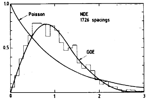
FIG. 1.: Nearest neighbor spacing distribution for the “Nuclear Data Ensemble” comprising 1726 spacings (histogram) versus $s=S/D$ with $D$ the mean level spacing and $S$ the actual spacing. For comparison, the RMT prediction labelled GOE and the result for a Poisson distribution are also shown as solid lines. Taken from Ref. [1].

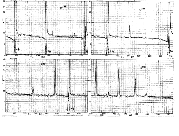
FIG. 2.: Total cross section versus neutron energy for scattering of neutrons on ²³⁸U. The resonances all have the same spin $1/2$ and positive parity. Taken from Ref. [2].

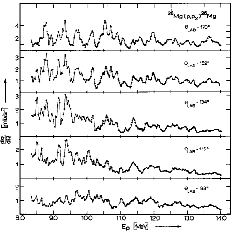
FIG. 3.: Differential cross section at several lab angles versus proton c.m. energy (in MeV) for the reaction ²⁶Mg$(p,p)^{26}$Mg leaving ²⁶Mg in its second excited state. Taken from Ref. [3].

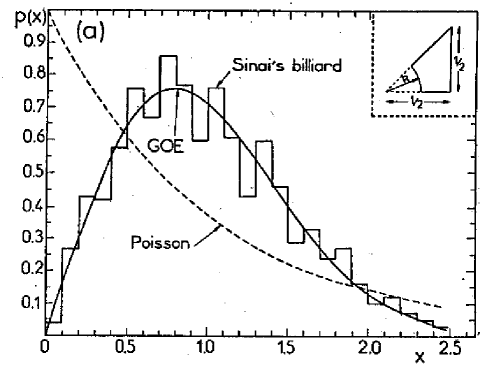
FIG. 4.: The nearest neighbor spacing distribution versus $s$ (defined as in Fig. 1) for the Sinai billiard. The histogram comprises about 1000 consecutive eigenvalues. Taken from Ref. [5].

FIG. 5.: Nearest neighbor spacing distribution versus $s$ (as in Fig. 1) for the hydrogen atom in a strong magnetic field. The levels are taken from a vicinity of the scaled binding energy $\tilde{E}$. Solid and dashed lines are fits, except for the bottom figure which represents the GOE. The transition Poisson $\rightarrow$ GOE is clearly visible. Taken from Ref. [6].

FIG. 6.: Nearest neighbour spacing distribution for elastomechanical modes in an irregularly shaped quartz crystal. Taken from Ref. [7].

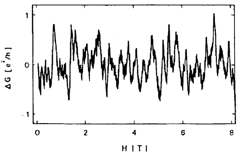
FIG. 7.: The difference $\Delta G$ of the conductance and its mean value, in units of $e^{2}/h$, of a 310 nm wire at a temperature of 0.01 K versus magnetic field strength $H$ in Tesla. Taken from Ref. [8].

These applications of RMT were all in the spirit of Wigner’s original proposal. More recently, RMT has found a somewhat unexpected extension of its domain of application. RMT has become an important tool in the study of systems which are seemingly quite different from complex many–body systems. Examples are: Equilibrium and transport properties of disordered quantum systems and of classically chaotic quantum systems with few degrees of freedom, two–dimensional gravity, conformal field theory, and the chiral phase transition in quantum chromodynamics. Figures 4 to 7 show several cases of interest. The Sinai billiard is the prime example of a fully chaotic classical system. Within statistics, the NNS distribution for the quantum version shown [5] as the histogram in Fig. 4 agrees perfectly with the RMT prediction (solid line). The successful application of RMT is not confined to toy models like the Sinai billiard. Rydberg levels of the hydrogen atom in a strong magnetic field have a spacing distribution [6] which once again agrees with RMT (Fig. 5). The same is true [7] of the elastomechanical eigenfrequencies of irregularly shaped quartz blocks (Fig. 6). And the transmission of (classical or quantum) waves through a disordered medium shows patterns similar to Ericson fluctuations. Figure 7 [8] shows the fluctuations of the conductance of a wire of micrometer size caused by applying an external magnetic field. Such observations and independent theoretical progress paved the way for the rapid development of RMT.

Some of these developments were triggered or at least significantly advanced by the introduction of a new tool into RMT: Efetov’s supersymmetry technique and the ensuing mapping of the random–matrix problem onto a non–linear supersymmetric $\sigma$ model. This advance has, in turn, spurred developments in mathematical physics relating, among other items, to interacting Fermion systems in one dimension (the Calogero–Sutherland model), to supersymmetric Lie algebras, to Fourier transformation on graded manifolds, and to extensions of the Itzykson–Zuber integral.

As the title suggests, we use the term “Random Matrix Theory” in its broadest sense. It stands not only for the classical ensembles (the three Gaussian ensembles introduced by Wigner and the three circular ensembles introduced by Dyson) but for any stochastic modelling of a Hamiltonian using a matrix representation. This comprises the embedded ensembles of French et al. as well as the random band matrices used for extended systems and several other cases. We attempt to exhibit the common concepts underlying these Random Matrix Theories and their application to physical problems.

To set the tone, and to introduce basic concepts, we begin with a historical survey (Sec. II). Until the year 1983, RMT and localization theory (i.e., the theory of disordered solids) developed quite independently. For this reason, we devote separate subsections to the two fields. In the years 1983 and 1984, two developments took place which widened the scope of RMT enormously. First, Efetov’s supersymmetric functional integrals, originally developed for disordered solids, proved also applicable to and useful for problems in RMT. This was a technical breakthrough. At the same time, it led to a coalescence of RMT and of localization theory. Second, the “Bohigas conjecture” established a generic link between RMT and the spectral fluctuation properties of classically chaotic quantum systems with few degrees of freedom. It was these two developments which in our view largely triggered the explosive growth of RMT during the last decade.

Subsequent sections of the review are devoted to a description of this growth. In Sec. III we focus attention on formal developments in RMT. We recall classic results, define essential spectral observables, give a short introduction into scattering theory and supersymmetry, and discuss wavefunction statistics, transitions and parametric correlations. It is our aim to emphasize that RMT, in spite of all its applications, has always been an independent field of research in its own right. In Sec. IV we summarize the role played by RMT in describing statistical aspects of systems with many degrees of freedom. Examples of such systems were mentioned above (atoms, molecules, and nuclei) but also include interacting electrons in ballistic mesoscopic devices. Section V deals with the application of RMT to “quantum chaology”, i.e. to the quantum manifestations of classical chaos. Here, we restrict ourselves to systems with few degrees of freedom. Important examples are mesoscopic systems wherein the electrons move independently and ballistically (i.e., without impurity scattering). Section VI deals with the application of RMT to disordered systems, and to localization theory. This application has had major repercussions in the theory of mesoscopic systems with diffusive electron transport. Moreover, it has focussed theoretical attention on novel issues like the spectral fluctuation properties at the mobility edge. Treating the Coulomb interaction between electrons in such systems forms a challenge which has been addressed only recently. The need to handle the crossover from ballistic to diffusive electron transport in mesoscopic systems has led to a common view of both regimes, and to the discovery of new and universal laws for parametric correlation functions in such systems. However, we neither cover the integer nor the fractional quantum Hall effect. Section VII deals with the numerous applications of RMT in one–dimensional systems of interacting Fermions, in QCD, and in field theory and quantum gravity. Section VIII is devoted to a discussion of the universality of RMT. This concerns the question whether or not certain statistical properties are independent of the specified probability distribution function in matrix space.

In our view, the enormous development of RMT during the last decade signals the birth of a “new kind of statistical mechanics” (Dyson). The present review can be seen as a survey of this emergent field. The evidence is growing that not only disordered but also strongly interacting quantum systems behave stochastically. The combination of stochasticity and general symmetry principles leads to the emergence of general laws. Although not derived from first dynamical principles, these laws lay claim to universal validity for (almost) all quantum systems. RMT is the main tool to discover these universal laws. In Sec. IX, we end with general considerations and speculations on the origins and possible implications of this “new statistical mechanics”.

The breadth of the field is such that a detailed account would be completely beyond the scope of a review paper. As indicated in the title, we focus attention on the concepts, both physical and mathematical, which are either basic to the field, or are common to many (if not all) of its branches. While we cannot aim at completeness, we attempt to provide for the last decade a bibliography which comprises at least the most important contributions. For earlier works, and for more comprehensive surveys of individual subfields, we refer the reader to review articles or reprint collections at appropriate places in the text.

We are painfully aware of the difficulty to give a balanced view of the field. Although we tried hard, we probably could not avoid misinterpretations, imbalances, and outright oversights and mistakes. We do apologize to all those who feel that their work did not receive enough attention, was misinterpreted, or was unjustifyably omitted alltogether.

In each of the nine sections, we have adopted a notation which has maximum overlap with the usage of the literature covered in that section, often at the expense of consistency between different sections. We felt that this approach would best serve our readers. We could not always avoid using the same symbol for different quantities. This is the case, for instance, for the symbol $P$. Most often, $P$ denotes a probability density. Context and argument of the symbol should identify the quantity unambiguously.

We could not have written this review without the continuous advice and help of many people. Special thanks are due to David Campbell, editor of Physics Letters, for having triggered the writing of this paper. We are particularly grateful to J. Ambjørn, C. Beenakker, L. Benet, R. Berkovits, G. Casati, Y. Gefen, R. Hofferbert, H. Köppel, I. Lerner, K. Lindemann, E. Louis, C. Marcus, A. D. Mirlin, R. Nazmitdinov, J. Nygård, A. Richter, T. Seligman, M. Simbel, H. J. Stöckmann, G. Tanner, J.J.M. Verbaarschot, and T. Wettig for reading parts or all of this review, and/or for many helpful comments and suggestions. Part of this work was done while the authors were visiting CIC, UNAM, Cuernavaca, Mexico.

II Historical survey: the period between 1951 and 1983

As mentioned above, in this period RMT and localization theory developed virtually independently, and we therefore treat their histories separately.

After a period of rapid growth during the 1950’s, RMT was almost dormant until it virtually exploded about ten years ago. Our history of RMT therefore consists of three parts. These parts describe (i) the early period (1951 till 1963) in which the basic ideas and concepts were formulated, and the classical results were obtained (Sec. II A); (ii) the period 1963 till 1983 in which the theory was consolidated, relevant data were gathered, and some fundamental open problems came to the surface (Sec. II B); (iii) the almost simultaneous introduction of the supersymmetry method (Sec. II D) and of the Bohigas conjecture (Sec. II E) around 1983.

For a long time, applications of RMT have essentially been confined to nuclear physics. The reason is historical: This was the first area in physics where the available energy resolution was fine enough, i.e. of the order of $D$, and the data set large enough, to display spectral fluctuation properties relevant for tests of RMT. This is why — aside from a description of the technical development of RMT — Secs. II A and II B deal almost entirely with problems in nuclear theory. We will not mention again that here and in other systems, spectroscopic tests of the theory always involve levels of the same spin and parity or, more generally, of the same symmetry class.

After its inception by Anderson in 1958, localization theory received a major boost by the work of Mott and, later, by the application of scaling concepts. This is the history described in Sec. II C. For pedagogical reasons, this section precedes the ones on supersymmetry and chaos.

In this historical review, we refer to review papers wherever possible. We do so at the expense of giving explicit references to individual papers.

A RMT: the early period

Most references can be found in Porter’s book [9] and are not given explicitly. Our account is not entirely historical: History serves as an introduction to the relevant concepts.

In 1951, Wigner proposed the use of RMT to describe certain properties of excited states of atomic nuclei. This was the first time RMT was used to model physical reality. To understand Wigner’s motivation for taking such a daring step, it is well to recall the conceptual development of nuclear theory preceding it.

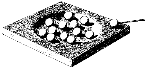
FIG. 8.: Photograph of Niels Bohr’s wooden toy model for compound–nucleus scattering. Taken from Ref.[10].

In the scattering of slow neutrons by medium–weight and heavy nuclei, narrow resonances had been observed. Each of these resonances corresponds to a long–lived “compound state” of the system formed by target nucleus and neutron. In his famous 1936 paper, N. Bohr [10] had described the compound nucleus as a system of strongly interacting neutrons and protons. In a neutron–induced nuclear reaction, the strong interaction was thought to lead to an almost equal sharing of the available energy between all constituents, i.e. to the attainment of quasi–equilibrium. As a consequence of equilibration, formation and decay of the compound nucleus should be almost independent processes. In his appeal to such statistical concepts, Bohr prepared the ground for Wigner’s work. In fact, RMT may be seen as a formal implementation of Bohr’s compound nucleus hypothesis. At the same time, it is remarkable that the concepts and ideas formulated by Bohr have a strong kinship to ideas of classical chaotic motion which in turn are now known to be strongly linked to RMT. This is most clearly seen in Fig. 8 [11] which is a photograph of a wooden model used by Bohr to illustrate his idea. The trough stands for the nuclear potential of the target nucleus. This potential binds the individual nucleons, the constituents of the target, represented as small spheres. An incoming nucleon with some kinetic energy (symbolized by the billard queue) hits the target. The collision is viewed as a sequence of nucleon–nucleon collisions which have nearly the character of hard–sphere scattering.

In the absence of a dynamical nuclear theory (the nuclear shell model had only just been discovered, and had not yet found universal acceptance), Wigner focussed emphasis on the statistical aspects of nuclear spectra as revealed in neutron scattering data. At first sight, such a statistical approach to nuclear spectroscopy may seem bewildering. Indeed, the spectrum of any nucleus (and, for that matter, of any conservative dynamical system) is determined unambiguously by the underlying Hamiltonian, leaving seemingly no room for statistical concepts. Nonetheless, such concepts may be a useful and perhaps even the only tool available to deal with spectral properties of systems for which the spectrum is sufficiently complex. An analogous situation occurs in number theory. The sequence of prime numbers is perfectly well defined in terms of a deterministic set of rules. Nevertheless, the pattern of occurrence of primes among the integers is so complex that statistical concepts provide a very successful means of gaining information on the distribution of primes. This applies, for instance, to the average density of primes (the average number of primes per unit interval), to the root–mean–square deviation from this average, to the distribution of spacings between consecutive primes, and to other relevant information which can be couched in statistical terms.

The approach introduced by Wigner differs in a fundamental way from the standard application of statistical concepts in physics, and from the example from number theory just described. In standard statistical mechanics, one considers an ensemble of identical physical systems, all governed by the same Hamiltonian but differing in initial conditions, and calculates thermodynamic functions by averaging over this ensemble. In number theory, one considers a single specimen — the sequence of primes — and introduces statistical concepts by performing a running average over this sequence. Wigner proceeded differently: He considered ensembles of dynamical systems governed by different Hamiltonians with some common symmetry property. This novel statistical approach focusses attention on the generic properties which are common to (almost) all members of the ensemble and which are determined by the underlying fundamental symmetries. The application of the results obtained within this approach to individual physical systems is justified provided there exists a suitable ergodic theorem. We return to this point later.

Actually, the approach taken by Wigner was not quite as general as suggested in the previous paragraph. The ensembles of Hamiltonian matrices considered by Wigner are defined in terms of invariance requirements: With every Hamiltonian matrix belonging to the ensemble, all matrices generated by suitable unitary transformations of Hilbert space are likewise members of the ensemble. This postulate guarantees that there is no preferred basis in Hilbert space. Many recent applications of RMT use extensions of Wigner’s original approach and violate this invariance principle. Such extensions will be discussed later in this paper.

It is always assumed in the sequel that all conserved quantum numbers like spin or parity are utilized in such a way that the Hamiltonian matrix becomes block–diagonal, each block being characterized by a fixed set of such quantum numbers. We deal with only one such block in many cases. This block has dimension $N$. The basis states in Hilbert space relating to this block are labelled by greek indices like $\mu$ and $\nu$ which run from $1$ to $N$. Since Hilbert space is infinite–dimensional, the limit $N\rightarrow\infty$ is taken at some later stage. Taking this limit signals that we do not address quantum systems having a complete set of commuting observables. Taking this limit also emphasises the generic aspects of the random–matrix approach. Inasmuch as RMT as a “new kind of statistical mechanics” bears some analogy to standard statistical mechanics, the limit $N\rightarrow\infty$ is kin to the thermodynamic limit.

Using early group–theoretical results by Wigner [12], Dyson showed that in the framework of standard Schrödinger theory, there are three generic ensembles of random matrices, defined in terms of the symmetry properties of the Hamiltonian.

(i) Time–reversal invariant systems with rotational symmetry. For such systems, the Hamiltonian matrix can be chosen real and symmetric,

$$H_{mn}=H_{nm}=H^{*}_{mn}.$$ (1)

Time–reversal invariant systems with integer spin and broken rotational symmetry also belong to this ensemble.

(ii) Systems in which time–reversal invariance is violated. This is not an esoteric case but occurs frequently in applications. An example is the Hamiltonian of an electron in a fixed external magnetic field. For such systems, the Hamiltonian matrices are Hermitean,

$$H_{mn}=[H^{\dagger}]_{nm}.$$ (2)

(iii) Time–reversal invariant systems with half–integer spin and broken rotational symmetry. The Hamiltonian matrix can be written in terms of quaternions, or of the Pauli spin matrices $\sigma_{\gamma}$ with $\gamma=1,2,3$. The Hamiltonian has the form

$$H^{(0)}_{nm}1_{2}-i\sum_{\gamma=1}^{3}H^{(\gamma)}_{nm}\sigma_{\gamma},$$ (3)

where all four matrices $H^{(\gamma)}$ with $\gamma=0,\ldots,3$ are real and where $H^{(0)}$ is symmetric while $H^{(\gamma)}$ with $\gamma=1,2,3$ are antisymmetric.

In all three cases the probability of finding a particular matrix is given by a weight function $P_{N\beta}(H)$ times the product of the differentials of all independent matrix elements. Both the symmetry properties (1), (2), and (3), and the weight functions $P_{N\beta}(H)$ for $\beta=1,2,4$ are invariant under orthogonal, unitary, and symplectic transformations of the Hamiltonian, respectively. The index $\beta$ is often used to specify the ensemble altogether. In a sense specified by Dyson, the three ensembles are fundamentally irreducible and form the basis of all that follows. Novel ensembles not contained in this list may arise [13, 14] when additional symmetries or constraints are imposed. Such ensembles have recently been discussed in the context of Andreev scattering [15], and of chiral symmetry [16].

The choice $P_{N\beta}(H)=1$ would be consistent with the symmetry requirements but would lead to divergent integrals. For the Gaussian ensembles considered by Wigner, the weight functions $P_{N\beta}$ are chosen to have Gaussian form,

$$P_{N\beta}(H)\propto\exp\left(-\frac{\beta N}{\lambda^{2}}\,{\rm tr}H^{2}\right).$$ (4)

We have suppressed a normalization factor, see Sec. III A 2. The constant $\lambda$ is independent of $N$. The factor $N$ ascertains that the spectrum of the ensemble remains bounded in the limit $N\rightarrow\infty$. The independent elements of the Hamiltonian are independent random variables; the distributions factorize. For a more formal discussion of the three Gaussion ensembles we refer to Sec. III A.

The choice (4) defines the three canonical ensembles: The Gaussian orthogonal ensemble (GOE) with $\beta=1$. the Gaussian unitary ensemble (GUE) with $\beta=2$, and the Gaussian symplectic ensemble (GSE) with $\beta=4$. These ensembles have similar weight functions $P_{N\beta}$ but different symmetries, and consequently different volume elements in matrix space. As mentioned before, this review covers a variety of Random Matrix Theories. For clarity, we refer to the ensembles introduced above jointly as to Gaussian Random Matrix Theory (GRMT).

The introduction of RMT as a theory of physical systems poses two questions. (a) How are predictions on observables obtained from RMT? (b) How are such predictions compared with physical reality? A third question arises when we note that the requirements (i) to (iii) defining the three classical ensembles are based on general symmetry principles and their quantum–mechanical implementation, while the choice of the Gaussian functions (4) was dictated by convenience. We must therefore ask: (c) Are the conclusions derived from the Gaussian ansatz generally valid, i.e. independent of the Gaussian form (which would then indeed serve only as a convenient vehicle)?

Basic for most applications of GRMT is the distinction between average quantities and their fluctuations. Because of the cutoff due to the Gaussian weight factors, all three Gaussian ensembles defined above have a spectrum which in the limit $N\rightarrow\infty$ is bounded and has length $4\lambda$. In the interval $-2\lambda\leq E\leq 2\lambda$, the average level density has the shape of a semicircle (cf. Eq. (7) below). For most physical systems, a bounded spectrum with semicircle shape is totally unrealistic. Therefore, GRMT is generically useless for modelling average properties like the mean level density. The situation is different for the statistical fluctuations around mean values of observables. Since there are $N$ levels in the spectrum, $D\sim N^{-1}$ tends to zero as $N\rightarrow\infty$. In this limit, fluctuation properties may become independent of the form of the global spectrum and of the choice of the Gaussian weight factors, and may attain universal validity. This is the expectation held upon employing GRMT, see in particular Sec. VIII. The wide range of successful applications of RMT in its Gaussian form has for a long time suggested that this expectation is justified. Balian [17] derived the three Gaussian ensembles from a maximum entropy principle, postulating the existence of a second moment of the Hamiltonian. His derivation shows that in the absence of any further constraints, the Gaussian weight factors are the must natural ones to use. This result and numerical studies gave further credence to the belief that fluctuation properties should not depend on the Gaussian form of the weight factors. There is now also direct evidence for this assertion. It is presented in Sec. VIII.

GRMT can thus be used to predict fluctuations of certain observables. The general scheme is this: The average of the observable over the ensemble serves as input, and the fluctuation properties are derived from GRMT. Examples are local level correlation functions (with the average level density as input to define the physical value of $N/\lambda$), distribution laws and local correlation functions for eigenvectors (which are usually measured by coupling to some external field, the average of the square of the coupling matrix element serving as input), etc. We will encounter numerous examples of this type as we proceed. In some select cases, it is possible to work out the fluctuation properties of the observable completely, and to calculate the entire distribution function over the ensemble. In most cases, however, this goal is too ambitious, and one has to settle for the first few moments of the distribution.

In comparing such predictions with experiment, we must relate the average over the (fictitious) ensemble given by GRMT with information on a given system. Here, an ergodic hypothesis is used. It says that the ensemble average is equal to the running average, taken over a sufficiently large section of the spectrum, of almost any member of the ensemble. In specific cases, this ergodic hypothesis has been proved [18].

It is clear that RMT cannot ever reproduce a given data set in its full detail. It can only yield the distribution function of, and the correlations between, the data points. An example is the nuclear level spectrum at neutron threshold, the first case ever studied in a statistically significant fashion. The actual sequence of levels observed experimentally remains inaccessible to RMT predictions, while the distribution of spacings and the correlations between levels can be predicted. The same holds for the stochastic fluctuations of nuclear cross sections, for universal conductance fluctuations of mesoscopic probes, and for all other applications of RMT.

GRMT is essentially a parameter–free theory. Indeed, the only parameter ($\lambda$) is fixed in terms of the local mean level spacing of the system under study. The successful application of GRMT to data shows that these data fluctuate stochastically in a manner consistent with GRMT. Since GRMT can be derived from a maximum entropy principle [17], this statement is tantamount to saying that the data under study carry no information content. It is an amazing fact that out of this sheer stochasticity, which is only confined by the general symmetry principles embodied in GRMT, the universal laws alluded to above do emerge.

The distribution of the eigenvalues and eigenvectors is obviously a central issue in applications of GRMT. To derive this distribution, it is useful to introduce the eigenvalues $E_{\mu}$ and the eigenvectors of the matrices as new independent variables. The group–theoretical aspects of this procedure were probably first investigated by Hua [19], cf. also Ref. [20]. After this transformation, the probability measures for the three Gaussian ensembles factorize. One term in the product depends only on the eigenvalues, the other, only on the eigenvectors (angles). Moreover, because of the assumed invariance properties, the functions $P_{N\beta}$ depend on the eigenvalues only. Therefore, eigenvectors and eigenvalues are uncorrelated random variables. The form of the invariant measure for the eigenvectors implies that in the limit $N\rightarrow\infty$, these quantities are Gaussian– distributed random variables.

Following earlier work by Scott, Porter and Thomas suggested this Gaussian distribution for the eigenvectors in 1956. Their paper became important because it triggered many comparisons between GRMT predictions and empirical data. In nuclear reaction theory, the quantities which determine the strength of the coupling of a resonance to a particular channel are the “reduced partial width amplitudes”, essentially given by the projection of the resonance eigenfunction onto the channel surface. Identification of the resonance eigenfunctions with the eigenfunctions of the GOE implies that the reduced partial width amplitudes have a Gaussian probability distribution centered at zero, and that the reduced partial widths (the squares of the partial width amplitudes) have a $\chi^{2}$ distribution with one degree of freedom (the “Porter–Thomas distribution”). This distribution obtains directly from the volume element in matrix space and holds irrespective of the choice of the weight function $P_{N1}(H)$. It is given in terms of the average partial width which serves as input parameter.

For the eigenvalues, the invariant measure takes the form $(\beta=1,2,4)$

$$P_{N\beta}(E_{1},\ldots,E_{N})\prod_{m>n}|E_{m}-E_{n}|^{\beta}\prod_{l=1}^{N}dE_{l}.$$ (5)

This expression displays the famous repulsion of eigenvalues which becomes stronger with increasing $\beta$. (Eigenvalue repulsion as a generic feature of quantum systems was first discussed by von Neumann and Wigner [21]. The arguments used in this paper explain the ${\beta}$–dependence of the form (5)). We note that this level repulsion is due entirely to the volume element in matrix space, and independent of the weight function: It influences local rather than global properties. It turned out to be very difficult to deduce information relevant for a comparison with experimental data from Eq. (5). Such a comparison typically involves the correlation function between pairs of levels, or the distribution of spacings between nearest neighbors. The integrations over all but a few eigenvalues needed to derive such information were found to be very hard.

Lacking exact results, and guided by the case $N=2$, Wigner proposed in 1957 a form for the distribution $p(s)$ of spacings of neighboring eigenvalues, i.e. for the nearest neighbor spacing distribution mentioned in the Introduction. Here, $s$ is the level spacing in units of the local mean level spacing $D$. This “Wigner surmise”, originally stated for $\beta=1$, has the form

$$p_{\beta}(s)=a_{\beta}s^{\beta}\exp(-b_{\beta}s^{2}).$$ (6)

The constants $a_{\beta}$ and $b_{\beta}$ are given in Eq. (77) of Sec. III B 2. The Wigner surmise shows a strong, $\beta$–dependent level repulsion at small spacings (this is a reflection of the form (5)), and a Gaussian falloff at large spacings. This falloff has nothing to do with the assumed Gausian distribution of the ensembles and stems directly from the assumed form of the volume element in matrix space. The solid line in Fig. 1 shows the $s$–dependence of $p(s)$ for the orthogonal case.

In the same paper, Wigner also derived the semicircle law mentioned above. As a function of energy $E$, the average level density $\rho=D^{-1}$ is given by

$$\rho(E)=\frac{N}{\pi\lambda}\sqrt{1-(E/(2\lambda))^{2}}.$$ (7)

Later, Pastur [22] derived a quadratic equation for the averaged retarded or advanced Green function. This equation coincides in form with the scalar version of the saddle point equation (122) of the non–linear $\sigma$–model and yields for $\rho(E)$ the semicircle law (7).

The difficulties encountered in calculating spectral properties of GRMT were overcome in 1960 when M. L. Mehta introduced the method of orthogonal polynomials, summarized in his book [23]. Mathematically, his methods are related to Selberg’s integral. Mehta’s work provided the long–missing tool needed to calculate the spectral fluctuation properties of the three canonical ensembles, and therefore had an enormous impact on the field. Mehta could not only prove earlier assertions but also obtained many new results. For instance, Gaudin and Mehta derived the exact form of the nearest neighbour spacing distribution. The Wigner surmise turns out to be an excellent approximation to this distribution. The method of orthogonal polynomials has continued to find applications beyond the canonical ensembles.

GRMT is conceived as a generic theory and should apply beyond the domain of nuclear physics. Early evidence in favor of this assertion, and perhaps the earliest evidence ever in favor of the nearest neighbor spacing distribution, was provided in 1960 by Porter and Rosenzweig. These authors analyzed spectra in complex atoms.

In a series of papers written between 1960 and 1962, Dyson developed RMT much beyond the original ideas of Wigner. Aside from showing that there are three fundamental ensembles (the unitary, orthogonal and symplectic one), he contributed several novel ideas. As an alternative to the Gaussian ensembles defined above, he introduced the three “circular ensembles”, the circular unitary ensemble (CUE), the circular orthogonal ensemble (COE), and the circular symplectic ensemble (CSE). In each of these ensembles, the elements are unitary matrices of dimension $N$ rather than the Hamiltonian matrices used in Wigner’s ensembles. Since the spectra of all three ensembles are automatically confined to a compact manifold (the eigenvalues exp$[i\theta_{\mu}]$ with $\mu=1,\ldots,N$ of unitary matrices are located on the unit circle in the complex plane), there is no need to introduce the (arbitrary) Gaussian weight factors of Eq. (4). This removes an ambiguity of the Gaussian ensembles and simplifies the mathematical problems. Unfortunately, these advantages are partly compensated by the fact that the physical interpretation of the eigenvalues of the circular ensembles is not obvious.

We briefly give the mathematical definitions of the three circular ensembles here because they will not be discussed in detail in Sec. III. Each circular ensemble is defined by the same invariance postulate as the corresponding Gaussian ensemble.

(i) The COE consists of symmetric unitary matrices $S$ of dimension $N$. Each such matrix $S$ can be written as $S=U^{T}U$ where $U$ is unitary and $T$ denotes the transpose. To define the measure, we consider an infinitesimal neighborhood of $S$ given by $S+dS=U^{T}(1_{N}+idM)U$ where $dM$ is infinitesimal, real and symmetric. Let $d\mu_{ij}$ with $1\leq i\leq j\leq N$ denote the differentials of the elements of the matrix $M$. Then the measure $\mu(dS)$ is defined by $\mu(dS)=\prod_{i\leq j}d\mu_{ij}$, and the COE has the probability measure

$$P(dS)={\mu(dS)\over\int\mu(dS)}.$$ (8)

The COE is invariant under every automorphism $S\rightarrow U^{\prime T}SU^{\prime}$ where $U^{\prime}$ is unitary.

(ii) The CUE consists of unitary matrices $S$ of dimension $N$. Each such matrix can be written as the product $S=UV$ of two unitary matrices $U$ and $V$ so that $S+dS=U(1_{N}+idH)V$ where $dH$ is infinitesimal Hermitean. The measure $\mu(dS)$ is defined by $\mu(dS)=\prod_{i\leq j}d{\rm Re}\mu_{ij}\prod_{i<j}d{\rm Im}\mu_{ij}$ where $d\mu_{ij}$ denotes the differentials of the elements of the matrix $H$. With this changed definition of $\mu(dS)$, the probability measure again has the form of Eq. (8). The CUE is invariant under every automorphism $S\rightarrow U^{\prime}SV^{\prime}$ where $U^{\prime},V^{\prime}$ are unitary.

(iii) The CSE consists of unitary matrices $S$ of dimension $N$ which have the form $S=U^{R}U$ where $U$ is unitary, and where $R$ denotes the dual, defined by the combined operation of time–reversal ($K$) and transposition, $U^{R}=KU^{T}K^{-1}$. We have $S+dS=U^{R}(1_{N}+idM)U$ where $dM$ is infinitesimal, quaternion–real and self–dual. The measure $\mu(dS)$ is defined in terms of the differentials $d\mu_{ij}^{\gamma},\ \gamma=0,\ldots,3$ of the four matrices $M^{\gamma}$ of the quaternion decomposition of $M$ as $\mu(dS)=\prod_{i}d\mu_{ii}^{0}\prod_{\gamma=0}^{3}\prod_{i\leq j}d\mu_{ij}^{\gamma}$. With this changed definition of $\mu(dS)$, the probability measure again has the form of Eq. (8). The CSE is invariant under every automorphism $S\rightarrow W^{R}SW$ where $W$ is unitary.

The phase angles $\theta_{\mu}$ of Dyson’s ensembles are expected to have the same local fluctuation properties as the eigenvalues $E_{\mu}$ of the corresponding Gaussian ensembles. This expectation is borne out by calculating the invariant measure. It carries the factor $\prod_{\mu>\nu}|\exp(i\theta_{\mu})-\exp(i\theta_{\nu})|^{\beta}$, in full analogy to Eq. (5). Using the Gaudin–Mehta method, Dyson was able to derive the $k$–level correlation function (i.e. the probability density for $k$ phase angles $\theta_{\mu}$ with $\mu=1,\ldots,k\ll N$, irrespective of the position of all others). These functions coincide with the corresponding expressions for the Gaussian ensembles found by Mehta, strengthening the belief that the Gaussian weight factor is immaterial for local fluctuation properties. The explicit formulas for the two–level correlation functions can be found in Sec. III A 5.

Aside from furnishing useful alternatives to the Gaussian ensembles, the circular ensembles have found direct application in stochastic scattering theory since the elements of the ensembles — the unitary matrices $S$ — can be viewed as scattering matrices.

Dyson also noticed an interesting connection between GRMT and a classical Coulomb gas. For the Gaussian ensembles, the factors appearing in Eq. (5) can be written in the form

$$\exp\left(-\beta N\sum_{n=1}^{N}\left[\frac{E_{n}}{\lambda}\right]^{2}+\frac{\beta}{2}\sum_{m>n}\ln\left[\frac{E_{m}-E_{n}}{\lambda}\right]^{2}\right).$$ (9)

From a thermodynamic point of view, this expression is the free energy of a static Coulomb gas of $N$ particles in one dimension with positions $E_{1},\ldots,E_{N}$ and temperature $\beta^{-1}$. The gas is confined by a harmonic oscillator potential, which is absent for the circular ensembles originally considered by Dyson. The parameter $\beta$ plays the role of an inverse temperature. This analogy helps to understand the fluctuation properties of the spectrum. Both the level repulsion at short distance and the long–range stiffness of the spectrum (see Eq. (10) and the remarks following it) characteristic of GRMT become intuitively obvious.

Another important idea in Dyson’s work relates to cases of slightly broken symmetries or invariance properties. The ensembles considered so far all correspond to exactly obeyed symmetries and invariances. In many applications of RMT, it is necessary to consider cases of slight symmetry breaking. This is true, for instance, for isospin–mixing in nuclei, for parity violation in nuclei, or for time–reversal invariance breaking in solids. These effects are caused by the Coulomb interaction, the weak interaction, and an external magnetic field acting on the electrons, respectively. Such cases can be modeled by adding to the ensemble describing the conserved symmetry (or invariance) another one, which violates the symmetry (or invariance) and has relative strength $t$ with respect to the first. More precisely, the variances of the matrix elements in the second ensemble differ by a factor $t^{2}$ from those in the first. By generalizing the static Coulomb gas model of the last paragraph to a dynamical one, where the $N$ particles, in addition to their mutual repulsion, are also subject to dissipative forces, Dyson arrived at a Brownian motion model for the eigenvalues of a random matrix. Starting at time $t=0$ with the case of pure symmetry, and letting the Brownian motion proceed, the eigenvalues move under the influence of the symmetry–breaking ensemble. The Brownian–motion model has found important applications in recent years.

We refer to the Gaussian and the circular ensembles jointly as to classical Random Matrix Theory (cRMT).

In comparing cRMT results with experiment, it is useful to have available statistical measures tailored to the fact that the data set always comprises a finite sequence only. In 1963, Dyson and Mehta introduced several statistical measures (the “Dyson–Mehta statistics”) to test a given sequence of levels for agreement with cRMT. These measures have found wide application. One important example is the $\Delta_{3}$ statistic, which will be discussed in detail in Sec. III B 3. Let $\eta(E)$ be the number of energy levels in the interval $[-\infty,E]$, and let us assume that the spectrum has been “unfolded” so that the local average level density is constant (independent of $E$). On this unfolded, dimensionless energy scale $\xi$, the number of levels in the interval $[-\infty,\xi]$ is given by $\widehat{\eta}(\xi)$. The $\Delta_{3}$ statistic

$$\Delta_{3}(L)=\left\langle\min_{A,B}\frac{1}{L}\int_{\xi_{s}}^{\xi_{s}+L}\left(\widehat{\eta}(\xi)-A\xi-B\right)^{2}d\xi\right\rangle_{\xi_{s}}.$$ (10)

measures how well the staircase function $\widehat{\eta}(\xi)$ can be locally approximated by a straight line. The angular brackets in Eq. (10) indicate an average over $\xi_{s}$. If subsequent spacings of nearest neighbors were uncorrelated, $\Delta_{3}(L)$ would be linear in $L$, $\Delta_{3}(L)=L/15$. An essential property of RMT is the logarithmic dependence of $\Delta_{3}(L)$ on $L$. It is often referred to as the ‘stiffness’ of the spectrum (cf. the remarks below Eq. (5)). Explicit expressions for $\Delta_{3}(L)$ in all three symmetry classes are given in Sec. III B 3.

As remarked above, the compound–nucleus resonances observed in slow neutron scattering are prime candidates for applications of GRMT. By implication, the neutron scattering cross section in this energy range is expected to be a random process. In the Introduction, it was pointed out that already a few MeV above neutron threshold, the resonances overlap strongly. Nonetheless, the cross section should still be stochastic. Using a simple statistical model for the nuclear scattering matrix, Ericson proposed in 1963 that in this domain, cross–section fluctuations with well–defined properties (“Ericson fluctuations”) should exist. This proposal was made before the necessary experimental resolution and the data shown in Fig. 3 became available. The proposal gave a big boost to nuclear reaction studies, see the review in Ref. [24]. For quite some time, the connection between Ericson’s model and cRMT remained an open question, however.

B From 1963 to 1982: consolidation and application

In this period, nuclear reaction data became available which permitted the first statistically significant test of GRMT predictions on level fluctuations. Ericson’s prediction of random cross–section fluctuations was confirmed, and many reaction data in the domain of strongly overlapping resonances were analyzed using his model. Theorists tackled the problem of connecting Ericson fluctuations with GRMT. Two–body random ensembles and embedded ensembles were defined as a meaningful extension of GRMT. Symmetry breaking became a theoretical issue in GRMT. The results were used to establish upper bounds on the breaking of time–reversal symmetry in nuclei.

Much of this work is reviewed in Refs. [18, 25].

A significant test of GRMT predictions requires a sufficiently large data set. Collecting such a set for the sole purpose of testing stochasticity may seem a thankless task. The opposite is the case. It is important to establish whether stochasticity as formulated in GRMT does apply in a given system within some domain of excitation energy, and to what extent this is the case. Moreover, once the applicability of GRMT is established, there is no room left for spectroscopic studies involving a level–by–level analysis. Indeed, Balian’s derivation of GRMT from a maximum–entropy principle [17] shows that spectroscopic data taken in the domain of validity of GRMT carry no information content.

In the 1970’s, a determined experimental effort produced data on low–energy neutron scattering by a number of heavy nuclei, and on proton scattering near the Coulomb barrier by several nuclei with mass numbers around $50$. The number of levels with the same spin and parity seen for any one of these target nuclei ranged typically from $100$ to $200$. In 1982, the totality of these data was combined into the “Nuclear Data Ensemble” comprising $1726$ level spacings. This ensemble was tested by Haq, Pandey and Bohigas [26, 1] for agreement with the GOE (the relevant ensemble for these cases). They used the nearest neighbor spacing distribution and the $\Delta_{3}$ statistic. This analysis produced the first statistically significant evidence for the agreement of GOE predictions and spectral properties of nuclei, see Fig. 1.

The advent of electrostatic accelerators of sufficiently high energy and of sufficiently good energy resolution (which must be better than the average width $\Gamma$ of the compound–nucleus resonances) made it possible at that time to detect Ericson fluctuations [24] in nuclear cross sections, see Fig. 3. As a function of incident energy, the intensity of particles produced in a nuclear reaction at fixed scattering angle shows random fluctuations. An evaluation of the intensity autocorrelation versus incident energy yields the average lifetime $\hbar/\Gamma$ of the compound nucleus, and the autocorrelation versus scattering angle yields information on the angular momenta relevant for the reaction. ¿From the variance one finds the ratio of “direct reactions”, i.e. of particles emitted without delay, to the typically long–delayed compound–nucleus reaction contribution. The “elastic enhancement factor” favors elastic over inelastic compound–nucleus reactions and is the forerunner of the “weak localization correction” in mesoscopic physics. The authors of reference [24] were well aware of the fact that the phenomena discovered in nuclear reactions are generic. And indeed, most of the concepts developed within the theory of Ericson fluctuations have later resurfaced in different guise when the theory of wave propagation through disordered media was developed, and was applied to chaotic and disordered mesoscopic conductors, and to light propagation through media with a randomly varying index of refraction.

At the same time, intense theoretical efforts were undertaken to give a solid foundation to Ericson’s model, and to connect it with cRMT [25]. This was necessary in order to obtain a unified model for fluctuation properties of nuclear cross sections in the entire range of excitation energies extending from $\Gamma\ll D$ (i.e. neutron threshold where GRMT was known to work) till the Ericson domain $\Gamma\gg D$. The approaches started from two different hypotheses.

(i) The random Hamiltonian approach.

Formal theories of nuclear resonance reactions express the scattering matrix $S$ in terms of the nuclear Hamiltonian $H$, so that $S=S(H)$. Since RMT is supposed to model the stochastic properties of $H$, an ensemble of scattering matrices was obtained by replacing the nulear Hamiltonian by the GOE, i.e. by writing $S=S$(GOE). For example, the shell–model approach to nuclear reactions [27] yields for the elements $S_{ab}(E)$ of the scattering matrix

$$S_{ab}(E)=\delta_{ab}-2i\pi\sum_{\mu\nu}W_{a\mu}(D^{-1}(E))_{\mu\nu}W_{\nu b}.$$ (11)

Here, $E$ is the energy, and $a,b$ refer to the physical channels. The indices $\mu$ and $\nu$ of the inverse propagator $D_{\mu\nu}$ refer to a complete set of orthonormal compound nucleus states, and $D$ (not to be confused with the mean level spacing) has the form

$$D_{\mu\nu}(E)=E\delta_{\mu\nu}-H_{\mu\nu}+i\pi\sum_{c}W_{\mu c}W_{c\nu}.$$ (12)

We have omitted an irrelevant shift function. The symbol $H_{\mu\nu}$ stands for the projection of the nuclear Hamiltonian onto the set of compound nucleus states, and the matrix elements $W_{\mu a}(E)$ describe the coupling between these states and the channels $a$. Equations (11,12) are generically valid. By assuming that $H$ is a member of a random–matrix ensemble, $S$ becomes an ensemble of scattering matrices, and the challenge consists in calculating ensemble–averaged cross sections and correlation functions. Work along these lines was carried out by Moldauer, by Agassi et al., by Feshbach et al., and by many others. Inter alia, this approach led to an asymptotic expansion kin to impurity perturbation theory in condensed matter physics. It is valid for $\Gamma\gg D$ and uses the assumption that the GRMT eigenvalue distribution can be replaced by a model with fixed nearest neighbor spacings (“picket fence model”). In this framework, Ericson’s results could be derived. However, all attempts failed to obtain a unified theoretical GRMT treatment valid in the entire regime from $\Gamma\ll D$ till $\Gamma\gg D$. The methods developed by Mehta which had proven so successful for level correlations did not seem to work for the more complex problem of cross–section fluctuations.

Much theoretical attention was also paid to reactions at energies beyond the Ericson regime where an extension of RMT is needed to describe physical reality. Indeed, the application of RMT to transport processes (like cross sections) implies some sort of equilibrium assumption: By virtue of the orthogonal invariance of the GOE, all states of the compound system are equally accessible to an incident particle, and a preferred basis in Hilbert space does not exist. This assumption is justified whenever the “internal equilibration time” $\tau_{eq}$ needed to mix the states actually populated in the first encounter of projectile and target with the rest of the system is small compared with the time $\hbar/\Gamma$ for particle emission. But $\tau_{eq}$ changes little with energy while $\hbar/\Gamma$ decreases nearly exponentially over some energy interval. At energies above the Ericson regime there exists a domain where decay happens while the system equilibrates. This is the domain of “precompound” or “preequilibrium” reactions. It requires an extension of RMT using a preferred basis in Hilbert space, reflecting the ever increasing complexity of nuclear configurations reached from the incident channel in a series of two–body collisions. Formally, this extension of RMT is a forerunner of and bears a close relationship to the modelling of quasi one–dimensional conductors in terms of random band matrices. In both cases, we deal with non–ergodic systems where a novel energy (or time) scale — the equilibration time or, in disordered solids, the diffusion time — comes into play.

(ii) The random $S$ matrix approach.

A maximum–entropy approach for the scattering matrix kin to Balian’s derivation of GRMT was developed by Mello, Seligman and others. A closed expression for the probability distribution of the elements of the scattering matrix was derived for any set of input parameters (the average elements of $S$). Unfortunately, the result was too unwieldy to be evaluated except in the limiting cases of few or very many open channels. Moreover, parametric correlation functions, e.g. the correlation between two elements of the scattering matrix at different energies, seem not accessible to this approach. Under the name “random transfer matrix approach”, a similar approach has later found wide application in the theory of disordered quasi one–dimensional conductors, cf. Sec. VI C 2. Here again, the calculation of parametric correlation functions has been fraught with difficulties.

The random $S$ matrix approach has the virtue of dealing directly with the elements of the $S$ matrix as stochastic variables. Thereby it avoids introducing a random Hamiltonian in the propagator as done in Eqs. (11,12) and the ensuing difficulties in calculating ensemble averages. This very appealing feature is partly offset by the difficulties in calculating parametric correlations.

A basic criticism leveled against GRMT relates to the fact that in most physical systems, the fundamental interaction is a two–body interaction. In a shell–model basis, this interaction has vanishing matrix elements between all states differing in the occupation numbers of more than two single–particle states. Therefore, the interaction matrix is sparse. In an arbitrary (non–shell model) basis, this implies that the number of independent matrix elements is much smaller than in GRMT, where the coupling matrix elements of any pair of states are uncorrelated random variables. This poses the question whether GRMT predictions apply to systems with two–body forces. It is also necessary to determine whether the two–body matrix elements are actually random. Another problem consists in understanding how a random two–body force acts in a many–Fermion Hilbert space. This problem leads to the question of how information propagates in spaces of increasing complexity. These problems were tackled mainly by French and collaborators [18] and led to “statistical nuclear spectroscopy” as an approach to understand the workings of the two–body residual interaction of the nuclear shell model in large, but finite, shell–model spaces. Specifically, it was shown that in the shell model, the matrix elements of the two–body force are random and have a Gaussian distribution. The mathematical problem of handling such random two–body forces was formulated by introducing the “embedded ensembles”: A random $m$–body interaction operates in a shell–model space with $K$ Fermions where $m<K$. The propagation of the two–body force in complex spaces was investigated with the help of moments methods. It was shown numerically that for $m=2$, the spectral fluctuation properties of such an ensemble with orthogonal symmetry are the same as for the GOE. The last result shows that GOE can meaningfully be used in predicting spectral fluctation properties of nuclei and other systems governed by two–body interactions (atoms and molecules). Nonetheless, embedded ensembles rather than GRTM would offer the proper way of formulating statistical nuclear spectroscopy. Unfortunately, an analytical treatment of the embedded ensembles is still missing.

In the early 80’s, Mehta and Pandey [28, 29] made a significant advance in the theoretical treatment of GRMT. Their work established for the first time the connection between GRMT, field theory, and the Itzykson–Zuber integral. They succeeded in extending the orthogonal polynomial method to the problem of symmetry breaking. In this way, they showed that the nearest neighbor spacing distribution (NNS) could be used as a test of time–reversal invariance in nuclei. The basic idea is that for small spacings, the presence of an interaction breaking time–reversal symmetry would change the linear slope of NNS characteristic of the GOE into a quadratic one typical for the GUE, cf. Eq. (6). To work out this idea, it is necessary to define a random ensemble which allows for the GOE $\rightarrow$ GUE crossover transition. The ensemble defined by Mehta and Pandey for this purpose has the form

$$H_{nm}=H_{nm}^{\rm GOE}+i\sqrt{t/N}H_{nm}^{A}.$$ (13)

Here, $H^{GOE}$ is the GOE, and $H^{A}$ is the ensemble of real antisymmetric Gaussian distributed matrices having the same variance as the GOE. For $t=0$, the ensemble (13) coincides with the GOE, while for $t=N$, it coincides with the GUE. Writing the strength parameter in the form $(t/N)^{1/2}$ is motivated by the following consideration. The perturbation $(t/N)^{1/2}H^{A}$ is expected to influence the local fluctuation properties of the spectrum (those on the scale $D$) for values of $t$ such that the mean–square matrix element of the perturbation is of order $D^{2}$. From Eq. (7), this implies $(t/N)(\lambda^{2}/N)\sim D^{2}\sim(\pi\lambda/N)^{2}$, or $t\sim 1$. This argument shows that the local fluctuation properties are extremely sensitive to a symmetry–breaking perturbation. The results obtained by Mehta and Pandey were used by French et al. to obtain an upper bound on time–reversal symmetry breaking in nuclei.

A similar problem arises from the Coulomb interaction. This interaction is weak compared to the nuclear force and leads to a small breaking of the isospin quantum number. The random–matrix model needed for this case is different from Eq. (13), however. Indeed, without Coulomb interaction the Hamiltonian is block diagonal with respect to the isospin quantum number. In the simplest but realistic case of the mixing of states with two different isospins, it consists of two independent GOE blocks. The isospin–breaking interaction couples the two blocks. The strength parameter of this coupling again scales with $N^{-1/2}$. For spectral fluctuations, this crossover transition problem has not yet been solved analytically (except for the GUE case) whereas an analytical treatment has been possible for nuclear reactions involving isospin symmetry breaking. This case is, in fact, the simplest example for the precompound reaction referred to above. The results provided an ideal tool for the study of symmetry breaking in statistical nuclear reactions. The data gave strong support to the underlying statistical model [30].

We conclude this historical review with a synopsis. RMT may be viewed as a new kind of statistical mechanics, and there are several formal aspects which support such a view. First, RMT is based on universal symmetry arguments. In this respect it differs from ordinary statistical mechanics which is based on dynamical principles; this is the fundamental novel feature of RMT. It is linked to the fact that in RMT, the ensembles consist of physical systems with different Hamiltonians. Second, the Gaussian ensembles of RMT can be derived from a maximum entropy approach. The derivation is very similar to the way in which the three standard ensembles (microcanonical, canonical and grand canonical ensemble) can be obtained in statistical mechanics. Third, the limit $N\rightarrow\infty$ is kin to the thermodynamic limit. Fourth, in relating results obtained in the framework of RMT to data, an ergodic theorem is used. It says that the ensemble average of an observable is — for almost all members of the ensemble — equal to the running average of the same observable taken over the spectrum of a single member of the ensemble. In statistical mechanics, the ergodic theorem states the equality of the phase–space average of an observable and the average of the same observable taken along a single trajectory over sufficiently long time. Finally, the elements of the GRMT matrices generically connect all states with each other. This is a consequence of the underlying (orthogonal, unitary or symplectic) symmetry of GRMT and is reminiscent of the equal a priori occupation probability of accessible states in statistical mechanics. The assumption is valid if the time scale for internal equilibration is smaller than all other time scales.

In the period from 1963 till 1982, the evidence grew strongly that both in nuclear spectrocopy and in nuclear reaction theory, concepts related to RMT are very successful. Two elements were missing, however: (i) A compelling physical argument was lacking why GRMT was such a successful model. Of course, GRMT is a generic theory. But why does it apply to nuclei? More precisely, and more generally: What are the dynamical properties needed to ensure the applicability of GRMT to a given physical system? (ii) Both in nuclear spectroscopy and in nuclear reaction theory, the mathematical tools available were insufficient to answer all the relevant questions analytically, and novel techniques were needed.

C Localization theory

It may be well to recall our motivation for including localization theory in this historical survey. Localization theory deals with the properties of electrons in disordered materials. Disorder is simulated by a random potential. The resulting random single–particle Hamiltonian shares many features with an ensemble of random matrices having the same symmetry properties. In fact, after 1983 the two fields – RMT and localization theory – began to coalesce. A review of localization theory was given by Lee and Ramakrishnan [31] in 1985. Here, we focus on those elements of the development which are pertinent to our context, without any claim of completeness.

The traditional quantum–mechanical description of the resistance of an electron in a metal starts from Bloch waves, the eigenfunctions of a particle moving freely through an ideal crystal. The resistance is due to corrections to this idealized picture. One such correction is caused by impurity scattering. The actual distribution of impurity scatterers in any given sample is never known. Theoretical models for impurity scattering therefore use statistical concepts which are quite similar to the ones used in RMT. The actual impurity potential is replaced by an ensemble of impurity potentials with some assumed probability distribution, and observables are calculated as averages over this ensemble. It is frequently assumed, for instance, that the impurity potential $V(\vec{r})$ is a Gaussian random process with mean value zero and second moment

$$\overline{V(\vec{r}_{1})V(\vec{r}_{2})}=\frac{1}{2\pi\nu\tau}\delta(\vec{r}_{1}-\vec{r}_{2}).$$ (14)

Here, the ensemble average is indicated by a bar, $\nu=(V\Delta)^{-1}$ is the density of single–particle states $\Delta^{-1}$ per volume $V$, and $\tau$ is the elastic mean free time, i.e. $\tau^{-1}$ measures the strength of the impurity potential. In 1958, Anderson [32] realized that under certain conditions, the standard perturbative approach to impurity scattering fails. He introduced the concept of localization. Consider the eigenfunctions of the single–particle Hamiltonian $H=T+V$ with $T$ the kinetic energy operator and $V$ the impurity potential defined above. For sufficiently strong disorder, these eigenfunctions, although oscillatory, may be confined to a finite domain of space. More precisely, their envelope $\chi\sim\exp(-r/\xi)$ falls off exponentially at the border of the domain. The scale is given by the localization length $\xi$, and $r$ is the distance from the center of the domain. For probes larger than the localization length, the contribution to the conductance from such localized eigenfunctions is exponentially small. This important discovery was followed by the proof [33] that in one dimension all states are localized no matter how small the disorder. In higher dimensions, localization occurs preferentially in the tails of the bands where the electrons are bound in deep pockets of the impurity potential. If there are extended states in the band center, they are energetically separated from the localized states in the tails by the mobility edges. These characteristic energies mark the location of the metal–insulator transition.

In the 1970’s, Thouless and collaborators applied scaling ideas to the localization problem [34]. Information about localization properties can be obtained by the following Gedankenexperiment. Consider two cubic blocks of length $L$ in $d$ dimensions of a conductor with impurity scattering. Connect the two blocks to each other to form a single bigger conductor, and ask how the eigenfunctions change. The answer will depend on the ratio $\xi/L$. For $L\gg\xi$, the localized eigenfunctions in either of the smaller blocks are affected very little, and the opposite is true for $L\ll\xi$. Thouless realized that there is a single parameter which controls the behavior of the wave functions. It is given by the dimensionless conductance $g$, defined in terms of the actual conductance $G$ as

$$G=\frac{e^{2}}{h}\ g.$$ (15)

Thouless expressed $g$ in terms of the ratio of two energies, $g=g(E_{c}/\Delta$). Here, $\Delta$ is the mean single–particle level spacing in each of the smaller blocks, not to be confused with the mean level spacing of the many–body problem used in previous sections. The Thouless energy $E_{c}$ is defined as the energy interval covered by the single–particle energies when the boundary conditions on opposite surfaces of the block are changed from periodic to antiperiodic. The Thouless energy is given by

$$E_{c}=\frac{\hbar{\cal D}}{L^{2}}.$$ (16)

where ${\cal D}$ is the diffusion constant. We note that $L^{2}/{\cal D}$ is the classical diffusion time through the block. It is remarkable that the Thouless energy, defined in terms of a classical time scale, plays a central role in localization, manifestly a pure quantum phenomenon. For length scales $L$ such that $E_{c}\gg\Delta$, an electron is multiply scattered by the impurity potential and moves diffusively through the probe. (This is true provided $L$ is larger than the elastic mean free path $l$. Otherwise, the motion of the electron is ballistic). In this diffusive regime, we have

$$g=E_{C}/\Delta=\xi/L.$$ (17)

The last equality applies in quasi one–dimensional systems only. For $E_{c}\sim\Delta$, $L$ is of the order of the localization length $\xi$, and the conductance is of order unity. For even larger values of $L$, $\xi\ll L$, the multiple scattering of the electron by the impurity potential leads to annihilation of the wave function by interference (localization), and the conductance falls off exponentially with $L$. This picture was developed further by Wegner who used the analogy to the scaling theory of critical phenomena.

Quantitative scaling theory asks for the change of $g$ with the length $L$ of the probe in $d$ dimensions and expresses the answer in terms of the $\beta$ function $\beta(L)=d\ln g(L)/d\ln(L)$. The calculation of $\beta(L)$ makes use of diagrammatic perturbation theory, or of field–theoretical methods (renormalization theory, loop expansion). The answer depends strongly on $d$. In one dimension, all states are localized, there is no diffusive regime, and $g$ falls off exponentially over all length scales $L\gg l$. Abrahams et al. argued that $\beta(L)$ is a function of $g(L)$ only (“one–parameter scaling”). This implied that not only in one but also in two dimensions all states should be localized. The view of these authors was largely supported later by perturbative and renormalization calculations, cf., however, Sec. VI E. For $d\geq 2$, the perturbative approach to localization made use of an expansion of the observable in powers of the impurity potential. The resulting series is simplified with the help of the small parameter $(k_{F}l)^{-1}\ll 1$ where $k_{F}$ is the Fermi wave length and $l$ is the elastic mean free path due to impurity scattering. This is the essence of “diagrammatic impurity perturbation theory”. In the presence of a magnetic field, some diagrams are not affected (those containing “diffusons”) while others (containing “cooperons”) become suppressed ever more strongly as the strength of the magnetic field increases. This discussion carries over, of course, to the field–theoretical approach. We do not discuss here the results of these approaches.

Prior to the development of the supersymmetry method, the field–theoretical approach to the localization problem made use of the replica trick, introduced by Edwards and Anderson in 1975 [35]. The replica trick was originally introduced to calculate the average of $\rm{ln}Z$ where $Z$ is the partition function of a disordered system, for instance, a spin glass. It was applied later also to the calculation of the ensemble average of a product of resolvents (or propagators).

Observables like the density of states or the scattering matrix depend on the impurity Hamiltonian $H$ typically through advanced or retarded propagators $(E^{\pm}-H)^{-1}$ where the energy $E^{\pm}$ carries an infinitesimalIy small positive or negative imaginary part. It is notoriously difficult to calculate the ensemble average of a product of such propagators directly. Instead, one writes the (trace or matrix element of) the propagator as the logarithmic derivative of a suitable generating function $F$. For instance, in case $H$ is a simple Hermitean matrix of dimension $N$ rather than a space–dependent operator,

$${\rm tr}\frac{1}{E^{\pm}-H}=\frac{\partial\ln F_{C}(J_{C})}{\partial J_{C}}\Bigg{|}_{J_{C}=0}$$ (18)

where the generating function $F_{C}$ has the form

$$F_{C}(J_{C})=\int d[S]\exp\left(\pm iS^{\dagger}(E^{\pm}1_{N}-H+J_{C}1_{N})S\right).$$ (19)

We have introduced an $N$ component vector $S$ with complex entries. The integration is performed over real and imaginary part of each of the $N$ complex variables $S_{n}\ n=1,\ldots,N$. This procedure, analogous to standard methods in statistical mechanics, has the advantage of bringing $H$ into the exponent of $F_{C}$. Therefore, it is easy to average $F_{C}$ if $H$ has a Gaussian distribution. Unfortunately, calculating the observable requires averaging the logarithm of $F_{C}$ (or of a product of such logarithms). This cannot be done without some further trick. We write

$$\ln F_{C}=\lim_{n\rightarrow 0}\,\frac{1}{n}(F_{C}^{n}-1).$$ (20)

The replica trick consists in calculating the average of $F_{C}^{n}$ for integer $n$ only and in using the result to perform the limit in Eq. (20). Many of the subsequent steps used in the replica trick have later been applied analogously in the supersymmetry method, see Sec. II D. We refrain from giving further details here. Suffice it to say that the trick of confining the variable $n$ in Eq. (20) to integer values often limits the scope of the method: It yields asymptotic expansions rather than exact results. A comparison between the replica trick and the supersymmetry method [36] has shown why this is so.

An important step in the development of the field–theoretical method was the introduction of the $N$–orbital model by Wegner and its subsequent analysis [37, 38, 39]. In this discrete lattice model, each site carries $N$ orbitals, and an asymptotic expansion in inverse powers of $N$ is possible for $N\rightarrow\infty$. In the replica formulation, this limit defines a saddle point of the functional integral. It was found that for observables involving a product of retarded and advanced propagators, the saddle point takes the form of a saddle–point manifold with hyperbolic symmetry. This fact reflects the occurrence of the mean level density which carries opposite signs in the retarded and the advanced sector, respectively, and breaks the symmetry between retarded and advanced fields. This implies the existence of a massless or Goldstone mode which causes singularities in the perturbation series. The resulting field theory is closely related to a non–linear $\sigma$ model. All of these features reappear in the supersymmetric formulation, except that the topology of the saddle–point manifold is modified because of the simultaneous presence of bosonic and fermionic degrees of freedom.

Prior to many of the developments described above, Gor’kov and Eliashberg [40] realized that the Wigner–Dyson approach (RMT) could be applied to the description of level spectra of small metallic particles, and to the response of such particles to external electromagnetic fields. The success of this description implied the question whether a derivation of RMT from first principles was possible. This question played an important role in Efetov’s work on supersymmetry to which we turn next.

D The supersymmetry method

At the end of Sec. II B, it was mentioned that in order to apply RMT to a number of problems of practical interest, novel methods were needed. What was the difficulty? An observable relating to transport properties typically consists of the square of a quantum–mechanical amplitude, or of a product of such squares. For example, the cross section is a sum of squares of $S$ matrix elements, and the correlation function of the cross section is a product of sums of squares. Each quantum–mechanical amplitude occurring in a transport observable contains a propagator, i.e. a factor $(E-H\pm i\gamma)^{-1}$. Here $H$ stands for the random matrix, and $\gamma$ denotes a width matrix which describes the coupling to external channels. An example is given by Eqs. (11,  12). The occurrence of $\gamma$ is typical for transport problems. No such matrix arises in spectral fluctuation problems (i.e., in the calculation of the $n$–level correlation functions). While Mehta’s orthogonal polynomial method makes it possible to calculate the latter, his method apparently fails for the former problem. (At least we are not aware of a successful application of the method in the former case). The reason probably is that the matrix $\gamma$ massively breaks the symmetry which would otherwise exist between retarded and advanced propagators. Hence, a novel method is needed to calculate ensemble averages over observables relating to transport.

The replica trick mentioned in Sec. II C seemed to offer such a novel method. It had been applied to technically very similar problems (scattering of electrons in a random impurity potential). It had led to an understanding of the singularities encountered in diagrammatic perturbation theory, and to the hope of overcoming these problems in terms of an exact integration over the Goldstone mode (the saddle–point manifold). The first applications of this method to RMT scattering problems were disappointing, however. A calculation of the $S$–matrix autocorrelation function [41] gave results which were in agreement with but did not go beyond those obtained from an asymptotic expansion in powers of $D/\Gamma$ mentioned in Sec. II B under (i). This was later understood as a generic shortcoming of the replica trick [36]. Remedy came from the supersymmetry method.

The fundamental problem in using a generating functional of the form of Eq. (19) or its analogue in extended solids is a problem of normalization. Indeed, for $J_{C}=0$, we have $F_{C}(0)=\det[\pm 2i\pi/(E^{\pm}-H)]$. The occurrence of the logarithm in Eq. (18) is due to the need to remove this normalization factor $F_{C}(0)$. The replica trick accomplishes the same aim by taking the limit $n\rightarrow 0$ of $\det^{n}[\pm 2i\pi/(E^{\pm}-H)]$. Several authors [42, 43] noted that this factor can also be removed, and $F_{C}(0)$ thereby normalized to unity, by integrating in Eq. (18) over both normal (commuting or bosonic) and anticommuting (Grassmann or fermionic) variables. This approach was developed in a series of papers by Efetov and coworkers and led to the supersymmetry method, summarized in Refs. [44, 45]. A short technical introduction to supersymmetry is given in Sec. III C.

In developing the supersymmetry method, Efetov was mainly interested in the theory of disordered metals. It was soon realized, however, that the method is eminently suitable also for all scattering and transport problems of RMT type [46]. In the supersymmetry formulation, the width matrix $\gamma$ which generically appears in these problems does not lead to difficulties. The supersymmetry approach to scattering and transport problems applies likewise to problems of disorder in $d>1$ dimensions and has played an important role in making the supersymmetry method such an ubiquitous tool for stochastic quantum problems. With the help of this method it was possible, for instance, to calculate average nuclear cross sections and the $S$–matrix autocorrelation function versus energy in the entire domain $\Gamma\ll D$ till $\Gamma\gg D$ [46]. This provided the solution of a long–standing problem in statistical nuclear reaction theory described in Sec. II B and, for $\Gamma\gg D$, confirmed Bohr’s picture of the compound nucleus.

It was mentioned above that the supersymmetry method is not applicable to Hamiltonians containing explicitly interacting Bosons or Fermions in the language of second quantization. This is because the symmetry properties of the fermionic or bosonic creation and annihilation operators clash with the introduction of supersymmetry. There is a natural way to avoid this problem: Introduce a complete set of (properly symmetrized) many–body states, and write the Hamiltonian as a matrix in the associated Hilbert space. Nothing prevents us from applying the supersymmetry method to the resulting matrix problem. However, stochastic properties of one–body or two–body operators lead to stochastic properties of the resulting Hamiltonian matrix which are very difficult to handle. These difficulties are similar to the ones encountered in the treatment of the embedded ensembles, see Sec. II B. Thus it is not the supersymmetry method as such which fails in these cases but rather the complexity of the statistical properties of the Hamiltonian which renders the problem unmanageable.

Aside from this shortcoming, the supersymmetry method suffers from two additional technical restrictions. (i) The dimension of the supermatrices in the non–linear $\sigma$ model grows linearly with the number $k$ of propagators in the $k$–point function. This makes the exact (rather than asymptotic) calculation for $k\geq 4$ so cumbersome that until now very few calculations for $k=4$ and none for larger $k$, have been published. (ii) For a long time, calculations for disordered solids based on the non–linear $\sigma$ model were restricted to quasi one–dimensional probes. Only recently has it been possible to overcome this restriction.

E RMT and classical chaos

As mentioned several times in previous sections, RMT received a significant boost by the discovery of its connection with classical chaos. A review may be found in Ref. [47].

In the late 1970’s and early 1980’s, several authors investigated the quantum spectra of conservative systems which behave chaotically in the classical limit (i.e., are $K$ systems in this limit). The interest in this question arose naturally from the great attention paid at that time to classical chaotic motion. Sequences of levels pertaining to the same symmetry class were generated numerically for the Bunimovich stadium by McDonald and Kaufman [48] and by Casati et al. [49], and for the Sinai billiard by Berry [50]. These data suggested agreement of the NNS distribution with the Wigner surmise. Interest in this question was further kindled by a paper by Zaslavsky [51] which also contains references to earlier work. In 1984, Bohigas, Giannoni and Schmit [5] produced a statistically significant set of data, consisting of more than 700 eigenenergies of the Sinai billiard, larger than what had been available before. Perhaps more importantly, these authors employed the methods of statistical analysis developed for nuclear and atomic spectra to this data set. The good agreement between both the NNS distribution and the $\Delta_{3}$ statistic calculated from the data and the corresponding GOE results (see Fig. 8) caused these authors to formulate the following conjecture: “Spectra of time–reversal invariant systems whose classical analogues are $K$ systems show the same fluctuation properties as predicted by the GOE.” The $K$ systems mentioned in the conjecture are the most strongly mixing classical systems. The most unpredictable $K$ systems form a sub–class, they are referred to as Bernouilli systems. An alternative, stronger version of the conjecture, also formulated in Ref. [5], replaces $K$ systems by less chaotic systems provided they are ergodic. In both its forms, this conjecture is commonly referred to as the Bohigas conjecture. For systems without time–reversal invariance, the GOE is replaced by the GUE. replaced by the GUE. Originally, Bohigas et al. formulated the conjecture without referring to the semiclassical regime, i.e. to the limit $\hbar\to 0$. However, all attempts to proof the conjecture are based on some kind of semiclassical approximation, see the discussion in Sec. V. Further evidence for this conjecture was soon forthcoming from the numerical study of other chaotic two–degrees of freedom systems, and from experimental and theoretical studies of the hydrogen atom in a strong magnetic field. The conjecture also suggested a (perhaps naive) physical explanation why RMT works in nuclei and other complex quantum systems. Such an explanation, which refers to chaotic classical motion, goes beyond the mere statement of generic properties which were used to introduce RMT by Wigner. In fact, in the light of the Bohigas conjecture and later findings, systems with classically mixed phase space, where layers of chaotic and regular motion are intimately interwoven, would not be expected to display RMT properties in a clean fashion.

There are two problems connected with the Bohigas conjecture. The analytical understanding of the connection between GOE and fully developed classical chaos is still incomplete, and the conjecture must be complemented by a number of caveats. As for the first point: A proof of the Bohigas conjecture is still missing. Apart from very recent attempts to use a $\sigma$–model approach [52, 53] or structural invariance [54, 55] to substantiate this conjecture (see Secs. V I 2 and V I 3), the only extant analytical link between classical chaos and RMT is based on the semiclassical approximation. Using this approximation, Berry [56] showed that for classically chaotic systems, the $\Delta_{3}$ statistic defined in Eq. (10) above has the same logarithmic dependence on the interval length $L$ as for RMT. His argument also showed a limitation of RMT: The correspondence between chaotic systems and RMT applies only up to a maximum $L$ value defined by the shortest classical periodic orbit. Beyond this value, $\Delta_{3}$ becomes constant for dynamical systems. Unfortunately, Berry’s arguments could so far not be extended to address other RMT predictions such as the NNS distribution. This is because short energy intervals relate to long periodic orbits. In chaotic systems these orbits increase exponentially in density and thus are difficult to handle. Progress on this problem has recently been made, however, see Sec. V I 1. The caveat that GOE properties apply only up to a maximum $L$ value is practically relevant only for systems with few degrees of freedom. Indeed, the semiclassical approximation is of order $\hbar$ while the mean level spacing is of order $\hbar^{d}$ with $d$ the number of degrees of freedom. For large values of $d$, the length of the level sequence needed to observe deviations from GOE is beyond experimental or numerical possibilities. Another caveat concerns the structure of classical phase space. Fully developed chaos implies that in the course of time, a single chaotic trajectory is ergodic (i.e., approaches every point in phase space arbitrarily closely). But this requirement is not sufficient to guarantee agreement with GOE fluctuations. It is necessary that, in addition, all parts of phase space are equally accessible. A counterexample is provided by two chaotic billiards connected by a thin channel. Here, the conjecture would apply only in the semiclassical limit $\hbar\rightarrow 0$. More generally, when geometry and/or Cantori cause the system to have more than one intrinsic time scale, the connection with RMT becomes more complicated, see Sec. V H. Some of these issues are reviewed in Ref. [57].

III Theoretical aspects

Although developed in the framework of Nuclear Physics and with the aim of providing a statistical approach to the analysis and description of spectra of complex many–body systems, RMT has become a branch sui generis of Theoretical Physics, with its own concepts and mathematical methods. RMT studies analytically the fluctuation properties and correlation functions of levels and wave functions of ensembles of random matrices, quite independently of possible applications to physical systems. The present section is written with this fact in mind. Without going into details of the derivations, we give a self–contained presentation of the central concepts of RMT, and we summarize the most important formal results. We restrict ourselves to the Gaussian ensembles, because on the physically relevant unfolded scale, the circular ensembles give identical results. The enormous wealth of the published material forced us to restrict ourselves to those topics which are of particular importance either for the analysis of data or for the understanding of the relationship between RMT and fields such as chaos theory and condensed matter physics. Thus, some important contributions of mainly mathematical interest had to be left out. The most prominent example is the Pechukas gas, whose field–theoretical aspects are only briefly discussed in Sec. VII.

The section is organized as follows. In Sec. III A, we begin with the “classical” analytical study of level fluctuation properties. In Sec. III B, we discuss the analysis of data and the spectral observables. The supersymmetry method which is used in numerous modern applications of RMT is introduced in Sec. III C. Scattering systems and the statistics of wave functions and widths are discussed in Secs. III D and III E, respectively. The study of crossover transitions in spectral correlations and other observables is presented in Secs. III F and III G, respectively. Parametric level motion and the ensuing correlations are studied in Sec. III H.

A Results of classical Random Matrix Theory

Some of the results collected below were mentioned already in the Historical Survey. We do not reiterate the intuitive arguments given there and focus attention on the formal aspects. In our notation we follow as far as possible Mehta’s book on Random Matrices [23]. In Sec. III A 1, we give the formal definition of correlation functions and discuss some general aspects. The choices for the probability density distributions and the statistical implications and consequences thereof are discussed in Sec. III A 2. Analytical results for the rotation invariant Gaussian ensembles and the rotation non–invariant ensembles are presented in Secs. III A 3 and III A 4. Results for the particularly important two–level correlations are summarized in Sec. III A 5.

1 Correlation functions

We consider a spectrum of $N$ energy levels $x_{n},\ n=1,\ldots,N$ with values on the entire real axis. An ensemble of infinitely many such spectra is defined in terms of a normalized probability density $P_{N}^{(E)}(x_{1},\ldots,x_{N})$. For the volume element, we use the flat measure $\prod_{n=1}^{N}dx_{n}$. It is assumed that the levels are equivalent. This implies that $P_{N}^{(E)}(x_{1},\ldots,x_{N})$ is invariant under permutations of the arguments. The correlation functions describe the statistical properties of this ensemble. According to Dyson [58, 59, 60], the $k$–point correlation function is obtained by integrating the probability density over $N-k$ arguments,

$$R_{k}(x_{1},\ldots,x_{k})=\frac{N!}{(N-k)!}\int_{-\infty}^{+\infty}dx_{k+1}\cdots\int_{-\infty}^{+\infty}dx_{N}\,P_{N}^{(E)}(x_{1},\ldots,x_{N})\ .$$ (1)

The functions $R_{k}$ in Eq. (1) measure the probability density of finding a level around each of the positions $x_{1},\ldots,x_{k}$, the remaining levels not being observed. These quantities are independent of the labeling of the levels. Since the function $P_{N}^{(E)}(x_{1},\ldots,x_{N})$ is normalized to unity, the $k$–level correlation functions $R_{k}$ are normalized to the combinatorial factors $N!/(N-k)!$.

Frequently, correlation functions are introduced in a different way. Let $H$ denote a Hamiltonian defined in a Hilbert space with a cutoff so that $H$ has finite dimension $N$ with $N\gg 1$. The spectrum of $H$ contains $N$ levels and is given by the trace of the imaginary part of the Green function, i.e. of the matrix $(x_{p}^{-}-H)^{-1}$ where the energy $x_{p}^{-}=x_{p}-i\eta$ has a small imaginary increment. We consider an infinite ensemble of such Hamiltonians. The ensemble is defined by a probability density $P_{N}(H)$ and a flat measure in matrix space. The $k$–point correlation functions can be defined as

$$R_{k}(x_{1},\ldots,x_{k})=\frac{1}{\pi^{k}}\int P_{N}(H)\prod_{p=1}^{k}{\rm Im\,}{\rm tr\,}\frac{1}{x_{p}^{-}-H}d[H]$$ (2)

where the flat measure $d[H]$ is the Cartesian volume element of $H$, i.e. the product of the differentials of all independent elements of $H$. With a proper identification of $P_{N}(H)$ and of $P_{N}^{(E)}$, the two definitions (1) and (2) are basically equivalent. There is a minor difference, however. It is easily seen that the definition (2) yields terms containing factors $\delta(x_{p}-x_{q})$, independent of the form of the probability density. This is due to identities of the type

$$\frac{1}{\pi^{2}}\,{\rm Im\,}{\rm tr\,}\frac{1}{x_{p}^{-}-H}{\rm Im\,}{\rm tr\,}\frac{1}{x_{q}^{-}-H}$$ (3)

$$\qquad=\sum_{n=1}^{N}\delta(x_{p}-\hat{x}_{n})\sum_{m=1}^{N}\delta(x_{q}-\hat{x}_{m})$$ (4)

$$\qquad\qquad=\delta(x_{p}-x_{q})\sum_{n=1}^{N}\delta(x_{p}-\hat{x}_{n})+\sum_{n\neq m}\delta(x_{p}-\hat{x}_{n})\delta(x_{q}-\hat{x}_{m})$$ (5)

where the $\hat{x}_{n}$ are the eigenvalues of $H$. (We differ in this one instance from Mehta’s notation. Usually, the eigenvalues are also denoted by $x_{n}$.) Inserting Eq. (5) into the definition (2) for $k=2$, one obtains two terms. After integration over the eigenvalues $\hat{x}_{1}$ and $\hat{x}_{2}$, the second term has the structure of the definition (1). In the general case for arbitrary $k$, identities of the form (5) yield for $R_{k}$ a sum of terms. All terms but one contain at least one $\delta$ function of the form $\delta(x_{p}-x_{q})$. The argument of this function does not depend on the eigenvalues $\hat{x}_{n}$. Equations (2) and (1) are fully equivalent only when all these terms are omitted in Eq. (2). Unfortunately, the two definitions (2) and (1) are sometimes not clearly distinguished in the literature.

Some general results apply without any specific assumptions on the form of the probability density. For systems described by the Schrödinger equation, it was shown by Wigner [61] that there are three symmetry classes. For systems which are invariant under time reversal and under space rotation, the Hamiltonian matrix $H$ can be chosen real symmetric. For systems with broken time–reversal invariance, $H$ is complex Hermitean, irrespective of whether rotation invariance holds or not. For time–reversal invariant systems with broken rotation invariance and half–odd–integer spin, $H$ is quaternion real, i.e. self–dual Hermitean. Thus, $H$ can be viewed as an $N\times N$ matrix with $2\times 2$ entries or as an $2N\times 2N$ matrix. According to Kramers [62], all eigenvalues of this last type of system are doubly degenerate. The label $\beta=1,2,4$ indicates the number of real parameters $H_{nm}^{(\gamma)},\ \gamma=0,\ldots,\beta-1$ needed to specify a matrix element $H_{nm}$ in each of the three classes. For $\beta=1,2,4$, the volume element has the form

$$d[H]=\prod_{n\geq m}dH_{nm}^{(0)}\prod_{\gamma=1}^{\beta-1}\prod_{n>m}dH_{nm}^{(\gamma)}\ .$$ (6)

We emphasize two points. First, the limit $N\to\infty$ of infinite dimension has to be taken. This compensates the effect of the technically motivated cutoff in Hilbert space. Second, in order to eliminate the dependence on the mean level density $R_{1}(x_{1})$, the dimensionless scaled variables

$$\xi_{p}=\xi_{p}(x_{p})=\int_{-\infty}^{x_{p}}R_{1}(x_{p}^{\prime})dx_{p}^{\prime}\ ,\qquad p=1,\ldots,k$$ (7)

are introduced. The correlation functions $R_{k}$ with $k>1$ have to be rescaled accordingly. In analytical calculations, this “unfolding procedure” is usually combined with the limit $N\to\infty$. The unfolded correlation functions $X_{k}(\xi_{1},\ldots,\xi_{k})$ are then obtained by equating the differential probabilities on both energy scales

$$X_{k}(\xi_{1},\ldots,\xi_{k})d\xi_{1}\cdots d\xi_{k}=R_{k}(x_{1},\ldots,x_{k})dx_{1}\cdots dx_{k}\qquad(N\to\infty).$$ (8)

In particular we have $X_{1}(\xi_{1})=1$ by construction. In a generic situation, it is sufficient to perform the unfolding in a small region of the spectrum, provided that in the limit $N\to\infty$ this region contains infinitely many levels. Let the region be centered at zero. We then put $\xi_{p}=x_{p}/D$. The mean level spacing $D$ is defined by $D=1/R_{1}(0)$. We note that the mean level spacing $D$ depends on $N$. The unfolded correlation functions can be written as

$$X_{k}(\xi_{1},\ldots,\xi_{k})=\lim_{N\to\infty}D^{k}R_{k}(D\xi_{1},\ldots,D\xi_{k})\ .$$ (9)

The new energy variables $\xi_{p}$ are held fixed while the limit is taken.

2 Form of the probability density

To specify the probability density, we confine ourselves to the two “classical” cases which were of paramount importance for the development of Random Matrix Theory. This will allow us to establish the relation between the functions $P_{N}^{(E)}(x_{1},\ldots,x_{N})$ and $P_{N}(H)$. We use the definition (2) which is based on the Hamiltonian.

(i) Rotation invariant density.

The probability density $P_{N}(H)$ is taken to be invariant under arbitrary rotations of matrix space, $P_{N}(H)=P_{N}(U^{-1}HU)$ where $U$ is in the global unitary group $U(N;\beta)$. Physically, this means that all states in matrix space interact with each other and that no preferred direction exists. With $H=U^{-1}XU$, we introduce the elements of the diagonal matrix $X={\rm diag}(x_{1},\ldots,x_{N})$ of the eigenvalues and the independent elements of $U$ as new variables. Then the volume element (6) has the form [23]

$$d[H] = |\Delta_{N}(X)|^{\beta}d[X]d\mu(U)$$ (10)

$$\Delta_{N}(X) = \prod_{n>m}(x_{n}-x_{m})$$ (11)

where $\Delta_{N}(X)$ is the Vandermonde determinant. (To keep with the usual notation, the eigenvalues are denoted by $x_{n}$, in contrast to Eq. (5).) The integration over the group $U$ with the invariant Haar measure $d\mu(U)$ is trivial and we can identify

$$P_{N}^{(E)}(x_{1},\ldots,x_{N})=\tilde{C}_{N\beta}P_{N}(X)|\Delta_{N}(X)|^{\beta}\ .$$ (12)

The constant $\tilde{C}_{N\beta}$ ensures the normalization.

(ii) Rotation non–invariant density.

All states in matrix space are uncoupled, and the rotation invariance of the probability density is maximally broken. This situation is modeled by assigning the value zero to all off–diagonal matrix elements of $H$, and we can write

$$P_{N}(H)=\prod_{n=1}^{N}p^{(0)}(H_{nn}^{(0)})\prod_{\gamma=0}^{\beta-1}\prod_{n>m}\delta(H_{nm}^{(\gamma)})$$ (13)

with a normalized function $p^{(0)}(z)$. The matrices of this ensemble are diagonal by construction. The level positions $x_{n}$ in definition (1) are given by the diagonal elements, $x_{n}=H_{nn}^{(0)}$. The probability density is

$$P_{N}^{(E)}(x_{1},\ldots,x_{N})=\prod_{n=1}^{N}p^{(0)}(x_{n})\ .$$ (14)

We refer to the two cases (i,ii) as to the pure cases. Various crossover transitions are discussed later. The rotation invariant case always contains the Vandermonde determinant and thus the famous Wigner repulsion $|x_{n}-x_{m}|^{\beta}$ between each pair of levels. The absence of the level–repulsion factor is typical for the rotation non–invariant case. The occurrence or absence of the Vandermonde determinant is independent of the functional form of $P_{N}(X)$ or of $p^{(0)}(z)$ but strongly influences the character of the correlation functions. They are Wigner–Dyson–like (Poisson–like) in the presence (absence) of this determinant. This connects to the issue of universality taken up in Sec. VIII.

For the Gaussian ensembles, the functional form of the rotation invariant density $P_{N}(H)=P_{N}(X)$ is determined by the following condition. The matrix elements of $H$ not connected by symmetry are assumed to be statistically independent. Together with rotation invariance, this implies that $P_{N}(H)$ is a normalized Gaussian [23],

$$P_{N\beta}(H)=\sqrt{\frac{\beta}{2\pi}}^{N+N(N-1)\beta/2}\exp\left(-\frac{\beta}{2}{\rm tr\,}H^{2}\right)\ .$$ (15)

This yields the Gaussian Orthogonal (GOE), Unitary (GUE) and Symplectic (GSE) Ensembles. The joint probability density of the eigenvalues has the form

$$P_{N\beta}^{(E)}(x_{1},\ldots,x_{N})=C_{N\beta}\exp\left(-\frac{\beta}{2}\sum_{n=1}^{N}x_{n}^{2}\right)|\Delta_{N}(X)|^{\beta}\ .$$ (16)

The normalization constant is given by [23]

$$C_{N\beta}=\frac{\beta^{N/2+\beta N(N-1)/4}}{(2\pi)^{N/2}}\frac{\Gamma^{N}(1+\beta/2)}{\prod_{n=1}^{N}\Gamma(1+\beta n/2)}\ .$$ (17)

The variances of the Gaussians in Eqs. (15) and (16) are simply given by $1/\beta$, and the energies $x_{n}$ are measured on a dimensionless scale. Sometimes, another scaling is employed in the literature where energies $E_{n}$ and variances $2v^{2}/\beta$ are used. Here $v$ has the dimension energy. Very often, the two cases can be mapped onto each other with the simple substitution $x_{n}=E_{n}/\sqrt{2v^{2}}$. In dealing with crossover transitions in Sec. III F, we use $2v^{2}/\beta$ as the variance of the Gaussian distribution. In Eq. (4), we have used another form for $P_{N\beta}(H)$. This form implies the value $2\lambda^{2}/N\beta$ for the variance of the Gaussian distributions. This $N$–dependent choice is frequently made within the supersymmetry method to be discussed in Sec. III C. It renders the radius of the Wigner semicircle (see the Historical Survey) independent of $N$. This has some technical advantages in the supersymmetry method if the limit of infinitely many levels is taken through a saddle–point approximation, see Sec. III C. This choice yields for the mean level spacing at the origin $D\propto 1/N$. The $N$–independent choice of the variance used throughout the present section makes the radius of the Wigner semicircle grow like $\sqrt{N}$. This implies for the mean level spacing at the origin $D\propto 1/\sqrt{N}$.

3 Analytical results for the Gaussian ensembles

The considerable mathematical difficulties involved in the complete analytical calculation of the $k$–level correlation function for the three Gaussian ensembles were overcome by Mehta, Gaudin and Dyson [23]. The GUE is technically the simplest of the three Gaussian ensembles. The GOE and the GSE are much more difficult and, somewhat surprisingly at first sight, closely related. We use the definition (1) of the $k$–level correlation functions. These functions have a determinant structure. For all three ensembles, they can be written as a quaternion determinant of $k\times k$ quaternion matrices built on $2\times 2$ matrix entries $\sigma_{N\beta}(x_{p},x_{q})$,

$$R_{\beta k}(x_{1},\ldots,x_{k})={\rm qdet\,}\left[\sigma_{N\beta}(x_{p},x_{q})\right]_{p,q=1,\ldots,k}\ .$$ (18)

The quaternion determinant $\rm qdet$ of a $k\times k$ self–dual quaternion matrix $Q$ is defined as

$${\rm qdet\,}Q=\sqrt{{\rm det\,}C(Q)}\ .$$ (19)

Here, $C$ is the $2k\times 2k$ matrix constructed from $Q$ by using the Pauli matrices as basis for the quaternion entries of $Q$. If $Q$ is self–dual, ${\rm det\,}C(Q)$ is a perfect square and the square root can be taken. The determinant on the right hand side of Eq. (18) has precisely this property. To further illustrate the remarkably compact result (18), we give explicit results for the $2\times 2$ matrices $\sigma_{N\beta}(x_{p},x_{q})$ which depend on only two energies $x_{p}$ and $x_{q}$. All entries involve the oscillator wave functions

$$\varphi_{n}(z)=\frac{1}{\sqrt{2^{n}n!\sqrt{\pi}}}\exp\left(-\frac{z^{2}}{2}\right)H_{n}(z)$$ (20)

where $H_{n}(z)$ are the standard Hermite polynomials. We define the kernel

$$K_{N}(x_{p},x_{q})=\sum_{n=0}^{N-1}\varphi_{n}(x_{p})\varphi_{n}(x_{q})$$ (21)

and the functions

$$S_{N}(x_{p},x_{q}) = K_{N}(x_{p},x_{q})+\frac{1}{2}\sqrt{\frac{N}{2}}\varphi_{N-1}(x_{p})\int_{-\infty}^{+\infty}{\rm sgn\,}(x_{q}-z)\varphi_{N}(z)dz$$ (22)

$$DS_{N}(x_{p},x_{q}) = -\frac{\partial}{\partial x_{q}}S_{N}(x_{p},x_{q})$$ (23)

$$IS_{N}(x_{p},x_{q}) = \frac{1}{2}\int_{-\infty}^{+\infty}{\rm sgn\,}(x_{p}-z)S_{N}(z,x_{q})dz$$ (24)

$$JS_{N}(x_{p},x_{q}) = IS_{N}(x_{p},x_{q})-\frac{1}{2}{\rm sgn\,}(x_{p}-x_{q})$$ (25)

where ${\rm sgn\,}(z)$ is the signum function. In the case of even $N$, the result for the GOE is

$$\sigma_{N1}(x_{p},x_{q})=\left[\begin{array}[]{cc}S_{N}(x_{p},x_{q})&DS_{N}(x_{p},x_{q})\\ JS_{N}(x_{p},x_{q})&S_{N}(x_{q},x_{p})\end{array}\right]\ .$$ (26)

The (slight) modification for odd $N$ can be found in Mehta’s book [23]. For the GUE one has for all $N$

$$\sigma_{N2}(x_{p},x_{q})=\left[\begin{array}[]{cc}K_{N}(x_{p},x_{q})&0\\ 0&K_{N}(x_{q},x_{p})\end{array}\right]\ .$$ (27)

The result for the GSE reads

$$\sigma_{N4}(x_{p},x_{q})=\frac{1}{\sqrt{2}}\left[\begin{array}[]{cc}S_{2N+1}(\sqrt{2}x_{p},\sqrt{2}x_{q})&DS_{2N+1}(\sqrt{2}x_{p},\sqrt{2}x_{q})\\ IS_{2N+1}(\sqrt{2}x_{p},\sqrt{2}x_{q})&S_{2N+1}(\sqrt{2}x_{q},\sqrt{2}x_{p})\end{array}\right]\ .$$ (28)

The similarity of the structures for the GOE and the GSE is apparent. In the GUE case, the correlation functions can be written as ordinary $k\times k$ determinants

$$R_{2,k}(x_{1},\ldots,x_{k})={\rm det\,}\left[K_{N}(x_{p},x_{q})\right]_{p,q=1,\ldots,k}\ .$$ (29)

This is due to the simple structure of Eq. (27) and implies that the quaternion structure of Eq. (18) is not essential for $\beta=2$.

For the unfolded correlation functions $X_{k}(\xi_{1},\ldots,\xi_{k})$ defined in Eqs. (8) and (9), the beautiful determinant structure (18) survives and the problem is reduced to unfolding the $2\times 2$ matrices $\sigma_{N\beta}(x_{p},x_{q})$ and their entries (21) and (25). One finds on the unfolded scale in the limit of infinitely many levels [23]

$$X_{\beta k}(\xi_{1},\ldots,\xi_{k})={\rm qdet\,}\left[\sigma_{\beta}(\xi_{p}-\xi_{q})\right]_{p,q=1,\ldots,k}\ .$$ (30)

The unfolded correlation functions depend only on the differences $\xi_{p}-\xi_{q}$ and are, thus, translation invariant. The entries of the unfolded matrices $\sigma_{\beta}(r)$ are

$$s(r) = \frac{\sin\pi r}{\pi r}$$ (31)

$$Ds(r) = \frac{d}{dr}s(r)\qquad{\rm and}\qquad Is(r)=-\int_{0}^{r}s(r^{\prime})dr^{\prime}\ .$$ (32)

The function $s(\xi_{p}-\xi_{q})=\lim_{N\to\infty}DK_{N}(x_{p},x_{q})$ is the unfolded kernel (21). Explicitly, one has

$$\sigma_{1}(r) = \left[\begin{array}[]{cc}s(r)&Ds(r)\\ Is(r)-1/2&s(r)\end{array}\right]$$ (35)

$$\sigma_{2}(r) = \left[\begin{array}[]{cc}s(r)&0\\ 0&s(r)\end{array}\right]$$ (38)

$$\sigma_{4}(r) = \left[\begin{array}[]{cc}s(2r)&Ds(2r)\\ Is(2r)&s(2r)\end{array}\right]\ .$$ (41)

The result for the GUE can be written in the simple form

$$X_{2,k}(\xi_{1},\ldots,\xi_{k})={\rm det\,}\left[s(\xi_{p}-\xi_{q})\right]_{p,q=1,\ldots,k}\ .$$ (42)

The determinant structure of Eqs. (18) and (29) and, therefore, also of Eqs. (30) and (42) is entirely due to the Vandermonde determinant $|\Delta_{N}(X)|^{\beta}$ in Eq. (12). Therefore, this structure prevails for all probability densities $P_{N}(X)$ which factorize in the arguments $x_{n},\ n=1,\ldots,N$. Moreover, in many cases, the unfolding will yield exactly the same functional forms (32). Actually, it is shown in Sec. VIII on universality that the results given above apply to a wide class of probability densities $P_{N}(X)$.

It is apparent from the determinant structure that the correlation functions $R_{\beta k}$ with $k>1$ contain terms which reflect the clustering of the $k$ levels into subgroups of $k^{\prime}=1,\ldots,k-1$ levels. In analogy to the Green functions or propagators in field theory, it is possible to remove such terms by introducing a cumulant or cluster expansion. The $k$–level cluster function $T_{\beta k}(x_{1},\ldots,x_{k})$ is accordingly defined as the true or connected part of $R_{\beta k}(x_{1},\ldots,x_{k})$. This means that it cannot be written in terms of lower order correlation functions. The completely disconnected part of $R_{\beta k}(x_{1},\ldots,x_{k})$ is always the product of the $k$ mean level densities. For $k=2$, we have, in particular,

$$R_{\beta 2}(x_{1},x_{2})=R_{\beta 1}(x_{1})R_{\beta 1}(x_{2})-T_{\beta 2}(x_{1},x_{2})\ .$$ (43)

In general, the $k$–level cluster function can be written as

$$T_{\beta k}(x_{1},\ldots,x_{k})=\sum_{\omega}\frac{1}{2}{\rm tr\,}\prod_{p=1}^{k}\sigma_{N\beta}(x_{\omega(p)},x_{\omega(p+1)})$$ (44)

where the sum is over all $(k-1)!$ distinct cyclic permutations $\omega$ of the indices $1,2,\ldots,k$. Every cycle is closed by the definition $\omega(k+1)=\omega(1)$. On the unfolded scale, the $k$–level cluster functions are defined in analogy to Eqs. (8) and (9),

$$Y_{\beta k}(\xi_{1},\ldots,\xi_{k})=\lim_{N\to\infty}D^{k}T_{\beta k}(D\xi_{1},\ldots,D\xi_{k})\ .$$ (45)

In the case of the Gaussian ensembles, these functions can be written as

$$Y_{\beta k}(\xi_{1},\ldots,\xi_{k})=\sum_{\omega}\frac{1}{2}{\rm tr\,}\prod_{p=1}^{k}\sigma_{\beta}(\xi_{\omega(p)}-\xi_{\omega(p+1)})\ .$$ (46)

Again, there are simplifications for the GUE. The completely disconnected part of $X_{\beta k}(\xi_{1},\ldots,\xi_{k})$ is simply unity, i.e. the product of all unfolded mean level densities.

4 Analytical results for the rotation non–invariant case

In this case, the probability densities have the forms (13) and (14). The Vandermonde determinant is absent, and the calculation of the correlation functions is almost trivial. As in the case of the Gaussian ensembles, we use the definition (1). For the level density one finds

$$R_{1}(x)=Np^{(0)}(x)\ .$$ (47)

The $k$–level correlation functions are simply $k$–fold products of mean level densities,

$$R_{k}(x_{1},\ldots,x_{k}) = \frac{N!}{(N-k)!}\prod_{p=1}^{k}p^{(0)}(x_{p})=\frac{N!}{(N-k)!N^{k}}\prod_{p=1}^{k}R_{1}(x_{p})$$ (48)

$$= \prod_{p=1}^{k}\left(1-\frac{p-1}{N}\right)R_{1}(x_{p})$$ (49)

The choice of the factor on the right hand side of Eq. (49) guarantees the normalization of the $k$–level correlation function to $N!/(N-k)!$. By definition, this normalization applies to arbitrary ensembles. For the Gaussian ensembles, the completely disconnected part in the cumulant or cluster expansion of the $k$–level correlation function is simply the product of all $k$ level densities. The prefactor in front of this term is unity. The functional form of the expression (49) coincides with this completely disconnected part. However, to ensure the overall normalization, its prefactor is different from unity. In the limit $N\to\infty$, all factors $(1-(p-1)/N)$ in the last of Eqs. (49) yield unity. This leads to a normalization problem on the unfolded scale since the limit $N\to\infty$ and the normalization do not commute. We will discuss this for the two–level cluster function in Sec. III A 5. Thus, it is not very convenient to define $k$–level cluster functions.

If on the scale of the mean level spacing the function $p^{(0)}(z)$ has no structure, one has

$$X_{k}(\xi_{1},\ldots,\xi_{k})=1\qquad{\rm for\ all}\quad k$$ (50)

which coincides with the fully disconnected part in the case of the Gaussian ensembles. The absence of all correlations in the spectrum is referred to as Poisson regularity and is formally expressed in terms of the $k$–level cluster functions as

$$Y_{k}(\xi_{1},\ldots,\xi_{k})=0\qquad{\rm for}\quad k>1\ .$$ (51)

The opposite case of a regular but maximally correlated spectrum is represented by the harmonic oscillator. There,

$$p^{(0)}(z)=\frac{1}{N}\sum_{n=-N/2}^{+N/2}\delta(z-nD)\ .$$ (52)

The condition of smoothness of $p^{(0)}(z)$ is strongly violated. Hence Eqs. (50) and (51) do not apply. Instead one finds

$$X_{1}(\xi_{1})=\sum_{n=-\infty}^{+\infty}\delta(\xi_{1}-n)$$ (53)

for the level density of an infinite spectrum and

$$X_{k}(\xi_{1},\ldots,\xi_{k})=\prod_{p=1}^{k}X_{1}(\xi_{p})$$ (54)

for the correlation functions. For $k>1$, these correlation functions contain terms proportional to $\delta(\xi_{p}-\xi_{q})$. This is due to the form (52) of the density $p^{(0)}(z)$.

5 Two–level correlation functions

Two–level correlation functions are especially important for the analysis of data. We summarize results for these functions on the unfolded scale and for the pure ensembles. For translation invariant spectra, these functions depend only on the energy difference $r=\xi_{1}-\xi_{2}$ and one has

$$X_{2}(r)=1-Y_{2}(r)\ .$$ (55)

In the Poisson case the connected part vanishes, $Y_{2}(r)=0$. For the Gaussian ensembles, one has with $s(r)=\sin\pi r/\pi r$

$$Y_{1,2}(r) = s^{2}(r)+\frac{ds(r)}{dr}\int_{r}^{\infty}s(r^{\prime})dr^{\prime}$$ (56)

$$Y_{2,2}(r) = s^{2}(r)$$ (57)

$$Y_{4,2}(r) = s^{2}(2r)-\frac{ds(2r)}{dr}\int_{0}^{r}s(2r^{\prime})dr^{\prime}$$ (58)

where the first index labels the GOE, GUE and GSE, respectively. In all three cases, the normalization integral of $Y_{\beta 2}(r)$ over the real axis yields unity. This “sum rule” reflects the normalization mentioned in Sec. III A 4. In the Poisson case, on the other hand, this sum rule yields zero since $Y_{2}(r)=0$. This “normalization problem” arises because the normalization for finite $N$ and the limit $N\to\infty$ do not commute. In the Poisson case, the sum rule is only satisfied for finite $N$. This issue will be taken up in Sec. VI A 3.

FIG. 9.: The two–level correlation functions $X_{\beta 2}(r)=1-Y_{\beta 2}(r)$ on the unfolded energy scale. The solid line is the GOE result ($\beta=1$), the dashed line is the GUE result ($\beta=2$) and the dotted line is the GSE result ($\beta=4$). We notice that $1-Y_{4,2}(r)$ overshoots the value one due to strong oscillations.

In Fig. 9, the two–level cluster function is shown for the three Gaussian ensembles. In various applications, one needs the Fourier transforms or “two–level form factors”

$$b_{2}(t)=\int_{-\infty}^{+\infty}Y_{2}(r)\exp(i2\pi rt)dr\ .$$ (59)

In the Poisson case, one has $b_{2}(t)=0$. For the Gaussian ensembles, one finds

$$b_{1,2}(t) = \left\{\begin{array}[]{cc}1-2|t|+|t|\ln(2|t|+1)&\qquad{\rm if}\quad|t|\leq 1\\ -1+|t|\ln\frac{2|t|+1}{2|t|-1}&\qquad{\rm if}\quad|t|>1\end{array}\right.$$ (62)

$$b_{2,2}(t) = \left\{\begin{array}[]{cc}1-|t|&\qquad{\rm if}\quad|t|\leq 1\\ 0&\qquad{\rm if}\quad|t|>1\end{array}\right.$$ (65)

$$b_{4,2}(t) = \left\{\begin{array}[]{cc}1-\frac{1}{2}|t|+\frac{1}{4}|t|\ln\left||t|-1\right|&\qquad{\rm if}\quad|t|\leq 2\\ 0&\qquad{\rm if}\quad|t|>2\end{array}\right.$$ (68)

The functions $1-b_{\beta 2}(t)$ are shown in Fig. 10.

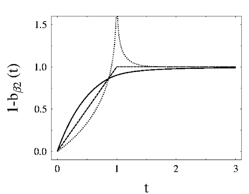
FIG. 10.: Relevant parts $1-b_{\beta 2}(t)$ of the Fourier transforms of the unfolded two–level correlation functions $X_{\beta 2}(r)=1-Y_{\beta 2}(r)$. The functions $b_{\beta 2}(t)$ are referred to as the two–level form factors. The solid line is the GOE result ($\beta=1$), the dashed line is the GUE result ($\beta=2$) and the dotted line is the GSE result ($\beta=4$). The different oscillatory structure of the two–level correlation functions is most strikingly reflected by the behavior of the Fourier transforms at $|t|=1$.

The discontinuities of these functions or there derivatives reflect the different oscillatory structures of the two–level correlation functions. We notice the singularity at $|t|=1$ in $b_{4,2}(t)$.

B Analysis of data and spectral observables

In this section, we review some methods used in the statistical analysis of experimental data, and we summarize the relevant predictions of Random Matrix Theory. The unfolding procedure is described in Sec. III B 1. Then, we discuss several statistical observables: The nearest neighbor spacing distribution (Sec. III B 2), long–range spectral observables (Sec. III B 3), and Fourier transform methods (Sec. III B 4). The superposition of several independent spectra is treated in Sec. III B 5. Specific properties of Random Matrix Theory may yield additional tests of data. In Sec. III B 6, we present the GSE test of GOE data as an example. The predictions of Random Matrix Theory are based on ensemble averages while experimental results are obtained from a running average over the spectrum of a single sample. The justification for this procedure is non–trivial and raises the question of ergodicity. This question is briefly discussed in Sec. III B 7.

1 Unfolding procedure

A measurement or a calculation yields an ordered sequence of energies $\{E_{1},E_{2},\ldots,E_{N}\}$ which form the stick spectrum or spectral function,

$$S(E)=\sum_{n=1}^{N}\delta(E-E_{n})\ .$$ (69)

To analyze the fluctuation properties, this spectrum has to be unfolded, i.e. the system–specific mean level density $R_{1}(E)$ must be removed from the data. We define the cumulative spectral function

$$\eta(E)=\int_{-\infty}^{E}S(E^{\prime})dE^{\prime}=\sum_{n=1}^{N}\Theta(E-E_{n})\ .$$ (70)

This function counts the number of levels with energy less than or

FIG. 11.: Example of an experimentally obtained staircase function. The top figure shows the cumulative spectral function $\eta(E)$ for a spectrum of 1428 elastomechanical eigenfrequencies of a resonating quartz block in the frequency range between 600 kHz and 900 kHz. To keep with the notation in the text, the frequency is denoted by $E$. The inset shows a small section of the measured spectrum between 820 kHz and 825 kHz. Due to the high number of levels, the staircase function appears as a smooth line. The smooth part $\xi(E)$ is a polynomial whose coefficients were found by a fit. The bottom part shows a small section of the staircase function between 699 kHz and 705 kHz, containing about 25 levels. The corresponding section of $\xi(E)$, i.e. the polynomial fit, is drawn as a thin line. We notice that $\xi(E)$ is obtained by fitting to the entire cumulative spectral function, not only to this section. Adapted from Ref. [7].

equal to $E$ and is also referred to as the staircase function. It is decomposed into a smooth part $\xi(E)$ and a fluctuating part $\eta_{\rm fl}(E)$,

$$\eta(E)=\xi(E)+\eta_{\rm fl}(E)\ .$$ (71)

The smooth part is given by the cumulative mean level density,

$$\xi(E)=\int_{-\infty}^{E}R_{1}(E^{\prime})dE^{\prime}\ .$$ (72)

An example for an experimentally obtained staircase function and its smooth part is shown in Fig. 11. To unfold the spectrum, the sequence $\{E_{1},E_{2},\ldots,E_{N}\}$ is mapped onto the numbers $\{\xi_{1},\xi_{2},\ldots,\xi_{N}\}$ with

$$\xi_{n}=\xi(E_{n})\ ,\qquad n=1,\ldots,N\ .$$ (73)

In these new variables the cumulative spectral function simply reads

$$\widehat{\eta}(\xi)=\xi+\widehat{\eta}_{\rm fl}(\xi)\ .$$ (74)

The mean level density of the unfolded spectrum, i.e. the derivative of the smooth part with respect to $\xi$, is unity, as required. Comparing Eqs. (7) and (72) we see that the present unfolding procedure coincides with the analytical unfolding in Random Matrix Theory. Therefore, measurement and theoretical prediction can be directly compared with each other. In practice, the separation in Eq. (71) of a spectrum into a smooth and a fluctuating part can be non–trivial task.

2 Nearest neighbor spacing distribution

The nearest neighbor spacing distribution $p(s)$ is the observable most commonly used to study the short–range fluctuations in the spectrum. This function is equal to the probability density for two neighboring levels $\xi_{n}$ and $\xi_{n+1}$ having the spacing $s$. The function $p(s)$ involves all correlation functions $R_{k}$ with $k\geq 2$ and differs from the two–level correlation function $X_{2}(r)$. The latter gives the probability of finding any two levels at a distance $r$ from each other. Only for small arguments, $p(s)$ is approximated by $X_{2}(s)$. The function $p(s)$ and its first moment are normalized to unity,

$$\int_{0}^{\infty}p(s)ds=1\qquad{\rm and}\qquad\int_{0}^{\infty}sp(s)ds=1\ .$$ (75)

For the uncorrelated or Poisson case, $p(s)=\exp(-s)$ while for the harmonic oscillator, $p(s)=\delta(s-1)$. For the Gaussian ensembles, the analytical calculation of $p(s)$ from the correlation functions given in Sec. III A is possible but highly non–trivial [23]. It leads to expressions involving infinite

FIG. 12.: The Wigner surmises $p_{\beta}(s)$ for the nearest neighbor spacing distribution. The solid line is the result for orthogonal symmetry ($\beta=1$), the dashed line is the result for unitary symmetry ($\beta=2$) and the dotted line is the result for symplectic symmetry ($\beta=4$). We notice the importance of the repulsion law $s^{\beta}$ for small spacings.

products. An excellent approximation is given by the Wigner surmises which are the exact “spacing distribution” for a $2\times 2$ matrix model [63] with Gaussian probability density function. In the most general form the Wigner surmises reads

$$p_{\beta}(s)=a_{\beta}s^{\beta}\exp\left(-b_{\beta}s^{2}\right)$$ (76)

for all three symmetry classes with $\beta=1,2,4$. The level repulsion factor $s^{\beta}$ reflects the Vandermonde determinant in the $N$–level probability density (16). The constants

$$a_{\beta}=2\frac{\Gamma^{\beta+1}((\beta+2)/2)}{\Gamma^{\beta+2}((\beta+1)/2)}\qquad{\rm and}\qquad b_{\beta}=\frac{\Gamma^{2}((\beta+2)/2)}{\Gamma^{2}((\beta+1)/2)}$$ (77)

are explicitly given by $a_{1}=\pi/2$, $b_{1}=\pi/4$ (GOE), $a_{2}=32/\pi^{2}$, $b_{2}=4/\pi$ (GUE), and $a_{4}=262144/729\pi^{3}$, $b_{4}=64/9\pi$ (GSE), respectively. These functions $p_{\beta}(s)$ are shown in Fig. 12. The Gaussian fall–off of $p(s)$ with large $s$ is unrelated to the assumed Gaussian probability density of the three ensembles. Because of universality, the spacing distribution (76) is valid for a wide class of probability densities, see Sec. VIII.

A statistical argument due to Wigner [64] leads to an interesting heuristic formula for the spacing distribution,

$$p(s)=\mu(s)\exp\left(-\int_{0}^{s}\mu(s^{\prime})ds^{\prime}\right)\ .$$ (78)

The repulsion function $\mu(s)$ models the presence or absence of the Vandermonde determinant in the eigenvalue probability density. For a linear repulsion $\mu(s)=\pi s/2$ one obtains the Wigner surmise, for a constant value $\mu(s)=1$, the Poisson distribution. Choosing $\mu(s)=c_{q}s^{q}$ with $0\leq q\leq 1$ leads to the Brody distribution [65],

$$p_{q}(s)=c_{q}s^{q}\exp\left(-\frac{c_{q}}{q+1}s^{q+1}\right)\qquad{\rm with}\qquad c_{q}=\frac{\Gamma^{q+1}(1/(q+1))}{q+1}\ .$$ (79)

In the case of orthogonal symmetry ($\beta=1$), this distribution interpolates between the Poisson case and the Wigner surmise (76). The free parameter $q$ serves as a purely phenomenological measure for the degree of mixing between Poisson and GOE statistics. Izrailev [66, 67] proposed a different phenomenological interpolation formula,

$$p_{\beta_{\rm eff}}(s)=A_{\beta_{\rm eff}}s^{\beta_{\rm eff}}\exp\left(-\frac{\pi^{2}\beta_{\rm eff}}{16}s^{2}-\left(B_{\beta_{\rm eff}}-\frac{\pi\beta_{\rm eff}}{4}\right)s\right)\ .$$ (80)

The parameter $\beta_{\rm eff}$ varies smoothly between zero, the Poisson repulsion factor, and four, which applies to symplectic symmetry. The normalization constants $A_{\beta_{\rm eff}}$ and $B_{\beta_{\rm eff}}$ have to be determined from Eqs. (75). Caurier et al. [68] and Lenz and Haake [69] calculated yet another interpolation formula for the spacing distribution starting from two–dimensional matrix models.

Whenever the agreement of one of the distributions $p(s)$ with data or numerical calculations is tested, it is helpful to use the integral

$$F(s)=\int_{0}^{s}p(s^{\prime})ds^{\prime}$$ (81)

which is referred to as the cumulative spacing distribution.

3 Long–range spectral observables

The nearest neighbor spacing distribution contains information about the spectrum which involves short scales (a few mean level spacings). Long–range correlations are measured by quantities such as the level number variance $\Sigma^{2}(L)$ and the spectral rigidity $\Delta_{3}(L)$. The level number variance is given by

$$\Sigma^{2}(L)=\langle\widehat{\eta}^{2}(L,\xi_{s})\rangle-\langle\widehat{\eta}(L,\xi_{s})\rangle^{2}\ .$$ (82)

Here, $\widehat{\eta}(L,\xi_{s})$ counts the number of levels in the interval [$\xi_{s},\xi_{s}+L$] on the unfolded scale. The angular bracket in Eq. (82) denotes the average over starting points $\xi_{s}$. By construction, i.e. unfolding, one has $\langle\widehat{\eta}(L,\xi_{s})\rangle=L$. Thus, in an interval of length $L$ one expects on average $L\pm\sqrt{\Sigma^{2}(L)}$ levels. The spectral rigidity, introduced by Dyson and Mehta [70], is closely related to $\Sigma^{2}(L)$. In an interval of length $L$. it is defined as the least square deviation of the staircase function $\widehat{\eta}(\xi)$ from the best fit to a straight line,

$$\Delta_{3}(L)=\frac{1}{L}\left\langle\min_{A,B}\int_{\xi_{s}}^{\xi_{s}+L}\left(\widehat{\eta}(\xi)-A\xi-B\right)^{2}d\xi\right\rangle\ .$$ (83)

The angular bracket is defined as in Eq. (82). The definition (83) is very natural since by construction, the smooth part of the staircase function $\widehat{\eta}(\xi)$ is $\xi$ itself. The bottom part of Fig. 11 illustrates the meaning of the spectral rigidity $\Delta_{3}(L)$. Since the few stairs below 702 kHz come quite regularly, there is only a small root–mean–square deviation from the thin line describing the smooth behavior. This implies a small contribution to $\Delta_{3}(L)$. Some of the levels above 702 kHz are nearly degenerate which makes the succession of the stairs rather irregular. Thus, the deviation from the smooth part is larger, yielding a larger contribution to $\Delta_{3}(L)$. We notice that the staircase function in Fig. 11 is shown on the original scale prior to unfolding. However, since the section in the bottom part is small, the smooth part is almost a straight line and the statements just made apply qualitatively also to the unfolded case. For fixed $\xi_{s}$, Bohigas and Giannoni [71, 47] have given a very useful procedure to obtain $\Delta_{3}(L)$ from a measured or calculated spectrum. A proper error analysis for $\Sigma^{2}(L)$ and $\Delta_{3}(L)$ is non–trivial because the results for different values of $L$ are strongly correlated. A consistent method of estimating errors was given by Shriner and Mitchell [72].

In contrast to the spacing distribution, both the number variance and the spectral rigidity probe only two–level correlations. Indeed, $\Sigma^{2}(L)$ can be reduced to the form [47]

$$\Sigma^{2}(L)=L-2\int_{0}^{L}(L-r)Y_{2}(r)dr\ ,$$ (84)

provided the spectrum is translation invariant. As a consequence the number variance is related to the two–level form factor $b_{2}(t)$ defined in Eq. (59),

$$\lim_{L\to\infty}\frac{1}{L}\Sigma^{2}(L)=1-b_{2}(0)\ .$$ (85)

For the Poisson spectrum without correlations and for the harmonic oscillator one obtains $\Sigma^{2}(L)=L$ and $\Sigma^{2}(L)=0$, respectively. The results for the Gaussian ensembles lie between these limiting cases. For large $L$ and $\beta=1,2,4$ one finds the following approximations [70, 23], valid to order $1/L$,

$$\Sigma^{2}_{1}(L) = \frac{2}{\pi^{2}}\left(\ln(2\pi L)+\gamma+1-\frac{\pi^{2}}{8}\right)$$ (86)

$$\Sigma^{2}_{2}(L) = \frac{1}{\pi^{2}}\left(\ln(2\pi L)+\gamma+1\right)$$ (87)

$$\Sigma^{2}_{4}(L) = \frac{1}{2\pi^{2}}\left(\ln(4\pi L)+\gamma+1+\frac{\pi^{2}}{8}\right)\ .$$ (88)

Here $\gamma=0.5772\ldots$ is Euler’s constant. These approximations display the famous logarithmic behavior and the increasing stiffness of the spectrum with increasing $\beta$. Exact expressions can be found, for example in Sec. V C of Ref. [18], they are shown in

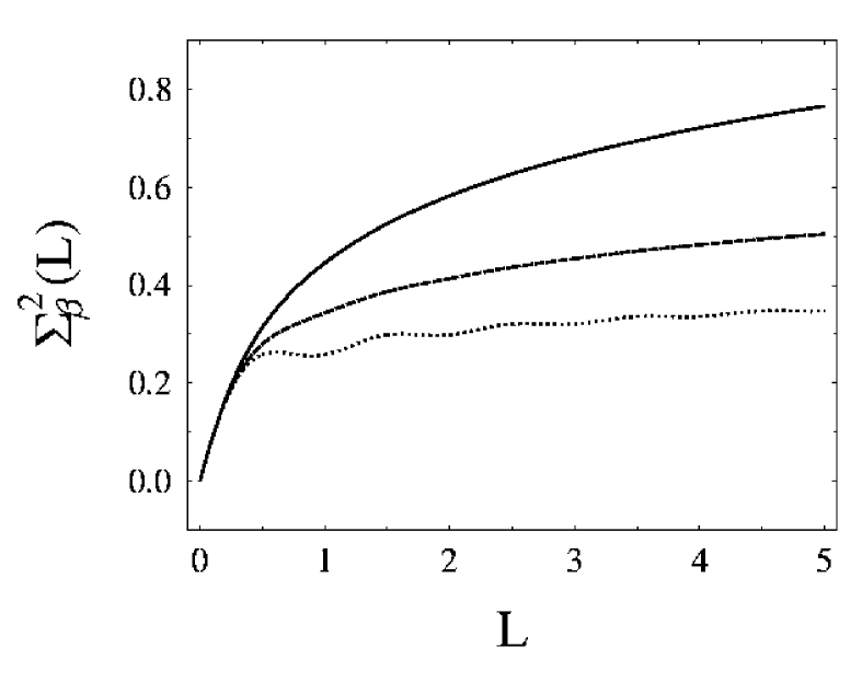
FIG. 13.: The level number variances $\Sigma^{2}_{\beta}(L)$ for the Gaussian ensembles. These are the exact results obtained from the integral (84). The solid line is the GOE result ($\beta=1$), the dashed line is the GUE result ($\beta=2$) and the dotted line is the GSE result ($\beta=4$). We notice the oscillations in $\Sigma^{2}_{4}(L)$ which are not contained in the logarithmic approximation of Eq. (88).

Fig 13. There is a minor misprint in Eq. (5.13) of Ref. [18] for $\Sigma^{2}_{4}(L)$, the argument of $\Sigma^{2}_{2}$ on the right hand side of this equation should read $2r$ instead of $r$. Moreover, we notice that there are visible oscillatory modulations in $\Sigma^{2}_{4}(L)$ which are not borne out in the approximation (88).

The spectral rigidity can similarly be expressed as an integral over the two–point function, and the minimization in Eq. (83) can be done analytically [70, 73, 23]. For a spectrum which is invariant under a continuous set of transformations, one arrives at

$$\Delta_{3}(L)=\frac{L}{15}-\frac{1}{15L^{4}}\int_{0}^{L}(L-r)^{3}(2L^{2}-9Lr-3r^{2})Y_{2}(r)dr$$ (89)

which shows a close formal similarity to Eq. (84). Alternatively, one can write [73]

$$\Delta_{3}(L)=\frac{2}{L^{4}}\int_{0}^{L}(L^{3}-2L^{2}r+r^{3})\Sigma^{2}(r)dr\ .$$ (90)

This equation can be viewed as an integral transform of the level number variance. Remarkably, the parabola is in the kernel of this transform, i.e. inserting $\Sigma^{2}(r)=r^{2}$ yields $\Delta_{3}(L)=0$. For the limiting cases of the Poisson spectrum and the harmonic oscillator, one has $\Delta_{3}(L)=L/15$ and $\Delta_{3}(L)=1/12$, respectively. The results for the Gaussian ensembles can be found by numerical integration. For large $L$ and $\beta=1,2,4$, one has to order $1/L$,

$$\Delta_{3,1}(L) = \frac{1}{\pi^{2}}\left(\ln(2\pi L)+\gamma-\frac{5}{4}-\frac{\pi^{2}}{8}\right)$$ (91)

$$\Delta_{3,2}(L) = \frac{1}{2\pi^{2}}\left(\ln(2\pi L)+\gamma-\frac{5}{4}\right)$$ (92)

$$\Delta_{3,4}(L) = \frac{1}{4\pi^{2}}\left(\ln(4\pi L)+\gamma-\frac{5}{4}+\frac{\pi^{2}}{8}\right)\ .$$ (93)

These approximations show once more the close relation between $\Delta_{3,\beta}(L)$ and the level number variance $\Sigma^{2}_{\beta}(L)$.

We do not address here observables which probe three–level, four–level or even higher–order correlations. We refer the reader to Refs. [70, 47]. In real systems, non–generic and system–specific properties exist which are not described by Random Matrix Theory. These show up on large scales and are discussed in later sections.

4 Fourier transforms

Extracting the positions of the levels from a measured spectrum can be difficult for at least two reasons. Either the resolution is so poor that the extracted sequence is incomplete, or the data set is so large that the task of finding all levels is simply too tedious. In these cases it is desirable to introduce a statistical observable which is directly related to the measured spectrum and in some way separates the statistics of the level positions from the fluctuations due to the line shapes of the levels. The correlation–hole method introduced by Leviandier et al. [74] is a first successful step in this direction.

We consider a measured spectrum $I(\xi)$ on the unfolded scale $\xi$. The observable of interest is the decay function, i.e. the square modulus of the Fourier transform of the spectrum

$$|c(t)|^{2}=\Bigg{|}\int\limits_{-\infty}^{+\infty}d\xi\,I(\xi)\,\exp(2\pi i\xi t)\Bigg{|}^{2}\ .$$ (94)

The Fourier coordinate $t$ defines an unfolded time. Expression (94) can be rewritten as the Fourier transform

$$|c(t)|^{2}=\int\limits_{-\infty}^{+\infty}A(r)\exp(2\pi irt)dr$$ (95)

of the autocorrelation function

$$A(r)=\int\limits_{-\infty}^{+\infty}I(R-r/2)I(R+r/2)dR\ .$$ (96)

This autocorrelation function still contains non–generic information about the system. To obtain the generic statistical properties, $A(r)$ or, equivalently, $|c(t)|^{2}$ have to be smoothed properly [75]. The resulting function $\langle A(r)\rangle$ is generically translation invariant and can be related to the two–level cluster function $Y_{2}(r)$ of Random Matrix Theory. The decay function $|c(t)|^{2}$ is correspondingly related to the two–level form factor $b_{2}(t)$ and at short times reflects long–range spectral correlations, see Eq. (85).

To be definite we discuss the model spectrum

$$I(\xi)=\sum_{n=1}^{N}y_{n}L(\xi-\xi_{n})$$ (97)

studied in Ref. [76] and investigated in a similar form in Refs. [74, 77, 78, 79]. Here, the levels $\xi_{n},\ n=1,\ldots,N$ on the unfolded scale have a common line shape $L(\xi)$ and random intensities $y_{n}$, $N$ is assumed to be a very large number. For non–negative times the decay function is given by [74, 77, 78, 79, 76]

$$|c(t)|^{2}=N\overline{y^{2}}\delta(t)+N\overline{y^{2}}\left(1-\alpha b_{2}(t)\right)|\tilde{L}(t)|^{2}\ ,$$ (98)

with $\alpha=\overline{y}^{2}/\overline{y^{2}}$ the ratio of the first two moments of the intensity distribution. The function $\tilde{L}(t)$ is the Fourier transform of the line shape $L(\xi)$. For a Lorentzian line shape, $|\tilde{L}(t)|^{2}$ reflects the exponential decay of the resonances. If $L(\xi)=\delta(\xi)$ and if all intensities $y_{n}$ are unity, the decay function $|c(t)|^{2}$ equals $1-b_{2}(t)$ for non–zero $t$. For an uncorrelated Poisson spectrum we have $b_{2}(t)=0$ and the decay function is constant. In a correlated spectrum derived from one of the Gaussian ensembles the decay function approaches zero with vanishing $t$. This behavior is referred to as the correlation hole. If the intensities are random numbers, the correlation hole is described by the function $1-\alpha b_{2}(t)$ and does not approach zero. In particular, if the intensity distribution is the Porter–Thomas distribution (see Sec. III E 1), one has $\alpha=1/3$. The $\delta$ function in Eq. (98) occurs since we assumed $N$ to be very large. For a finite number of levels, this contribution will acquire a width, see Refs. [77, 79].

The correlation–hole method separates the statistics of the level positions from that of the intensities and line shapes. This is its main advantage. For realistic spectra, i.e. with inclusion of the line widths, the theory of the correlation hole was worked out in Ref. [77, 80]. There, a scattering model was used. The application of the Fourier transform to statistical spectra is summarized and a qualitative discussion given in Ref. [78]. A short version of the theory of the correlation hole is presented in Appendix A of Ref. [79]. In Ref. [81], the correlation hole is related to its classical analogue, the survival probability.

5 Superposition of independent spectra

We consider a system with a set of good quantum numbers such as spin and parity. In such a system, the Hamiltonian $H$ assumes block–diagonal form, $H={\rm diag}(H_{1},H_{2},\ldots,H_{M})$. So far we have always dealt with the spectrum generated by only one of the sub–blocks $H_{m}$, $m=1,\ldots,M$. Now we consider the superposition of $M$ such spectra. The total level density $R_{1}(E)$ is simply the sum of the $M$ sub–block densities, $R_{1}(E)=\sum_{m=1}^{M}R_{1m}(E)$. We assume that these $M$ densities have roughly the same energy dependence, and that the statistical measures for the $M$ individual spectra are known. How can we calculate the corresponding statistical measures for the total spectrum? For the spacing distribution, the answer is already contained in the seminal article by Rosenzweig and Porter [82] of 1960, see also Mehta’s book [23]. The unfolded observables are expressed in units of the total mean level spacing $D$. Assuming that energy interval of interest is centered around the origin $E=0$, we have $D=1/R_{1}(0)$. We also introduce the fractional densities $g_{m}=R_{1m}(0)/R_{1}(0)$ with $\sum_{m=1}^{M}g_{m}=1$. Let $p_{m}(g_{m}s),\ m=1,\ldots,M$ be the nearest neighbor spacing distribution of the $m$–th sub–spectrum. No assumption is made on the form of the distributions $p_{m}(g_{m}s)$. The spacing distribution $p(s)$ of the superposition of the $M$ spectra is found to be

$$p(s) = \frac{d^{2}}{ds^{2}}E(s)=E(s)\Bigg{(}\sum_{m=1}^{M}g_{m}^{2}\frac{p_{m}(g_{m}s)}{E_{m}(g_{m}s)}+$$ (100)

$$\qquad\left(\sum_{m=1}^{M}g_{m}\frac{1-F_{m}(g_{m}s)}{E_{m}(g_{m}s)}\right)^{2}-\sum_{m=1}^{M}\left(g_{m}\frac{1-F_{m}(g_{m}s)}{E_{m}(g_{m}s)}\right)^{2}\Bigg{)}\ ,$$

where $E(s)=\prod_{m=1}^{M}E_{m}(g_{m}s)$ and

$$F_{m}(g_{m}s)=\int_{0}^{g_{m}s}p_{m}(s^{\prime})ds^{\prime}\ ,\qquad E_{m}(g_{m}s)=\int_{g_{m}s}^{\infty}(1-F_{m}(s^{\prime}))ds^{\prime}\ .$$ (101)

Whenever the long–range spectral observables of interest are pure two–point measures, it is easy to relate those of the full spectrum and those of the $M$ individual spectra. Let $Y_{2m}(g_{m}r)$ be the two–level cluster function, $\Sigma_{m}^{2}(g_{m}L)$ the level number variance, and $\Delta_{3m}(g_{m}L)$ the spectral rigidity of the $m$-th sub–spectrum, respectively. These observables are completely arbitrary. Just like the $p_{m}(g_{m}s)$, they may coincide with but are not restricted to any of the specific forms presented in previous sections. From the definition of the two–point correlation function, one finds immediately for the total two–level cluster function

$$Y_{2}(r)=\sum_{m=1}^{M}g_{m}^{2}Y_{2m}(g_{m}r)\ .$$ (102)

It then follows directly from Eqs. (84), (89) and (90) that

$$\Sigma^{2}(L)=\sum_{m=1}^{M}\Sigma_{m}^{2}(g_{m}L)\qquad{\rm and}\qquad\Delta_{3}(L)=\sum_{m=1}^{M}\Delta_{3m}(g_{m}L)\ .$$ (103)

The first property (103) is not surprising because $\Sigma^{2}(L)$ is a variance. All results given here apply only to $M$ strictly non–interacting spectra. Crossover transitions due to the breaking of a quantum number are discussed later.

Very important for the analysis of data is the superposition of a large number $M$ of spectra. For all individual distributions $p_{m}(g_{m}s)$ which play a role in realistic spectra the superposition $p(s)$ tends rather quickly towards the Poisson limit. The superposition of only six or so spectra which individually follow the Wigner surmises yields a spacing

FIG. 14.: Nearest neighbor spacing distribution $p(s)$ as given in Eq. (100) for the superposition of $M$ spectra with equal fractional densities $g_{m}=1/M,\ m=1,\ldots,M$. Each individual spectrum follows the Wigner surmise. One has $p(0)=1-1/M$ at $s=0$. The cases $M=2,4,8$ are shown as solid lines. The Wigner surmise and the Poisson distribution are drawn as dashed lines.

distribution which is experimentally hard to distinguish from a Poisson distribution. This is illustrated in Fig. 14 for spectra with equal fractional densities $g_{m}=1/M,\ m=1,\ldots,M$. In this case, formula (100) implies $p(0)=1-1/M$, reflecting the increasing number of degeneracies. For the interval lengths $L$ which are usually available for the analysis of data, a similar statement applies to $\Sigma^{2}(L)$ and $\Delta_{3}(L)$ as superpositions of the relevant individual distributions $\Sigma_{m}^{2}(g_{m}L)$ and $\Delta_{3m}(g_{m}L)$. There are of course exceptions such as, for example, the superposition of pure harmonic oscillator spectra.

The property (102) of the two–level cluster function can be used to estimate the number $M$ of superimposed independent spectra, i.e. of symmetries in a measured spectrum. This is important in situations where an assignment of the set of quantum numbers to every individual level in the spectrum is impossible or too tedious. In a molecular physics context, Leviandier et al. [74] argued that the decay function $|c(t)|^{2}$ introduced in Sec. III B 4 is rescaled by a factor $1/M$ so that the correlation hole becomes narrower by a factor $M$. In a more general discussion [77], a superposition of $M$ independent spectra was considered. Each spectrum has a line shape $L_{m}(\xi)$ and a set of intensities with first and second moments $\overline{y_{m}}$ and $\overline{y_{m}^{2}}$. One finds

$$|c(t)|^{2}=f_{0}\delta(t)+f_{1}\sum_{m=1}^{M}g_{m}\overline{y_{m}^{2}}\left(1-\alpha_{m}b_{2}(t/g_{m})\right)|\tilde{L}_{m}(t)|^{2}$$ (104)

where $f_{0}$ and $f_{1}$ are system–specific constants, and where $\alpha_{m}=\overline{y_{m}}^{2}/\overline{y_{m}^{2}}$. If all $M$ mean level densities $R_{1m}(E)$ are roughly equal, one has $g_{m}\simeq 1/M$, and the correlation hole is indeed narrowed by a factor $M$.

Finally, we mention that Berry and Robnik proposed a spacing distribution supposed to describe the transition from Poisson behavior to the Wigner surmise. This distribution is obtained from formula (100) by taking $M=2$ spectra, one satisfying the Poisson spacing distribution, the other one, the Wigner surmise. Strictly speaking this formula is only applicable to two non–interacting spectra. It is nonetheless often used as a phenomenological guess for mixed systems.

6 GSE test of GOE data

We consider a GOE spectrum $\{E_{1},E_{2},E_{3},...\}$ with $E_{n}\leq E_{n+1}$. We divide the sequence $\{E_{1},E_{2},E_{3},...\}$ into two sequences with odd and even indices, i.e. into $\{E_{1},E_{3},E_{5},...\}$ and $\{E_{2},E_{4},E_{6},...\}$ and consider each as a new spectrum. Then, a theorem due to Mehta and Dyson [83] states that after proper unfolding, each of the two spectra obeys GSE statistics. This theorem was recently used by Lombardi, Bohigas and Seligman [84] for a GSE test of GOE data. In this test, the two–level form factor $b_{2}(t)$ and the correlation hole $|c(t)|^{2}$ are particularly useful observables. In contrast to the GOE case, the GSE form factor has a singularity at $t=1$ caused by the oscillatory structure of the two–level cluster function $Y_{2}(r)$. Thus, one expects a characteristic peak at $|t|=1$ which gives information on correlations on the scale of about two mean level spacings. As pointed out in Ref. [84], the two–level observables calculated for the two subsequences contain information on higher level correlations ($k>2$) of the original spectrum.

7 Ergodicity

In Random Matrix Theory, observables are calculated by averaging over an ensemble of Hamiltonians. This average is indicated by a bar. Experimentally, the observables are calculated as running averages over part of the spectrum of a given system, containing $N_{I}$ levels in the interval $[E,I+E]$. This average is indicated by an angular bracket. For any function $F(E)$ of energy $E$, it is given by

$$\langle F(E)\rangle_{I}=\frac{1}{I}\int_{E}^{E+I}F(E^{\prime})dE^{\prime}=\frac{1}{N_{I}}\int_{0}^{N_{I}}F(E+Dr)dr=\langle F\rangle_{N_{I}}$$ (105)

where $D$ denotes the mean level spacing. A comparison of the results of both procedures is meaningful only if they are equivalent, i.e. if

$$\overline{F(E)}=\langle F(E)\rangle$$ (106)

In this case, one speaks of ergodicity. Mathematical discussions of ergodicity can be rather involved. Here, we only summarize a very instructive discussion by French, Mello and Pandey [85]. It is assumed that the spectrum is generic so that after proper unfolding averaging will give translation invariant results. As a test of ergodicity, French et al. consider the variance

$${\rm var}\langle F\rangle_{N_{I}}=\overline{|\langle F-\overline{F}\rangle|^{2}}\ .$$ (107)

This quantity is the ensemble average of the squared difference between running and ensemble average. It can be cast into a form similar to Eq. (84) for the level number variance,

$${\rm var}\langle F\rangle_{N_{I}}=\frac{1}{I^{2}}\int_{-I}^{+I}(I-|\varepsilon|)C_{F}(\varepsilon)d\varepsilon=\frac{1}{N_{I}^{2}}\int_{-N_{I}}^{+N_{I}}(N_{I}-|r|)C_{F}(Dr)dr\ .$$ (108)

The auto-covariance function $C_{F}(\varepsilon)=\overline{(F^{*}(E)-\overline{F}^{*})(F(E+\varepsilon)-\overline{F})}$ is, after proper unfolding, a translation invariant two–point function independent of $E$. With the help of a result of the theory of random functions [86], Eq. (108) leads to

$$\lim_{r\to\infty}C_{F}(Dr)=0\qquad\Longrightarrow\qquad\lim_{N_{I}\to\infty}{\rm var}\langle F\rangle_{N_{I}}=0\ .$$ (109)

or equivalently

$$\lim_{r\to\infty}C_{F}(Dr)=0\qquad\Longrightarrow\qquad\lim_{N_{I}\to\infty}\langle F\rangle_{N_{I}}=\overline{F}\ .$$ (110)

This is the desired ergodic behavior for almost all members of the ensemble, except for a set of measure zero. We note that ergodicity is attained only for a large, preferably infinite, number $N_{I}$ of levels. The result (109) can be generalized fairly easily: The $k$–point function is ergodic if in the limit of infinite energy differences. the ensemble–averaged $2k$–point function vanishes. We have made no specific assumptions concerning $F(E)$. Thus, the argument just presented also applies to correlations of scattering matrix elements and all other level correlators of Random Matrix Theory.

C Introduction to supersymmetry

The description of all technical aspects of supersymmetry would be far beyond the scope of this review. We attempt to give the interested reader an idea of the main elements of the method. For further reading, we mention Berezin’s book [87] where mathematical aspects of superanalysis are described, see also Ref. [88]. Several papers and review articles explain the use of the standard supersymmetry method in problems of chaos and disorder [44, 46, 89, 90], and Efetov [45] has recently devoted a book to the subject. The term “supersymmetry” was first introduced by Wess and Zumino in relativistic field theory [91]. In the present context, supersymmetry does involve a symmetry between bosonic and fermionic integration variables but lacks the invariance properties of a relativistic field theory. Perhaps more importantly, the fermionic variables lack any physical meaning and are introduced merely as bookkeeping devices. Wherever applicable, the supersymmetry method has been found to be more powerful than the replica trick: It yields exact results where the replica trick only yields asymptotic expansions. The price one has to pay consists in using analysis on supermanifolds. The replica trick, on the other hand, finds a much wider range of applications.

In Sec. III C 1 we derive the supersymmetric representation of the generating function for level correlators. In Sec. III C 2, the saddle–point approximation is used to derive the standard supersymmetric non–linear $\sigma$ model. An alternative technique which avoids the saddle–point approximation and is useful for purely spectral observables is discussed in Sec. III F 2.

1 Supersymmetric representation of the generating function

We develop the method for an observable given by the product of the retarded and advanced propagators tr$(E_{1}^{+}-H)^{-1}$ and tr$(E_{2}^{-}-H)^{-1}$, with $H$ a member of the GUE, and $E_{p}^{\pm}=E_{p}\pm i\eta$ with $\eta$ positive infinitesimal and $p=1,2$. It is highly non–trivial to average a product of propagators over an ensemble of matrices $H$ since $H$ appears in the denominators. In Sec. III A, we have shown that the Mehta–Dyson method accomplishes this goal very elegantly in the case of spectral correlations in the pure cases. If, however, an additional matrix $\gamma$ appears in the propagator, rotation invariance in Hilbert space is broken, and almost all of the convenient features of the Mehta–Dyson method disappear. Scattering systems require such an addition to the Hamiltonian to describe the coupling to the channels, see Sec. III D. Prior to the advent of supersymmetry, one was restricted to perturbative or asymptotic expansions in these situations, see Refs. [18, 25].

To keep the presentation transparent, we do not discuss scattering systems and restrict ourselves to the spectral two–point correlation function, even though in this particular case, the supersymmetry method only reproduces the results obtained earlier by Dyson and Mehta. We emphasize again that the supersymmetry method develops its full power in those cases where the Mehta–Dyson method does not apply. Later, we indicate the modifications for other cases (more than two propagators, different symmetry of $H$, propagators in higher dimension). Our choice of observable is dictated by the fact that the occurrence of a pair of complex conjugate propagators is typical of many problems. Our notation is that of Ref. [46]. We use the form $\lambda^{2}/N$ for the variance of the Gaussian distribution of $H$, see Sec. III A 2.

To perform the ensemble average exactly, i.e. non–perturbatively, one expresses the propagator as the derivative of a generating function $F_{p}(J_{p})$ with respect to a source variable $J_{p}$ such that

$${\rm tr}\frac{1}{E_{p}^{\pm}-H}=\frac{\partial}{\partial J_{p}}F_{p}(J_{p})\Bigg{|}_{J_{p}=0}\ .$$ (111)

It is easily seen that the choice

$$F_{p}(J_{p})=\frac{{\rm det}(E_{p}^{\pm}-H+J_{p})}{{\rm det}(E_{p}^{\pm}-H-J_{p})}$$ (112)

represents such a generating function. We observe that the logarithms of the numerator and the denominator separately generate the propagator, too. In contrast to the latter, however, the function $F_{p}(J_{p})$ has the very useful property of being normalized to unity, i.e. to a constant independent of $H$: We have $F_{p}(0)=1$. Still, an exact average of $F_{p}(J_{p})$ over the ensemble seems out of question. This is the point where supersymmetry enters. The inverse of an $N\times N$ determinant can be expressed as the Gaussian integral over an $N$ component vector $S_{p}$ of complex commuting variables, while the determinant itself is given as the Gaussian integral over an $N$ component vector $\chi_{p}$ of complex anticommuting variables. Thus we have

$$F_{p}(J_{p}) = \int d[S_{p}]\exp\left(iS_{p}^{\dagger}(E_{p}^{\pm}-H-J_{p})S_{p}\right)$$ (114)

$$\qquad\int d[\chi_{p}]\exp\left(i\chi_{p}^{\dagger}(E_{p}^{\pm}-H+J_{p})\chi_{p}\right)\ .$$

Calculating the average over the Gaussian ensemble is now straightforward since $H$ appears in the exponent.

With these tools, we can derive the generating function of the two–point function. It is convenient to write $E=(E_{1}+E_{2})/2$ and $\varepsilon=E_{1}-E_{2}$. To be consistent with most of the literature, we use the symbol $\varepsilon$ throughout this section and the symbol $\omega$ in its stead in Sec. VI. We already know that the unfolded two–point function will only depend on $\varepsilon/D$ where $D$ is the mean level spacing. We have to take into account that the imaginary increment $i\eta$ lies on different sides of the real axis for $p=1$ and $p=2$. To ensure convergence of the integrals one proceeds as follows. We define a metric $L={\rm diag}(+1,+1,-1,-1)$, reflecting the location of $i\eta$, and the direct product ${\bf L}=L\otimes 1_{N}$. Here, $1_{N}$ denotes the $N\times N$ unit matrix. Moreover we set $J={\rm diag}(-J_{1},+J_{1},-J_{2},+J_{2})$ and introduce the supervector $\Psi=(S_{1},\chi_{1},S_{2},\chi_{2})^{T}$. The proper generating function is then given by

$$F_{1}(J_{1})F_{2}(J_{2}) = \int d[\Psi]\exp\biggl{(}i\Psi^{\dagger}{\bf L}^{1/2}\biggl{(}1_{4}\otimes(E-H)$$ (116)

$$\qquad\qquad+\left(\frac{\varepsilon}{2}+i\eta\right)L\otimes 1_{N}+J\otimes 1_{N}\biggl{)}{\bf L}^{1/2}\Psi\biggl{)}\ .$$

Some authors prefer a different form for expression (116): The symmetric arrangement of the two factors $L^{1/2}$ is dropped in favor of a single factor $L$ appearing right behind $\Psi^{\dagger}$.

For an observable containing $k>2$ propagators (usually an equal number of advanced and of retarded propagators), the form of Eq. (116) would be the same, but the dimension of the vectors $\Psi$ and of the supermatrices would be $2kN$ rather than $4N$. The dimensions of the supermatrices and supervectors and their internal symmetries would change for real symmetric or quaternion (rather than Hermitean) matrices $H$. The “source term” $J\otimes 1_{N}$ must be altered, if matrix elements (rather than traces) of the propagators are considered. For Hamiltonians in $d>0$ dimensions, the four–component super vectors $\Psi_{n}^{\dagger}$ and $\Psi_{n}$ with $n=1,\ldots,N$ are replaced by space–dependent vectors $\Psi(\vec{r})^{\dagger}$ and $\Psi(\vec{r})$, respectively, and the bilinear forms in the matrix space of $H$ are replaced by integrations over $d$–dimensional space. The generating function becomes a generating functional, and the theory turns into a field theory.

Only the $H$–dependent term in expression (116) is affected by averaging over the GUE. It is easy to calculate

$$\int d[H]P_{N2}(H)\exp\left(-i\Psi^{\dagger}(L\otimes H)\Psi\right)=\exp\left(\frac{1}{2N}{\rm trg}A^{2}\right)$$ (117)

where

$$A=i\lambda L^{1/2}\sum_{n=1}^{N}\Psi_{n}\Psi_{n}^{\dagger}L^{1/2}$$ (118)

is a four by four supermatrix. The symbol ${\rm trg}$ denotes the supertrace. The term ${\rm trg}A^{2}$ in the exponent is of fourth order in the integration variables contained in $\Psi_{n}$, and a direct integration over these variables is, therefore, impossible. This difficulty is overcome with the help of the Hubbard–Stratonovich transformation. The fourth–order term in the exponent is reduced to second order at the expense of introducing a set of auxiliary integration variables,

$$\exp\left(\frac{1}{2N}{\rm trg}A^{2}\right)=\int d[\sigma]\exp\left(-\frac{N}{2}{\rm trg}(\sigma^{2})-{\rm trg}(\sigma A)\right).$$ (119)

The matrix $\sigma$ has essentially the same symmetries as the matrix $iA$. The differential $d[\sigma]$ denotes the product of the differentials of the independent matrix elements. The integration over the $\Psi_{n}$ can now be done. The procedure sketched in Eqs. (117) and (119) can also be viewed as a double Fourier transform, the first in ordinary, the second in superspace [92].

Collecting everything, we find for the ensemble average $\overline{F_{1}(J_{1})F_{2}(J_{2})}$ of the generating function (116)

$$\overline{F_{1}(J_{1})F_{2}(J_{2})}=\int d[\sigma]\exp{\cal L}(\sigma)$$ (120)

where the “Lagrangean” ${\cal L}$ has the form

$${\cal L}(\sigma)=-\frac{N}{2}\ {\rm trg}(\sigma^{2})-N\ {\rm trg}\ln\left(E1_{4}-\lambda\sigma+J+\frac{\varepsilon}{2}L\right).$$ (121)

In the case of a disordered system which might, for instance, be described by a single–particle Hamiltonian $H=T+V$ where $T$ is the kinetic energy operator, and $V$ is an impurity potential of the form (14), one obtains similarly a generating functional where $\sigma$ is a function of ${\vec{r}}$, and where the operator $T$ appears as argument under the logarithm.

Equations (120,121) embody the first important result of the supersymmetry technique: The ensemble average of $F_{1}(J_{1})F_{2}(J_{2})$ has been calculated, and the resulting integral expressed in terms of a small number of integration variables, determined by the number of independent elements in the matrix $\sigma$. The $4N$ original complex integration variables $\Psi$ have disappeared.

The matrix $\sigma$ possesses the same dimension and the same symmetries as the matrix $iA$. The matrix $iA$, in turn, comprises all the unitary invariants which can be constructed from the elements of each, equivalent, vector $\Psi_{n}$. Only such invariants survive the ensemble average. Hence, both $iA$ and $\sigma$ directly mirror the underlying unitary symmetry in superspace. Moreover, the dimension of ${\sigma}$ is as small as is consistent with both the form of the observable, and the symmetry of the problem.

These statements apply equally to observables involving $k$–point functions, see for example Ref. [92], and to problems with orthogonal [46] or symplectic symmetry. For Hamiltonians in $d\geq 1$ dimensions, the matrix $\sigma$ attains a dependence on a spatial variable $\vec{r}$. With proper modifications, the statements just made carry over to this case, too, and the resulting expression for the generating functional constitutes a genuine field theory [44]. In a conceptually important work, Zirnbauer [93] recently extended the supersymmetry method to to the circular ensembles, i.e. to systems with unitary disorder.

2 Saddle–point approximation and non–linear $\sigma$ model

The second important step of the supersymmetry technique consists in an approximate evaluation of the remaining integrations in the ensemble–averaged supersymmetric generating function in Eqs. (120,121), or at least in the reduction of the problem to a non–linear $\sigma$ model. This is accomplished by using the saddle–point approximation, suggested by the occurrence of the factor $N$ multiplying all terms in the exponent. We recall that in RMT, we always take the limit $N\rightarrow\infty$. In some cases, it is advantageous to avoid the saddle–point approximation, and to use an alternative technique, see Sec. III F.

The generating function (120,121) possesses an important symmetry: Except for its dependence on $J$ and $\varepsilon$, it remains invariant under the group $G$ of those global transformations $T$ with $\sigma\rightarrow T^{-1}\sigma T$ which do not change the symmetry of $\sigma$. The form of the supermatrices $T$ which fulfill this requirement depends, of course, on the dimension of the matrix $\sigma$ and on the symmetry (orthogonal, unitary or symplectic) of the underlying Hamiltonian ensemble.

The saddle point is found after neglecting in the expression (121) for ${\cal L}$ both the term $\varepsilon$ and the source term $J$. This is justified since $\varepsilon$ scales with $1/N$. Indeed, the fluctuations depend on the unfolded energy difference $\varepsilon/D$. Since $D$ vanishes like $1/N$, the same must be true for $\varepsilon$. The source term $J$ may be viewed as being infinitesimally small since the derivatives with respect to $J$ are taken at $J=0$. The saddle–point equation is

$$\sigma=\frac{\lambda 1_{4}}{E-\lambda\sigma}.$$ (122)

This matrix equation is solved in two steps. First, a diagonal matrix $Q_{0}$ is found which obeys Eq (122). For $|E|\leq 2\lambda$, i.e. if $E$ lies within Wigner’s semicircle, the elements $Q^{\pm}$ of $Q_{0}$ have the values $Q^{\pm}=E/(2\lambda)\pm i\sqrt{1-(E/(2\lambda))^{2}}$. For a two–point function, i.e. a product of the trace of an advanced and of a retarded propagator, it is necessary to choose $Q_{0}=$ diag$(Q^{+},Q^{+},Q^{-},Q^{-})$.

This choice breaks the symmetry under the group $G$ defined above. This is most easily seen by writing $Q_{0}$ in the form

$$Q_{0}=\frac{E}{2\lambda}1_{4}+\frac{\pi\lambda\rho(E)}{N}L$$ (123)

with $\rho$ defined in Eq. (7). The matrix $L$ does not commute with all elements $T$ of $G$: The symmetry is broken by the mean level density $\rho$. We will see shortly that as a consequence of this broken symmetry, there occurs a Goldstone or zero mode.

All matrices $Q=T^{-1}Q_{0}T$ obtained from $Q_{0}$ by application of a transformation $T\in G$ are also solutions of the saddle–point equation, and the totality of all these matrices defines the saddle–point manifold. Let $G_{R}$ with elements $R$ be the maximum subgroup of $G$ which obeys $[R,L]=0$ for all $R\in G_{R}$. This subgroup leaves $Q_{0}$ invariant. Let $G/G_{R}$ be the associated coset space with elements $T_{0}$. Every $T\in G$ can be written in the form $T=RT_{0}$ with $R\in G_{R}$ and $T_{0}\in G/G_{R}$. The saddle–point manifold is then given by $Q=T_{0}^{-1}Q_{0}T_{0}$. This manifold has dimension $d>0$ precisely because the symmetry under $G$ is broken by $Q_{0}$, and it therefore constitutes the Goldstone mode caused by the broken symmetry.

In a seminal paper, Schäfer and Wegner [39] investigated the structure of the saddle–point manifold for bosonic variables. In Refs. [44, 46], their work was extended to the supersymmetry formalism. It turns out that the saddle–point manifold possesses mixed (hyperbolic and compact) symmetry. This property of the saddle–point manifold is not reproduced in the replica trick, and is the cause of its failure to produce exact results [36].

The integration over the massive modes (i.e. in directions orthogonal to the saddle–point manifold) can be carried out. For Gaussian RMT, these modes have a mass proportional to $N$, and yield corrections to the saddle–point integral which vanish for $N\rightarrow\infty$. The remaining integrations extend over the coset space $G/G_{R}$ and yield a zero–dimensional non–linear $\sigma$ model (because the saddle–point solutions $Q$ obey the non–linear Eq. (122)). The generating function attains the form

$$\overline{F_{1}(J_{1})F_{2}(J_{2})}=\int d\mu(t)(...)\exp\left(i\frac{\pi\varepsilon}{4D}\ {\rm trg}(QL)\right).$$ (124)

The dots indicate the $J$–dependent terms. Notice that the mean level spacing is given by $D=\pi\lambda/N$ at $E=0$. The integration measure $d\mu(t)$ is defined in terms of a suitable parameterization of the elements $T_{0}$ of the coset space $G/G_{R}$.

Mutatis mutandis, these arguments carry over to the case of disordered solids in $d\geq 1$ dimensions. For the potential model of Eq. (14), the large parameter which formally corresponds to $N$ is $k_{F}l$ where $l=v_{F}\tau$ is the elastic mean free path, $\tau$ is the elastic mean free time, and $k_{F}$ ($v_{F}$) is the Fermi wave number (the Fermi velocity, respectively). The need to use this parameter shows that the supersymmetry technique is confined to problems with weak disorder.

Minimization of the Lagrangean in $d\geq 1$ leads to a diagonal saddle–point solution $Q_{0}$ which has the same form as in RMT. The saddle–point manifold now comprises matrices $Q({\vec{r}})=T_{0}^{-1}({\vec{r}})Q_{0}T_{0}({\vec{r}})$ with a very slow ${\vec{r}}$–dependence (long wave–length limit). The resulting generating functional $\overline{F(Q)}$ has the form

$$\overline{F(Q)} = \int d\mu(t({\vec{r}}))(...)\exp\biggl{(}\frac{\pi\nu}{8}\int d^{d}r\biggl{(}\hbar\ {\cal D}\ {\rm trg}\left(\nabla Q({\vec{r}})\right)^{2}$$ (126)

$$\qquad\qquad\qquad+2i\varepsilon\ {\rm trg}(QL)\biggl{)}\biggl{)}.$$

Here, ${\cal D}=v_{F}^{2}\tau/d$ is the diffusion constant. Except for the additional space dependence, all other symbols have the same meaning as in Eq. (124).

It is instructive to compare the terms in the exponents of Eqs. (124,126). If we disregard the additional space dependence in Eq. (126), the “symmetry–breaking term” proportional to $\varepsilon$ is identical in both cases. Indeed, the space integration yields a factor $V$, so that $\nu V=\Delta^{-1}$, and we surely must identify $\Delta$ with the Gaussian RMT mean level spacing $D=\pi\lambda/N$. The gradient term in Eq. (126) (obviously missing in Eq. (124)) has roughly the magnitude $\hbar{\cal D}/L^{2}=E_{C}$. For $E_{C}<\varepsilon$, this term is more important than the symmetry–breaking term, and conversely, see Sec. VI.

We distinguish a diffusive regime, defined by the condition $g\gg 1$, or $L\ll\xi$ with $\xi$ the localization length, and a localized regime, where $L\gg\xi$. Since $g=E_{C}/\Delta=\xi/L$ in the diffusive regime, see Eq. (17), the conditions $L\ll\xi$ and $E_{C}\gg\Delta$ are equivalent. In the diffusive regime, the symmetry–breaking term is the dominant zero mode. This implies that all correlation functions of the disordered solid are approximately of Gaussian RMT type in this regime! This statement holds for energy differences $|\varepsilon|<E_{C}$ and establishes the close link between Gaussian RMT and localization theory, see Sec. VI. In the localized regime, on the other hand, the gradient term is the dominant zero mode. It may be surprising that in this regime, Eq. (126) retains its validity. The reason is that the characteristic length scale $L_{0}$ over which $Q({\vec{r}})$ varies must obey the inequality $l\ll L_{0}\ll\xi$. This is why a non–linear $\sigma$ model does not apply for $d=1$ where $l=\xi$.

In concluding this introduction to supersymmetry, we notice that the supersymmetric representation of the generating function for the RMT correlators provides an exact re–formulation of the RMT problem. Therefore, all results derived from this function are fully equivalent to the results of classical RMT. Starting from a white–noise potential, on the other hand, one obtains a supersymmetric non–linear $\sigma$ model. In the zero–dimensional limit, this model is fully equivalent to th limit $N\to\infty$ of the supersymmetric representation of RMT. However, the supersymmetry method continues yielding new results which, in many cases, could not be obtained with other techniques.

D Scattering systems

Scattering systems play a very important role in the application of Random Matrix Theory, particularly in the context of transport phenomena in mesoscopic systems. The theory of these systems requires a generalization of the concepts introduced so far for bounded systems and the associated spectral fluctuations. We keep our presentation brief since various well written papers and reviews are available. We mention the early reviews by Eckhardt [94, 95] and Smilansky [96, 97] which contain discussions of chaotic scattering, especially from a semiclassical point of view. Likewise, Doron, Smilansky and Frenkel [98] mainly focus on semiclassical aspects, while Lewenkopf and Weidenmüller [99] concentrate on aspects of Random Matrix Theory and on the comparison with semiclassical results. Very recently, a review of chaotic scattering was presented by Jung and Seligman [100], and one on scattering and transport in mesoscopic and disordered systems by Beenakker [101]. In Sec. III D 1, we summarize general aspects of scattering theory, before we establish the link to Random Matrix Theories in Sec. III D 2.

1 General aspects

In the context of RMT, scattering processes are important in both, cavities and/or mesoscopic wires connected to the outside world by leads or antennae, and non–relativistic many–body systems as encountered in nuclear, atomic and molecular physics. In all these cases, the participants in the scattering process move freely at asymptotically large distances but encounter strong interactions in the interaction region. We idealize a scattering system as consisting of a compact interaction region, i.e. a region of finite volume, and of channels through which this region is accessible and in which the propagation is free. A general scattering theory based on this idealization was constructed by Wigner and Eisenbud [102]. These authors made the physically well justified further assumption that only two–body fragmentation is allowed at low energies. They also postulated short–range interactions. However, the formalism can be extended to the Coulomb interaction, too.

To illuminate the physical content of this approach, we first consider a bound–state problem defined by restricting the motion of all particles to the compact interaction region. Then, the spectrum is discrete. As we allow for the coupling to the channels, many of the bound eigenstates turn into resonances. These resonances may dominate the scattering process. Following Ref. [27], we present here a variant of the general theory which focuses attention from the outset onto such resonances. We consider $N$ orthonormal functions $\varphi_{\mu},\ \mu=1,\ldots,N$ localized on the interaction region, where eventually the limit $N\to\infty$ has to be taken. These functions represent a basis for the quasibound eigenstates. The $\Lambda$ channels are represented by the channel wave functions $\chi_{c}(E),c=1,\ldots,\Lambda$ where $E$ is the total energy. These states obey the orthonormality condition $\langle\chi_{a}(E)|\chi_{b}(E^{\prime})\rangle=\delta_{ab}\delta(E-E^{\prime})$. They do not vanish in the interaction region but are orthogonal to the bound–state wave functions, $\langle\chi_{a}(E)|\varphi_{\mu}\rangle=0$ for all $E,a,\mu$. In this basis, the total Hamiltonian has the form

$${\cal H} = \sum_{\mu,\nu=1}^{N}|\varphi_{\mu}\rangle H_{\mu\nu}\langle\varphi_{\nu}|$$ (129)

$$\qquad+\sum_{\mu=0}^{N}\sum_{c=1}^{\Lambda}\int_{\varepsilon_{c}}^{\infty}dE\left(|\chi_{c}(E)\rangle W_{c\mu}\langle\varphi_{\mu}|+|\varphi_{\mu}\rangle W_{\mu c}\langle\chi_{c}(E)|\right)$$

$$\qquad+\sum_{c=1}^{\Lambda}\int_{\varepsilon_{c}}^{\infty}dE|\chi_{c}(E)\rangle E\langle\chi_{c}(E)|\ .$$

Here $\varepsilon_{c}$ is the threshold energy in channel $c$ (for $E<\varepsilon_{c}$ only evanescent waves exist, and for $E>\varepsilon_{c}$ the channel is said to be open). The first term in Eq. (129) involves the $N\times N$ matrix $H$ which describes the mutual coupling of the bound states. The second term contains the $N\times\Lambda$ coupling matrix $W$ between channels and bound states. This term causes the bound states to acquire widths, and to become resonances. The third term is assumed to be diagonal in the channels. This assumption can be lifted but provides a useful simplification and is realistic in later applications. In the framework of Eq. (129), transitions between different channels are possible only via intermediate population of the bound states. We assume that elastic background phase shifts in the channels can be neglected so that the functions $\chi_{a}(E)$ are essentially plane waves.

The physical assumptions made in this model become even more transparent as one works out [27] the scattering matrix $S_{ab}(E)$,

$$S_{ab}(E)=\delta_{ab}-i2\pi W_{a}^{\dagger}D^{-1}(E)W_{b}$$ (130)

where the $N$ component vector $W_{a}$ is the $a$–th column of the matrix $W$. The propagator $D^{-1}(E)$ is the inverse of

$$D(E)=E1_{N}-H+i\pi\sum_{c\ {\rm open}}W_{c}W_{c}^{\dagger}\ .$$ (131)

This notation should not be confused with that for the mean level spacing $D$ between the eigenvalues of $H$. All threshold effects, including the dependence of $W$ on $E$ have been neglected. The scattering matrix element $S_{ab}(E)$ has $N$ poles corresponding to $N$ resonances. For $N=1$, the scattering matrix has Breit–Wigner form, with $W_{c1}$ denoting the partial width amplitude. For $N>1$, Eqs. (130) and (131) constitute $N$–level unitary generalizations of the Breit–Wigner formula. In the limit $\sum_{c=1}^{\Lambda}|W_{\mu c}|^{2}\ll D$ for all $\mu$, the model describes $N$ isolated resonances $\mu=1,\ldots,N$, with widths very small compared to the spacing between resonances. Here, $D$ denotes the mean level spacing. As the ratios $\sum_{c=1}^{\Lambda}|W_{\mu c}|^{2}/D$ increase, the resonances begin to overlap. Eventually, one arrives at the Ericson regime of strongly overlapping resonances where the fluctuations of the cross section are no longer related to individual resonances. Increasing the ratios $\sum_{c=1}^{\Lambda}|W_{\mu c}|^{2}/D$ even further, one returns to the regime of isolated resonances.

2 Scattering and Random Matrix Theory

Apart from the general constraints mentioned above, no specific assumptions on the bound–state Hamiltonian $H$ have been made in the derivation of the formal result (130). We now connect this model to RMT by assuming that the Hamiltonian $H$ in the interaction region can be represented by a random matrix drawn from one of the Gaussian ensembles. In particular, for a time–reversal invariant system, $H$ is a member of the GOE. With this assumption, the fluctuation properties of $S$ can be predicted, given the ensemble average of $S$ which serves as an input parameter.

Anticipating the discussion in later sections, we argue that this choice for $H$ is justified in three typical physical situations: Scattering at complex many–body systems, chaotic scattering in few–degrees–of–freedom systems, and scattering by a disordered quantum dot. Indeed, the spectral fluctuation properties of a wide class of complex many–body systems such as nuclei, atoms and molecules are known to be well described by the spectral observables discussed in Sec. III B. Therefore, it is very natural to choose $H$ from the GOE. For chaotic systems with few degrees of freedom, such as billiards, the justification is based on the Bohigas conjecture. For a disordered quantum dot, the random Hamiltonian directly simulates the effect of the random potential.

The autocorrelation function of the scattering matrix $S$ is defined as an ensemble average,

$$C_{abcd}(\varepsilon)=\overline{S_{ab}(E)S_{cd}^{*}(E+\varepsilon)}-\overline{S_{ab}(E)}\,\overline{S_{cd}^{*}(E)}\ .$$ (132)

In a generic situation, this correlator is, after proper unfolding, independent of the energy $E$. The mathematical techniques developed by Mehta and Dyson cannot be used to work out the correlator (132). Extending the supersymmetric method which Efetov [44] had developed in the framework of disordered systems, Verbaarschot, Weidenmüller and Zirnbauer [46] derived the exact result

$$C_{abcd}(\varepsilon) = \frac{1}{8}\int_{0}^{\infty}d\lambda_{1}\int_{0}^{\infty}d\lambda_{2}\int_{0}^{1}d\lambda\frac{(1-\lambda)\lambda|\lambda_{1}-\lambda_{2}|}{\sqrt{(1+\lambda_{1})\lambda_{1}(1+\lambda_{2})\lambda_{2}}(\lambda+\lambda_{1})^{2}(\lambda+\lambda_{2})^{2}}$$ (138)

$$\qquad\exp\left(-i\pi\frac{\varepsilon}{D}(\lambda_{1}+\lambda_{2}+2\lambda)\right)\prod_{e=1}^{\Lambda}\frac{(1-T_{e}\lambda)}{\sqrt{(1+T_{e}\lambda_{1})(1+T_{e}\lambda_{2})}}$$

$$\qquad\Biggl{(}\delta_{ab}\delta_{cd}\overline{S_{aa}}\overline{S_{cc}^{*}}T_{a}T_{c}\left(\frac{\lambda_{1}}{1+T_{a}\lambda_{1}}+\frac{\lambda_{2}}{1+T_{a}\lambda_{2}}+\frac{2\lambda}{1-T_{a}\lambda}\right)$$

$$\qquad\qquad\qquad\qquad\left(\frac{\lambda_{1}}{1+T_{c}\lambda_{1}}+\frac{\lambda_{2}}{1+T_{c}\lambda_{2}}+\frac{2\lambda}{1-T_{c}\lambda}\right)$$

$$\qquad+(\delta_{ac}\delta_{bd}+\delta_{ad}\delta_{bc})T_{a}T_{b}\Biggl{(}\frac{\lambda_{1}(1+\lambda_{1})}{(1+T_{a}\lambda_{1})(1+T_{b}\lambda_{1})}$$

$$\qquad\qquad+\frac{\lambda_{2}(1+\lambda_{2})}{(1+T_{a}\lambda_{2})(1+T_{b}\lambda_{2})}+\frac{\lambda(1-\lambda)}{(1+T_{a}\lambda)(1+T_{b}\lambda)}\Biggl{)}\Biggl{)}\ .$$

The coefficients $T_{c}=1-|\overline{S_{cc}(E)}|^{2}$ are called transmission coefficients and define the strength of the coupling between resonances and channels. Each $T_{c}$ depends non–linearly on the quantity $\sum_{\mu}W_{\mu c}^{2}$. If all coefficients $T_{c}$ are unity, the fluctuations attain maximal size. An expansion of $C_{abcd}(\varepsilon)$ to first order in the inverse of $\sum_{c=1}^{\Lambda}T_{c}$ yields the Hauser–Feshbach formula [103], see Eq. (1) of Sec. IV A 1.

In the stochastic approach to scattering just described, the bound–state Hamiltonian $H$ occurring in expressions (130) and (131) is replaced by an ensemble of random matrices. Alternatively, it is possible to consider the $\Lambda\times\Lambda$ scattering matrix $S$ itself as a stochastic object, without the intermediate step of choosing a random Hamiltonian. In this case, one directly constructs an ensemble of scattering matrices $S$. This is the approach by Dyson [59] who defined the three circular ensembles: the Circular Orthogonal Ensemble (COE), the Circular Unitary Ensemble (CUE), and the Circular Symplectic Ensemble (CSE), see Sec. II A. These three ensembles correspond, respectively, to the GOE, the GUE, and the GSE. The invariance properties used by Dyson imply that the ensemble averages of the $S$ matrices vanish for all three ensembles, $\overline{S}=0$. This is equivalent to saying that the transmission coefficients are unity, or that the coupling to the channels is maximal. In that sense, the three ensembles of Dyson are subsets of the more general ensembles introduced above via the random Hamiltonian approach. We do not go into further details here of the random scattering matrix approach. We return to this point in Sec. VI.

Using the random Hamiltonian approach and the supersymmetry method, Fyodorov and Sommers [104, 105, 106] recently worked out several other statistical measures. They studied the case of broken time–reversal invariance (GUE Hamiltonian). In particular, they established a link to the random scattering matrix approach by showing that in both approaches the pair–correlation functions of phase shifts at fixed energy coincide. Moreover, they also calculated analytically the distribution of the poles of the scattering matrix. Because of the last term in Eq. (131) which represents the coupling to the channels, these poles occur in the lower half of the energy plane. Their results apply to any breaking of Hermitecity while previous studies are only valid the case of strongly broken Hermitecity. We mention in passing that there is a relation to Ginibre’s [107] ensemble of matrices with arbitrary complex eigenvalues. A discussion can be found in Haake’s book [57].

E Wave functions and widths

For the understanding of the connection between classical and quantum chaos, the study of the stochastic properties of wave functions has become very important. For an investigation of wave packet dynamics, of scars and of the relationship with periodic orbits, systems with few degrees of freedom are particularly well suited. A review can be found in chapter 15 of Gutzwiller’s book [108]. Here, we focus on the statistical properties of wave functions in chaotic systems and on the way these properties are modeled in Random Matrix Theory (Sec. III E 1), and on recent developments in mesoscopic physics, see Sec. III E 2. The limits of the RMT description have been explored by various authors. As one example we mention a conceptually important contribution due to Tomsovic [109]. He showed the existence of parametric correlations (see Sec. III H) between states and level velocities in a particular system. Random Matrix Theory cannot describe these correlations.

1 Results derived in the framework of classical RMT

To characterize the distribution of the eigenfunctions of an ensemble of random matrices, one considers a fixed basis and introduces the probability density $P_{N}(a)$ of finding for the components a value between $a$ and $a+da$, with $N$ the dimension of the matrices. Rotation invariance of the ensemble implies that $P_{N}(a)$ is determined by the Haar measure $d\mu(U)$ of the group of diagonalizing matrices, $H=U^{-1}XU$. For the orthogonal case, a quick and elementary derivation [9] of $P_{N}(a)$ proceeds as follows. We consider one component of one of the $N$ eigenvectors of $H$. In polar coordinates, it can be represented by $\cos\vartheta$. The associated part of the measure is $\sin^{N-2}\vartheta$. For $-1<a<+1$, we have

$$P_{N}(a)=C_{N}\int_{0}^{\pi}\delta(a-\cos\vartheta)\sin^{N-2}\vartheta d\vartheta\ .$$ (139)

The constant $C_{N}$ is determined by the normalization of $P_{N}(a)$ to unity. A straightforward calculation yields

$$P_{N}(a)=\frac{\Gamma(N/2)}{\sqrt{\pi}\Gamma((N-1)/2)}\left(1-a^{2}\right)^{(N-3)/2}$$ (140)

which is symmetric in $a$. This expression is exact for every integer $N$. For the second moment of this distribution, one finds $\overline{a^{2}}=1/N$. In the limit of large $N$, the distribution approaches the Gaussian

$$P_{N}(a)=\sqrt{\frac{N}{2\pi}}\exp\left(-\frac{N}{2}a^{2}\right)$$ (141)

with variance $1/N$.

In many cases, the distribution of the wave function components is not accessible to a direct measurement. However, for isolated resonances the reduced partial width amplitudes $\gamma_{nc}$ for level $n$ and scattering channel $c$ can be determined from a scattering experiment. Let $J_{mc}$ be the overlap integral of the channel wave function in channel $c$ and the $m$–th wave function of the basis set. Then,

$$\gamma_{nc}=\sum_{m=1}^{N}U_{nm}J_{mc}$$ (142)

with $U$ as defined above. Consider $L$ levels $n=1,\ldots,L$ where $L<N$. As observed by Ullah [110], the joint probability distribution $P(\gamma_{1c},\ldots,\gamma_{Lc})$ for the $L$ partial width amplitudes can be written as

$$P(\gamma_{1c},\ldots,\gamma_{Lc})=\int\prod_{n=1}^{L}\delta\left(\gamma_{nc}-\sum_{m=1}^{N}U_{nm}J_{mc}\right)d\mu(U)\ .$$ (143)

With the help of a proper orthogonal transformation [110] of the eigenvectors, this expression can be reduced to a form which generalizes Eq. (139). One finds

$$P(\gamma_{1c},\ldots,\gamma_{Lc})=$$ (144)

$$\qquad\qquad\frac{\Gamma(N/2)}{\left(\pi N\overline{\gamma_{c}^{2}}\right)^{L/2}\Gamma((N-L)/2)}\left(1-\frac{1}{N\overline{\gamma_{c}^{2}}}\sum_{n=1}^{L}\gamma_{nc}^{2}\right)^{(N-L-2)/2}$$ (145)

where $N\overline{\gamma_{c}^{2}}=N\overline{\gamma_{nc}^{2}}=\sum_{n=1}^{N}J_{nc}^{2}$. Again, this is exact for any $N$. The functional forms of Eqs. (140) and (145) agree for $L=1$ as expected. In the sequel, we consider only the case $L=1$ and drop the level index.

Typically, the quantity measured in an experiment is the partial width $\Gamma_{c}$ for the decay of a level into a channel $c$, rather than the partial width amplitude $\gamma_{c}$. Apart from proportionality constants such as penetration factors etc., we have $\Gamma_{c}=\gamma_{c}^{2}$. For large $N$, Eq. (145) then yields the famous Porter–Thomas law

$$P(\Gamma_{c})d\Gamma_{c}=\frac{1}{\sqrt{\pi}}\frac{\exp(-\Gamma_{c}/2\overline{\Gamma}_{c})}{\sqrt{\Gamma_{c}/2\overline{\Gamma}_{c}}}\frac{d\Gamma_{c}}{2\overline{\Gamma}_{c}}$$ (146)

where $\overline{\Gamma}_{c}=\overline{\gamma_{c}^{2}}$. These considerations can easily be generalized to unitary and symplectic symmetry. The value of the symmetry parameter $\beta$ with $\beta=1,2,4$ is equal to the dimension of the number space on which the random matrices are constructed. The reduced width amplitudes $\gamma_{c}$ accordingly possess $\beta$ components $\gamma_{cj},\ j=1,\ldots,\beta$. If all amplitudes $\gamma_{cj}$ are distributed with the same Gaussian probability distribution, the absolute square $\Gamma_{c}=\sum_{j=1}^{\beta}\gamma_{cj}^{2}$ of $\gamma_{c}$ is distributed according to

$$P_{\beta}(\Gamma_{c})d\Gamma_{c}=\frac{1}{\Gamma(\beta/2)}\left(\frac{\beta\Gamma_{c}}{2\overline{\Gamma}_{c}}\right)^{\beta/2-1}\exp\left(-\frac{\beta\Gamma_{c}}{2\overline{\Gamma}_{c}}\right)\frac{\beta d\Gamma_{c}}{2\overline{\Gamma}_{c}}\ .$$ (147)

This implies that for the three symmetry classes, the distributions

FIG. 15.: The distributions $p_{\beta}(y_{c})$ of the normalized partial widths $y_{c}=\Gamma_{c}/\overline{\Gamma}_{c}$ for the Gaussian ensembles. The solid line is the GOE result ($\beta=1$), the dashed line is the GUE result ($\beta=2$) and the dotted line is the GSE result ($\beta=4$). A singularity at $y_{c}=0$ arises in the orthogonal case ($\beta=1$) only.

$P_{\beta}(\Gamma_{c})$ are special cases of a $\chi_{\nu}^{2}$ distribution for $\nu=\beta$ degrees of freedom. We note that only the orthogonal case has a singularity for vanishing width $\Gamma_{c}$. One often introduces a normalized partial width $y_{c}=\Gamma_{c}/\overline{\Gamma}_{c}$ and its distribution $p_{\beta}(y_{c})$ defined by $p_{\beta}(y_{c})dy_{c}=P_{\beta}(\Gamma_{c})d\Gamma_{c}$. This function is shown in Fig. 15 for the three Gaussian ensembles.

In a system with $\Lambda$ open channels, there may exist correlations between the partial width amplitudes $\gamma_{c},\ c=1,\ldots,\Lambda$. Typically, such correlations have a dynamical origin. An example is provided by direct reactions in nuclear physics. The correlation matrix of the partial width amplitudes is defined as

$$M_{cc^{\prime}}=\overline{\gamma_{c}^{*}\gamma_{c^{\prime}}}\ .$$ (148)

In the limit of large level number $N$ and under the condition that $\Lambda\ll N$, the distribution of the partial width amplitudes was found to be [111, 112]

$$P(\vec{\gamma})=\frac{1}{{\rm det}^{\beta/2}M}\exp\left(-\frac{\beta}{2}\vec{\gamma}^{\dagger}M^{-1}\vec{\gamma}\right)\ .$$ (149)

Here, $\vec{\gamma}=(\gamma_{1},\ldots,\gamma_{\Lambda})$ is a $\Lambda$ component vector containing the partial width amplitudes. In Ref. [110] it is also shown how to derive multi–level and multi–channel distributions for finite level number $N$.

Having investigated the distribution of the partial widths $\Gamma_{c}$, we now turn to the distribution function $P(\Gamma)$ of the total width $\Gamma$. For isolated resonances, we have $\Gamma=\sum_{c=1}^{\Lambda}\Gamma_{c}$ where $\Lambda$ is the number of open channels. Using and extending the methods described in Porter’s review [9] and Ullah’s book [113], Alhassid and Lewenkopf [114] derived in a direct calculation a very general result for the width distribution. Let $M$ be the correlation matrix (148) of the partial width amplitudes. For $\beta=1,2,4$, the distribution of the total width $\Gamma$ is given by

$$P(\Gamma)=\frac{1}{2\pi}\int_{-\infty}^{+\infty}\frac{\exp(-i\Gamma t)}{\det^{\beta/2}(1_{\Lambda}-i2tM/\beta)}dt$$ (150)

where $1_{\Lambda}$ is the $\Lambda\times\Lambda$ unit matrix. We note that $P(\Gamma)$ depends only on the eigenvalues $w_{c}^{2}$ of $M$. Since $M$ is Hermitean and positive definite, the $w_{c}^{2}$’s are all positive. In the unitary case ($\beta=2$), the integral (150) can be done and yields

$$P(\Gamma)=\frac{1}{\prod_{c=1}^{\Lambda}w_{c}}\sum_{c=1}^{\Lambda}\frac{\exp(-\Gamma/w_{c}^{2})}{\prod_{c\neq c^{\prime}}\left(w_{c}^{-2}-w_{c^{\prime}}^{-2}\right)}\ .$$ (151)

For two equivalent channels, i.e. $\Lambda=2$ and $M_{11}=M_{22}=\overline{\Gamma}/2$ one finds

$$P(\Gamma)=\frac{2}{|f|}\exp\left(-\frac{2\Gamma}{(1-|f|^{2})\overline{\Gamma}}\right)\sinh\left(-\frac{2|f|\Gamma}{(1-|f|^{2})\overline{\Gamma}}\right)\ .$$ (152)

Here $f=M_{12}/\sqrt{M_{11}M_{22}}$ measures the correlation between the two channels. This is in agreement with Ref. [115] where this result was derived using the supersymmetry method, see Sec. III E 2. For $\beta=1$ one finds [114]

$$P(\Gamma)=\frac{1}{\sqrt{1-f^{2}}}\exp\left(-\frac{\Gamma}{(1-f^{2})\overline{\Gamma}}\right)I_{0}\left(-\frac{f\Gamma}{(1-f^{2})\overline{\Gamma}}\right)\ .$$ (153)

where $I_{0}$ is the modified Bessel function of zeroth order. The methods described in Refs. [9, 110] and used above allow for a very efficient computation of the distribution of wave functions and widths.

2 Results derived in the framework of the supersymmetry method

The results summarized in the previous section were mainly prompted by research in scattering theory, and were obtained in the framework of random matrix theory. Recently, condensed matter physicists became also interested in distributions of wave functions and widths, particularly in the context of transport properties of quantum dots. Prigodin et al [116] studied the statistics of conductance fluctuations in a quantum dot. Inter alias, this led to a re–derivation of the Porter–Thomas distribution within the supersymmetry formalism, cf. also the discussion by Efetov and Prigodin [117].

In many situations there is interest in probability measures which go beyond the distribution of wave–function components. This applies, in particular, to the spatial correlations of wave functions for chaotic systems [118, 119, 120]. Berry [118, 108] assumed that the eigenfunction $\psi_{E}(\vec{r})$ at energy $E$ in a time–reversal invariant, ergodic system is an infinite superposition of random plane waves. For the space–averaged correlation function of this eigenfunction in a $d$–dimensional system, taken at two different points in space, he found

$$\frac{\langle\psi_{E}(\vec{r}_{1})\psi_{E}^{*}(\vec{r}_{2})\rangle_{\rm space}}{\langle|\psi_{E}((\vec{r}_{1}+\vec{r}_{2})/2)|^{2}\rangle_{\rm space}}=2^{d/2-1}\Gamma\left(\frac{d}{2}\right)\,\frac{J_{d/2-1}(kr)}{(kr)^{d/2-1}}\ .$$ (154)

Here $\vec{k}$ is the wave vector, and $k$ the inverse de Broglie wave length, $r=|\vec{r}_{1}-\vec{r}_{2}|$ is the distance between the two points.

Closely related questions arise in disordered mesoscopic systems. For a single–particle model with random impurity potential, cf. Sec. VI,

$$H=\frac{\vec{p}^{2}}{2m}+V(\vec{r}),$$ (155)

Prigodin et al. [121] and Prigodin [120] recently calculated wave function correlation functions with the help of the supersymmetry method. In a system of volume $V$, they obtained

$$\overline{|\psi_{E}(\vec{r}_{1})\psi_{E}(\vec{r}_{2})|^{2}}V^{2}=1+c_{\beta}|f(r)|^{2}\ ,$$ (156)

with $\beta=1,2,4$ and $c_{1}=c_{4}=1$, and $c_{2}=2$. Under the assumption of ergodicity, the function $f(r)$ is closely related to the averaged spatial correlator (154),

$$f(r)=\overline{\psi_{E}(\vec{r}_{1})\psi_{E}^{*}(\vec{r}_{2})}V\ .$$ (157)

The existence of spatial correlations of chaotic wave functions demonstrated in this work is essentially caused by the finite (non–zero) wave length.

Equations (156) and (157) connect the fourth moment of the wave function with the square of the second moment, suggesting a Gaussian–like probability density. To work out this probability density in its most general form, let us consider $M$ local densities of a given eigenfunction, $a_{j}=V|\psi_{E}(\vec{r_{j}})|^{2},j=1,\ldots,M$, and the spatial correlator [120],

$$P(a_{1},\ldots,a_{M},\vec{r}_{1},\ldots,\vec{r}_{M})=\overline{\prod_{j=1}^{M}\delta\left(a_{j}-V|\psi_{E}(\vec{r}_{j})|^{2}\right)}\ .$$ (158)

The partial widths discussed in the previous section can be viewed as special cases of the quantities $a_{j}$. Therefore, the correlation function (158) has to reproduce the results of that section for $M=1$.

The distribution function (158) is constructed from its moments. These moments can be expressed in terms of retarded (and advanced) Green functions [122, 123] defined as

$$G_{R}(E,\vec{r}_{1},\vec{r}_{2})=\sum_{n=1}^{N}\frac{\psi_{E_{n}}(\vec{r}_{1})\psi_{E_{n}}^{*}(\vec{r}_{2})}{E-E_{n}+i\eta}$$ (159)

where $\eta$ is infinitesimal. We consider the case $M=2$. Let $R_{1}(E)$ denote the mean level density. The moments can be written as

$$\overline{|\psi_{E}(\vec{r}_{1})|^{2n}|\psi_{E}(\vec{r}_{2})|^{2m}}=\frac{i^{n-m}(n-1)!(m-1)!}{2R_{1}(E)\pi^{n+m}(n+m-2)!}$$ (160)

$$\qquad\lim_{\eta\to 0}\eta^{n+m-1}\overline{\left(G_{R}(E+i\eta/2,\vec{r}_{1},\vec{r}_{1})\right)^{n}\left(G_{A}(E+i\eta/2,\vec{r}_{2},\vec{r}_{2})\right)^{m}}\ .$$ (161)

For vanishing $\eta$, the only contributions come from terms in which the energy $E$ coincides with one of the eigenenergies $E_{n}$.

In the unitary case $\beta=2$ one obtains [120] the distribution function

$$P(a_{1},a_{2},r)=\frac{1}{1-f^{2}(r)}\exp\left(-\frac{a_{1}+a_{2}}{1-f^{2}(r)}\right)I_{0}\left(\frac{2f(r)\sqrt{a_{1}a_{2}}}{1-f^{2}(r)}\right)$$ (162)

which contains the averaged spatial correlator $f(r)$, corresponding to the quantity $f$ in Eq. (152). The estimate (154) shows that $f(r)$ takes values between $0$ and $1$. The function $f(r)$ can be calculated in special situations. In a quantum dot [120], it is given by the Friedel function. In any realistic physical system, there will be a critical distance $r_{c}$ beyond which the spatial correlator vanishes, $f(r)=0,\ r>r_{c}$. Then, the two–point function becomes a product of two one–point functions, $P(a_{1},a_{2},r)\simeq P(a_{1})P(a_{2})$, see also Ref. [116]. For very short distances $r\to 0$, on the other hand, we have $f(r)\to 1$ so that $P(a_{1},a_{2},r)\simeq P(a_{1})\delta(a_{1}-a_{2})$.

The mathematically much harder but physically very important case of orthogonal symmetry ($\beta=1$) was also worked out by Prigodin et al. [124]. Srednicki [125] showed that these results can also be obtained in a direct calculation without supersymmetry. Using Berry’s conjecture [118] he found a distribution for the wave functions which formally coincides with the distribution (149) for the partial width amplitudes. From that, he immediatley obtains Eq. (162) for $\beta=2$ and, in the notation of Ref. [124],

$$P(a_{1},a_{2},r)=\frac{1}{2\pi\sqrt{1-f^{2}(r)}\sqrt{a_{1}a_{2}}}\exp\left(-\frac{a_{1}+a_{2}}{2(1-f^{2}(r))}\right)\cosh\left(\frac{f(r)\sqrt{a_{1}a_{2}}}{1-f^{2}(r)}\right)$$ (163)

for $\beta=1$. In the case of $\Lambda=2$ equivalent channels with $\overline{\Gamma}_{1}=\overline{\Gamma}_{2}$, the distribution of the total width is given by the integral [115]

$$P(\Gamma)=\int_{0}^{\infty}da_{1}\int_{0}^{\infty}da_{2}P(a_{1},a_{2},r)\delta\left(\Gamma-\frac{a_{1}+a_{2}}{2}\overline{\Gamma}\right)$$ (164)

where $\overline{\Gamma}$ is the average value. Inserting Eqs. (162) and (163), one can obtain the results (152) and (153).

This does not imply, however, that the supersymmetry method has become obsolete in this context. It is not clear how to use the methods of Refs. [9, 110] in a crossover region, such as, for example, the gradual breaking of time–reversal invariance. In the supersymmetry method, such calculations are possible, see Sec. III G.

F Crossover transitions in spectral correlations

The concept of fully developed chaos and, likewise, the strict applicability of the orthogonal, unitary or symplectic symmetry class are often an idealization. Frequently, we deal with systems which undergo a crossover transition between different statistics, or different universality classes. The physically most interesting situations are (i) transitions from regular to chaotic fluctuation properties, (ii) breaking of time–reversal invariance, and (iii) breaking of symmetries.

We stress the difference between the breaking of time–reversal invariance and symmetry breaking. In quantum mechanics, the time–reversal operator is antiunitary while an operator corresponding to a symmetry of the Hamiltonian is unitary. If a symmetry such as angular momentum, parity etc. holds, the Hamiltonian can be reduced and can be written in block–diagonal form. Each block belongs to a given quantum number, i.e. a representation of the symmetry such as positive or negative parity. On the other hand, the time–reversal operator cannot be used to reduce the Hamiltonian.

In this section we study crossover properties of energy–correlation functions. These functions depend on one or several external parameters which represent the physical situation. The functions must be distinguished from the “parametric correlations” which involve two or more values of the same external parameter. The latter are discussed in Sec. III H.

In Sec. III F 1 we discuss transitions in terms of a diffusion process for the joint probability density in matrix space. Thereby, we summarize some of the results of Dyson’s Brownian motion model. In Sec. III F 2 we show that a similar diffusion equation exists for the generating functions of the correlators in the much smaller space of supermatrices. In Sec. III F 3 we summarize the numerical and analytical results.

1 Diffusion in the space of ordinary matrices

We recall the definition (15) of the probability distribution for the Gaussian ensembles. The volume element (11) factorizes in an eigenvalue part and an angular part. Because of rotation invariance, the same statement holds for the joint probability density of the eigenvalues which is given by Eq. (12) and the eigenvectors which is the Haar measure of the diagonalizing group. The local fluctuation properties are governed by the Vandermonde determinant in Eqs. (11) and (12). This quantity turns out to be also crucial for the investigation of crossover transitions. From a mathematical viewpoint, this is not surprising: The Jacobian of a transformation reflects the topology of the spaces in question. However, the various breakings of rotation invariance employed in studying crossover transitions destroy the convenient factorization in an eigenvalue part and an angular part.

Dyson [126, 127] was the first to realize that crossover transitions can be formulated as Brownian motion of the eigenvalues. He constructed the Smoluchowski equation for the joint probability density. Recent reviews can be found in the books by Haake [57] and Mehta [23], see also the discussion by Lenz and Haake [128]. The connection to the Pechukas gas and the Calogero–Sutherland–Moser model [57] will be discussed in Sec. VII. Here, we want to take a slightly different route and use explicitly the universality of the unfolded correlations, see Sec. VIII. It allows us to restrict ourselves to the Gaussian probability density (15).

To formulate the problem, we consider a random Hamiltonian

$$H=H^{(0)}+\alpha H^{(1)}$$ (165)

as a function of the transition parameter $\alpha$. Each of the three matrices belongs to the same symmetry class. The elements of $H^{(1)}$ are Gaussian distributed according to Eq. (15). The distribution $P_{N}^{(0)}(H^{(0)})$ of the elements of $H^{(0)}$, however, is completely arbitrary. In particular, $P_{N}^{(0)}(H^{(0)})$ can restrict the symmetry of $H^{(0)}$ to a sub–symmetry of $H^{(1)}$. In the case of a Hermitean $H^{(1)}$, for example, $P_{N}^{(0)}(H^{(0)})$ can put all imaginary parts of the elements of $H^{(0)}$ to zero, thereby effectively restricting $H^{(0)}$ to a real symmetric matrix. The general problem is: How does the distribution $P_{N}^{(0)}$ develop into the full Gaussian (15) as $\alpha$ increases?

We absorb the parameter $\alpha$ into the probability density by writing $\beta/4\alpha^{2}$ instead of $\beta/2$ in the exponent of Eq. (15). The resulting function is denoted by $P_{N\beta}^{(1)}$. The squared transition parameter may be viewed as a fictitious time $t=\alpha^{2}/2$ which governs the evolution from the arbitrary into the Gaussian form. Introducing the matrix gradient $\partial/\partial H$ and the Laplacean

$$\Delta={\rm tr}\frac{\partial^{2}}{\partial H^{2}}$$ (166)

in the Cartesian spaces of the three symmetry classes, we can identify the Gaussian $P_{N\beta}^{(1)}(H,t)$ as a diffusion kernel defined through

$$\frac{\beta}{4}\Delta P_{N\beta}^{(1)}(H,t)=\frac{\partial}{\partial t}P_{N\beta}^{(1)}(H,t)\qquad{\rm and}\qquad\lim_{t\to 0}P_{N\beta}^{(1)}(H,t)=\delta(H)\ .$$ (167)

The evolution of the total probability density is given as the solution of the diffusion equation

$$\frac{\beta}{4}\Delta P_{N\beta}(H,t)=\frac{\partial}{\partial t}P_{N\beta}(H,t)\qquad{\rm with}\qquad\lim_{t\to 0}P_{N\beta}(H,t)=P_{N}^{(0)}(H)\ .$$ (168)

According to Eq. (167), the solution can be written as the convolution

$$P_{N\beta}(H,t)=\int P_{N\beta}^{(1)}(H-H^{(0)},t)P_{N}^{(0)}(H^{(0)})d[H^{(0)}]\ .$$ (169)

For initial conditions which depend only on the eigenvalues $X^{(0)}$ of $H^{(0)}$, the diffusion process is restricted to the curved space of the eigenvalues. For the joint probability density, one obtains

$$\frac{\beta}{4}\Delta_{X}P_{N\beta}(X,t)=\frac{\partial}{\partial t}P_{N\beta}(X,t)\qquad{\rm and}\qquad\lim_{t\to 0}P_{N\beta}(X,t)=P_{N}^{(0)}(X)\ .$$ (170)

The “radial part” of the Laplacean is given by

$$\Delta_{X}=\frac{1}{|\Delta_{N}(X)|^{\beta}}\sum_{n=1}^{N}\frac{\partial}{\partial x_{n}}|\Delta_{N}(X)|^{\beta}\frac{\partial}{\partial x_{n}}\ .$$ (171)

The notation $\Delta_{N}(X)$ for the Vandermonde determinant should not be confused with the symbol $\Delta_{X}$ standing for the radial part of the Laplacian. This diffusion equation (170) is solved by the convolution

$$P_{N\beta}(X,t)=\int\Gamma_{N\beta}(X,X^{(0)},t)P_{N}^{(0)}(X^{(0)})|\Delta_{N}(X^{(0)})|^{\beta}d[X^{(0)}]$$ (172)

and the kernel $\Gamma_{N\beta}(X,X^{(0)},t)$ is given by the group integral

$$\Gamma_{N\beta}(X,X^{(0)},t)=\int P_{N\beta}^{(1)}(U^{-1}XU-X^{(0)},t)d\mu(U)\ .$$ (173)

In the unitary case $\beta=2$, this is the famous Harish-Chandra-Itzykson-Zuber integral [129, 130]. For the joint probability density of the eigenvalues, it yields

$$P_{N2}^{(E)}(X,t) = P_{N2}(X,t)\Delta_{N}^{2}(X)=\frac{1}{\sqrt{2\pi t}^{N}}\int d[X^{(0)}]P_{N}^{(0)}(X^{(0)})$$ (175)

$$\qquad\qquad\exp\left(-\frac{1}{2t}{\rm tr}(X-X^{(0)})^{2}\right)\frac{\Delta_{N}(X)}{\Delta_{N}(X^{(0)})}\ .$$

Since Eq. (1) applies also in the case of transitions, we can use Eq. (175) to compute the $k$–level correlation functions in the unitary case. An alternative procedure for the Circular Unitary Ensemble was recently given by Pandey [131]. He starts from an exact formal solution of the diffusion equation in terms of representation functions of the unitary group $U(N)$. His method is equivalent to calculating the Harish-Chandra-Itzykson-Zuber integral. As discussed in Sec. III A 1, the correlation functions must be properly unfolded by introducing [132] an unfolded transition parameter $\lambda=\alpha/D$ and an unfolded fictitious time $\tau=\lambda^{2}/2$.

An important property of the correlation functions was obtained by French et al. [133]. Starting from the Fokker–Planck or Smoluchowski equation closely related to the diffusion equation discussed above, these authors derived hierarchic relations among the correlation functions. The unfolded correlation functions are defined by extending Eqs. (8) and (9). On this unfolded scale, the hierarchic equations involve the fictitious time $\tau$. They acquire the form

$$\frac{\partial}{\partial\tau}X_{\beta k}(\xi_{1},\ldots,\xi_{k},\tau) = \sum_{p=1}^{k}\frac{1}{|\Delta_{k}(\xi)|^{\beta}}\frac{\partial}{\partial\xi_{p}}|\Delta_{k}(\xi)|^{\beta}\frac{\partial}{\partial\xi_{p}}X_{\beta k}(\xi_{1},\ldots,\xi_{k},\tau)$$ (177)

$$-\beta\sum_{p=1}^{k}\frac{\partial}{\partial\xi_{p}}\int_{-\infty}^{+\infty}\frac{X_{\beta(k+1)}(\xi_{1},\ldots,\xi_{k},\xi_{k+1},\tau)}{\xi_{p}-\xi_{k+1}}d\xi_{k+1}$$

where $\Delta_{k}(\xi)=\prod_{p<q}(\xi_{p}-\xi_{q})$. For $k=1$ one obtains a closed equation which coincides with the famous Pastur equation [22].

Als already mentioned, Brownian motion and diffusion also exist in the circular ensembles [126, 131]. We mention this here only briefly since on the unfolded scale, the fluctuation properties agree with those of the Gaussian ensembles. Pandey and Shukla [134] have shown that the ensuing hierarchic relations coincide with Eq. (177).

2 Diffusion in the space of supermatrices

Remarkably, the diffusion equation (170) for the joint probability density in ordinary space has an analogue in superspace [135]. We consider an ensemble of random Hamiltonians of the form (165). We are interested in the correlation functions $\widehat{R}_{\beta k}(x_{1},\ldots,x_{k},t)$. In contrast to Eq. (2), these functions are defined in terms of the full Green functions and do contain the principal value parts. Following Refs. [44, 46], we express these correlation functions as derivatives

$$\widehat{R}_{\beta k}(x_{1},\ldots,x_{k},t)\ =\ \frac{1}{(2\pi)^{k}}\,\frac{\partial^{k}}{\prod_{p=1}^{k}\partial J_{p}}\,Z_{\beta k}(x+J,t)\Bigg{|}_{J=0}$$ (178)

of a normalized generating function $Z_{\beta k}(x+J,t)$. Here, $x$ and $J$ contain the $k$ energies and the $k$ source variables, $x={\rm diag}(x_{1},x_{1},x_{1},x_{1},\ldots,x_{k},x_{k},x_{k},x_{k})$, $J={\rm diag}(-J_{1},-J_{1},+J_{1},+J_{1},\ldots,-J_{k},-J_{k},+J_{k},+J_{k})$ for $\beta=1$ and $\beta=4$, and $x={\rm diag}(x_{1},x_{1},\ldots,x_{k},x_{k})$, $J={\rm diag}(-J_{1},+J_{1},\ldots,-J_{k},+J_{k})$ for $\beta=2$. The physically interesting functions $R_{\beta k}(x_{1},\ldots,x_{k},t)$ of Eq. (2) are constructed by the operation $\Im Z_{\beta k}(x+J,t)$ which produces the proper linear combination [135, 92] without the principal value parts. With the help of standard techniques of the supersymmetry method [44, 46], the average over the Gaussian distributed random part $H^{(1)}$ can be performed directly and the generating function acquires the form

$$Z_{\beta k}(x+J,\alpha) = \int d[H^{(0)}]P_{N}^{(0)}(H^{(0)})\int d[\sigma]Q_{\beta k}(\sigma,t)$$ (180)

$$\qquad\qquad{\rm detg}^{-1}\left((x^{\pm}+J-\sigma)\otimes 1_{N}-1_{\zeta_{\beta}}\otimes H^{(0)}\right)\ .$$

Here, $1_{N}$ and $1_{\zeta_{\beta}k}$ are unit matrices of dimension $N$ and $\zeta_{\beta}k$, respectively, and $\zeta_{\beta}=4$ for the GOE and the GSE while $\zeta_{\beta}=2$ for the GUE. The supermatrix $\sigma$ reflects the symmetries of $H^{(1)}$ and has dimension $\zeta_{\beta}k$. With $c_{\beta k}$ a normalization constant, the graded probability density is given by

$$Q_{\beta k}(\sigma,t)=c_{\beta k}\exp\left(-\frac{\beta}{4t}{\rm trg}\sigma^{2}\right)$$ (181)

In the limit $t\to 0$ it reduces to the superspace $\delta$ function $\delta(\sigma)$. For vanishing transition parameter $t$, $Z_{\beta k}$ therefore becomes the generating function

$$Z_{k}^{(0)}(x+J) = \int d[H^{(0)}]P_{N}^{(0)}(H^{(0)})$$ (183)

$$\qquad\qquad{\rm detg}^{-1}\left((x^{\pm}+J)\otimes 1_{N}-1_{\zeta_{\beta}k}\otimes H^{(0)}\right)$$

for the correlations of the ensemble of matrices $H^{(0)}$.

Because of the Gaussian form of the graded probability density (181) we can formulate a diffusion process in superspace. We shift $\sigma\to\sigma-x-J$ and diagonalize the supermatrix $\sigma=u^{-1}su$ where $s$ is the diagonal matrix of the eigenvalues of $\sigma$. There are $2k$ eigenvalues for the GUE and $3k$ eigenvalues for the GOE and the GSE. We now replace the matrix $x+J$ by an diagonal matrix $r$ having the same form as $s$. These steps yield

$$Z_{\beta k}(r,t)\ =\ \int Q_{\beta k}(\sigma-r,t)\,Z_{k}^{(0)}(s)\,d[\sigma]\ .$$ (184)

There are only $2k$ energies and source variables in $x+J$, whereas the matrix $r$ contains $3k$ variables for $\beta=1$ and $\beta=4$. The convolution integral (184) is related to a diffusion equation. Since $Z_{k}^{(0)}(s)$ depends only on $s$, the diffusion takes place in the curved space of the eigenvalues of the supermatrix. In analogy to the previous section, the diffusion equation has the form

$$\frac{\beta}{4}\Delta_{r}\,Z_{\beta k}(r,t)\ =\ \frac{\partial}{\partial t}\,Z_{\beta k}(r,t)\qquad{\rm with}\qquad\lim_{t\to 0}Z_{\beta k}(r,t)\ =\ Z_{k}^{(0)}(r)$$ (185)

and holds for all three symmetry classes and for arbitrary initial generating functions $Z_{k}^{(0)}(r)$. The Laplacean $\Delta_{r}$ is the “radial part” of the full Laplacean $\Delta={\rm trg}\partial^{2}/\partial\sigma^{2}$, defined in terms of the matrix gradient $\partial/\partial\sigma$. As usual, the radial part involves the Jacobians or Berezinians $B_{\beta k}(r)$ of the transformation to radial coordinates. Explicit expressions for these quantities are not given here and may be found in Ref. [135]. We notice that Eq. (170) describes a diffusion of the probability density of the eigenvalues in the space of ordinary matrices whereas Eq. (185) describes a diffusion of the generating function for the correlations in the space of supermatrices.

The corresponding diffusion kernel is given by the angular average

$$\gamma_{\beta k}(s,r,t)\ =\ \int Q_{\beta k}(u^{-1}su-r,t)\,d\mu(u)$$ (186)

where $d\mu(u)$ is the Haar measure. It also satisfies the diffusion Eq. (185), and an initial condition at $t=0$ not given here. This implies that we can write the solution of Eq. (185) in the form

$$Z_{\beta k}(r,t)=\int\gamma_{\beta k}(s,r,t)Z_{k}^{(0)}(s)B_{\beta k}(s)d[s]\ .$$ (187)

The diffusion process cannot be formulated for the $k$ variables $x$ but only for the $2k$ or $3k$ variables $r$, respectively. Therefore, the role of the joint probability density in ordinary space is here played by the generating function rather than the correlation functions.

In the unitary case $\beta=2$, the kernel $\gamma_{\beta k}$ is explicitly known: It is the supersymmetric Harish-Chandra-Itzykson-Zuber integral [92]. The solution of the diffusion equation reads

$$Z_{2,k}(r,t)=\frac{1}{B_{2,k}(r)}\int G_{k}(r-s,t)Z_{k}^{(0)}(s)B_{2,k}(r)d[s]$$ (188)

where the relevant part of the kernel is the Gaussian

$$G_{k}(s-r,t)=\frac{1}{\sqrt{2\pi t}^{2k}}\exp\left(-\frac{1}{2t}{\rm trg}(s-r)^{2}\right)\ .$$ (189)

The correlation functions can now be calculated straightforwardly [135, 136]. They are given by the $2k$–dimensional integral representation

$$R_{2,k}(x_{1},\ldots,x_{k},t)=\frac{(-1)^{k}}{\pi^{k}}\int G_{k}(s-x,t)\Im Z_{k}^{(0)}(s)B_{2,k}(r)d[s]$$ (190)

which is exact for all initial conditions and also exact for any finite level number $N$.

It can easily be seen [135] that the transition on the unfolded scale is a diffusive process as well. With $\rho=r/D$, $z_{\beta k}^{(0)}(\rho)=\lim_{N\to\infty}Z_{\beta k}^{(0)}(r)$, and $z_{\beta k}(\rho,\tau)=\lim_{N\to\infty}Z_{\beta k}(r,t)$ one finds

$$\frac{\beta}{4}\Delta_{\rho}z_{\beta k}(\rho,\tau)=\frac{\partial}{\partial\tau}z_{\beta k}(\rho,\tau)\qquad{\rm with}\qquad\lim_{\tau\to 0}z_{\beta k}(\rho,\tau)\ =\ z_{k}^{(0)}(\rho)\ .$$ (191)

The diffusion processes on the original and the unfolded scale are the same, only the initial conditions are different, see Ref. [135]. Therefore, the integral representation (187) must hold on the unfolded scale as well,

$$z_{\beta k}(\rho,\tau)\ =\ \int\gamma_{\beta k}(s,\rho,\tau)\,z_{k}^{(0)}(s)\,B_{\beta k}(s)d[s]\ .$$ (192)

In particular, in the unitary case $\beta=2$ we find

$$z_{2,k}(\rho,\tau)=\frac{1}{B_{2,k}(\rho)}\int G_{k}(\rho-s,t)z_{k}^{(0)}(s)B_{2,k}(r)d[s]$$ (193)

for the generating function. From that, the $2k$–dimensional integral representation

$$X_{2,k}(\xi_{1},\ldots,\xi_{k},\tau)=\frac{(-1)^{k}}{\pi^{k}}\int G_{k}(s-\xi,\tau)\Im z_{k}^{(0)}(s)B_{2,k}(r)d[s]$$ (194)

for the correlation functions on the unfolded scale is obtained. In the case $k=2$, a further simplification arises because the two–level correlation function depends only on $r=\xi_{1}-\xi_{2}$. The remaining four integrals can be trivially reduced to two integrals and one has [135, 136]

$$X_{2,2}(r,\tau) = \frac{4}{\pi^{3}\tau}\int\limits_{-\infty}^{+\infty}\int\limits_{-\infty}^{+\infty}\exp\left(-\frac{1}{4\tau}(t_{1}^{2}+t_{2}^{2})\right)$$ (196)

$$\qquad\qquad\frac{t_{1}t_{2}}{(t_{1}^{2}+t_{2}^{2})^{2}}\sinh\frac{rt_{1}}{2\tau}\sin\frac{rt_{2}}{2\tau}\Im z_{2}^{(0)}(t_{1},t_{2})dt_{1}dt_{2}\ .$$

The trigonometric and the hyperbolic functions can be directly traced back to the eigenvalues in the Boson–Boson and the Fermion–Fermion block.

We compare the hierarchic equations (177) and the diffusion equation (191). The former couple the correlation functions with index $k$ to all those with index up to $k+1$ and thus cannot be viewed as describing a diffusion process. The diffusion equation (191) in superspace, on the other hand, does not couple different values of $k$. In this sense, the diffusion equation (191) diagonalizes the hierarchic equations (177).

Starting from Eqs. (185) and (191), one can also derive stationary equations for the pure ensembles on the original and the unfolded scale [135].

In the case of symmetry breaking, the standard model is that of a block–diagonal Hamiltonian $H^{(0)}$ to which the perturbation $\alpha H^{(1)}$ is added,

$$H^{(0)}\,=\,\left[\begin{array}[]{cc}H^{(0,1)}&0\\ 0&H^{(0,2)}\end{array}\right]\qquad{\rm and}\qquad H^{(1)}\,=\,\left[\begin{array}[]{cc}0&H^{(1,P)}\\ H^{(1,P)\dagger}&0\end{array}\right]\ .$$ (197)

The matrices $H^{(0,1)}$ and $H^{(0,2)}$ represent the system for two fixed values $1$ and $2$ of some quantum number such as parity or isospin. The perturbation $H^{(1)}$ breaks the block–diagonal structure. Although symmetry breaking is not fully compatible with diffusion in superspace, formula (196) was found to apply to this case [137], too. Thus, it is valid beyond the diffusion model.

3 Numerical and analytical results

We follow the scheme mentioned in the introduction to Sec. III F and begin with the transition from regularity to chaos. Classical integrability may be destroyed when some system parameter such as shape, external field, etc., varies. Then, the structure of classical phase space changes and chaotic regions appear. Such change affects the fluctuation properties of the analogous quantum system. Modeling this process is not trivial, however, since fluctuation properties of regular systems are not generic. Therefore, the crossover transition may not have generic properties either. Nonetheless, much work has been devoted to this problem. Poisson regularity and harmonic oscillator regularity have served as main examples of classically integrable systems, see Secs. III B 2 and III B 3.

Several scenarios have been used to study the transition from Poisson statistics to Wigner–Dyson (WD) statistics: (i) An ensemble of block–diagonal Hamiltonian matrices consisting of two blocks, one with Poisson statistics and the other taken from one of the three classical ensembles, will show a transition from Poisson to WD statistics as the ratio of the dimensions of the regular and the random matrix block changes from infinity to zero. Following work by Mehta [23], Berry and Robnik [138] calculated a spacing distribution which describes this transition. (ii) An ensemble of Hamiltonians of the form $H^{(0)}+\alpha H^{(1)}$ discussed in the previous section where $H^{(0)}$ is diagonal and the diagonal elements obey Poisson statistics, while $H^{(1)}$ is a member of an ensemble of random matrices of proper symmetry. The transition parameter $\alpha$ defines the relative strength of $H^{(1)}$. On the unfolded scale, the parameter $\lambda=\alpha/D$ where $D$ is the mean level spacing has to be used. The phenomenological Brody formula [65] interpolates between the two limiting cases $\lambda=0$ and $\lambda\to\infty$ without being explicitly derived from the model, see Sec. III B 2. (iii) Random band matrices where all matrix elements located beyond a certain distance from the main diagonal, vanish. For fixed matrix dimension and decreasing (increasing) band width, the fluctuation properties approach Poisson (WD) statistics [67, 139], respectively. These, the related chains of Gaussian ensembles [140, 141] and other models involving crossover transitions are studied in Secs. VI D, VI C and VI A, respectively. (iv) Moshe et al. [142] studied a rotation invariant ensemble which interpolates between Poisson and WD statistics.

A large body of work exists on models of type (ii). Caurier et al. [68] and Lenz and Haake [69] calculated the spacing distribution of two–dimensional matrix models. Numerical studies for time–reversal symmetric systems were presented in Refs. [143, 144, 145, 146]. For a small chaotic admixture, closed formulae were obtained analytically in different, but equivalent, perturbation schemes by French et al. [133], by Leyvraz and Seligman [147], and by Leyvraz [148] for the transition from Poisson regularity to all three Gaussian ensembles. The exact computation of the two–point function for the entire transition has up to now been possible only in the unitary case. Unlike the GOE and the GSE, the GUE can be understood as an interaction–free statistical model, cf. Eq. (95) of Sec. VI C 2. This is reflected in the fact that the diffusion kernel (173) is known explicitly as the Harish–Chandra–Itzykson–Zuber integral. Lenz [149] calculated the correlation functions with the Mehta–Dyson method [23]. He used Eq. (175) in Eq. (1) for $k=2$ and found a four–dimensional integral representation. His result contains a ratio of determinants which depend on the level number. Unfortunately, this representation does not seem to be amenable to further analytical treatment. Pandey [131] worked out an exact expression for the two–point function on the unfolded scale in terms of a double integral. Avoiding formula (175) he used an exact formal solution of the Fokker-Planck equation in terms of representation functions of the unitary group $U(N)$. Another exact derivation of the two–point function on both scales, the original and the unfolded one, was given in Refs. [135, 136] with the help of the supersymmetry method. Equation (196) gives the two–point function as a double integral for arbitrary initial conditions, and one simply needs to compute the proper initial condition of the Poisson ensemble. This can be done straightforwardly. Rather compact exact expressions for the $k$–point functions on the original and the unfolded scale were given in terms of a $2k$–dimensional integral in Refs. [135, 136].

Most of the concepts just discussed can be adopted to the transition from harmonic oscillator regularity to chaos. In the spirit of the Berry–Robnik procedure, one can write down a formula for the spacing distribution in a block–diagonal model. The transition in a model of the type $H^{(0)}+\alpha H^{(1)}$ was simulated in Ref. [143]. As in the case of the transition from Poisson regularity, analytical results for the two–point function for the entire transition are only available in the unitary case [131, 150].

For the breaking of time–reversal invariance, the random matrix ensemble has to interpolate between the GOE and the GUE limits, see Eq. (13). This particular choice for the total Hamiltonian $H$ is often referred to as the Mehta–Pandey Hamiltonian. In a perturbative scheme, analytical results for the two–point correlations and the level number variance were given by French et al. [133, 151]. Using the Harish-Chandra-Itzykson-Zuber integral, Mehta and Pandey [28, 29] derived exact analytical results on the original and on the unfolded scale in a pioneering study as early as 1983. They employed Eq. (175) in Eq. (1) and found that the $k$–level correlation function can be written as a $k\times k$ quaternion determinant. This expression reproduces the quaternion determinant in the GOE limit and reduces to the ordinary determinant in the GUE limit. The calculation benefits from this determinant structure which is absent in the Poisson to GUE transition. In Ref. [152] the result for the two–point function on the unfolded scale was reproduced by using the supersymmetry method and the saddle–point approximation which leads to Efetov’s non–linear $\sigma$ model. Pandey and Shukla [134] calculated all correlation functions of the corresponding transition in the circular ensembles.

Symmetry breaking is stuidied in terms of the model defined in Eq. (197). Both numerical simulations and analytical results were reported in Ref. [137]. The latter were derived for the unitary case and for equal dimensions of the symmetry–conserving blocks. The supersymmetry technique was used which led to an integral representation of the type (196). A generalization to the case where the blocks have different dimensions is due to Pandey [131]. A detailed discussion in the framework of perturbation theory was given by Leitner [153]. His work includes a surprisingly efficient formula for the spacing distribution.

A remarkable speed with which the Wigner–Dyson fluctuations are reached on short scales is common to all transitions discussed here. More precisely, as the transition parameter $\lambda=\alpha/D$ increases, observables such as the spacing distribution $p(s)$ become in almost all cases indistinguishable from the Wigner–Dyson expectation when the transition parameter is in the regime $0.7\leq\lambda\leq 1$ or so. In the spectral long range observables, such as the level number variance $\Sigma^{2}(L)$ and the spectral rigidity $\Delta_{3}(L)$, one can identify, as a function of $\lambda$, the maximal interval length $L_{\rm max}$ within which the fluctuations are of Wigner–Dyson type. This issue is very important in many–body systems and in disordered systems, it relates to the spreading width and to the Thouless energy. This discussion will be taken up in Secs. IV and VI.

Finally, we mention a model which employs the concept of transitions in random matrix theory for a deeper understanding of classical and semiclassical systems. Aiming at an understanding of how the the classical phase space in a mixed system manifests itself in quantum mechanics, Berry and Robnik [138] and later, in much more detail, Bohigas et al. [154] constructed random matrix models whose block structure can be viewed as generalizations of certain transition models. This is discussed in Sec. V H. Formally, these models are in the spirit of the Rosenzweig–Porter model [82] which was introduced as early as 1960.

G Crossover transitions in other observables

Crossover transitions also affect the distributions of wave functions and widths. Most authors considered the transition from orthogonal to unitary symmetry, i.e. the breaking of time–reversal invariance. To obtain a family of distributions which interpolates between the $\chi_{\beta}^{2}$ distributions of the widths in Eq. (147) for the two limiting cases $\beta=1$ and $\beta=2$, one could simply view $\beta$ as a continuous variable. This is mathematically possible. It is not clear, however, how to relate the continuous variable $\beta$ to the strength of an interaction which breaks time–reversal invariance. Another interpolating formula due to Zyczkowski and Lenz [155] has similar shortcomings.

A meaningful interpolating formula has to be derived from a Hamiltonian of the form $H=H^{(0)}+\alpha H^{(1)}$ where $\alpha$ must be a physically well–defined parameter. Such a derivation is non–trivial since the joint probability densities of eigenvalues and eigenvectors of the random matrix $H$ factorize only in the two limiting cases $\alpha=0$ and $\alpha=\infty$. Sommers and Iida [156] and Fal’ko and Efetov [157] gave exact integral representations for the distributions of wave functions and widths which are valid for the entire transition regime. The supersymmetry method is used in both works. Although equivalent, the starting points are slightly different. In Ref. [156], the full distribution of eigenvalues and eigenvectors in the transition regime was used, whereas in Ref. [157], the moments of the eigenvector distribution were calculated.

Fal’ko and Efetov [158] calculated correlations of wave functions of the type (158) in the crossover transition from orthogonal to unitary symmetry and found a surprising result. In the two limiting cases, the correlations at distant points in space vanish as expected. For $\beta=1$ and $\beta=2$, the correlation functions become products of two $\chi_{\beta}^{2}$ distributions. However, the correlations do not vanish in the transition regime. Recently, van Langen et al. [159] studied these unexpected long–range correlations by relating them to phase–rigidity fluctuations of chaotic wave functions.

H Parametric level motion and parametric level correlations

Do chaotic systems possess observables other than energy correlators or wave function and width distributions which also show a high degree of universality? This question, answered in the affirmative in recent years, is treated in the present section. In Sec. III H 1, we summarize results on the motion of energy levels when a parameter of the system varies. The correlations associated with this motion are presented in Sec. III H 2. In Sec. III H 3, we discuss a generalization of the Gaussian ensembles, the Gaussian processes, which models these parametric correlations.

1 Level motion and curvature

Wilkinson [160, 161] studied a classically chaotic quantum system with Hamiltonian $H(X)$ which is in the same symmetry class for all values of $X$. On the scale of the mean level spacing, the spectral fluctuations of $H(X)$ have the same statistics for all $X$ and are given by one of the three Gaussian ensembles. However, both eigenvalues $E_{n}=E_{n}(X)$ and eigenfunctions depend on $X$. For a chaotic system, there is always level repulsion, in contrast to the regular case. Hence, a plot of the spectrum of $H$ versus $X$ shows

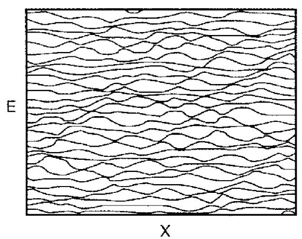
FIG. 16.: The motion of eigenenergies as a function of an external parameter $X$. Many avoided crossings due to level repulsion can be seen, indicating that the level statistics at any fixed value of $X$ is predominantly of Wigner–Dyson type. This picture illustrates results of a calculation for the hydrogen atom in a strong magnetic field by Goldberg et al. [162]. Taken from Ref. [163].

many avoided crossings, see Fig. 16. We consider the parameter $X$ as a function of a fictitious time $t$, $X=X(t)$. Suppose that at time $t=0$, the system is prepared in a high–lying eigenstate of $H(X(0))$. Wilkinson showed that with increasing $t$, the occupation probability of eigenstates of $H(X(t))$ spreads diffusively from the initially prepared state. The parameter $\kappa\propto dX/dt$ measures the non–adiabaticity of the change of $H$. For small $\kappa$, the diffusion process is governed by Landau–Zener transitions at the avoided crossings. The diffusion constant is proportional to $\kappa^{(\beta+2)/2}$ where $\beta$ labels the three symmetry classes. This reflects the power law $s^{\beta}$ of the nearest neighbor spacing distributions for small spacings. It is argued that, for large $\kappa$, the diffusion is governed by Ohmic dissipation and the diffusion constant is proportional to $\kappa^{2}$, independent of the symmetry class. The statistics of the avoided crossings was worked out in Ref. [164]. In recent, related work, Wilkinson and Austin [165] found a diffusion constant proportional to $\kappa^{2}$ for $\beta=1$. This is in agreement with the Kubo formula (see Sec. VI C 1). However, there is a limiting value of $\kappa^{2}$ beyond which the rate is lower. To test these results, these authors also performed numerical studies involving random band matrices. This study suggests that the transition mechanism is different from the above mentioned discussion. Simultaneously, Bulgac, Do Dang and Kusnezov [166] performed closely related studies.

A useful local measure of the parametric dependence of eigenvalues is the curvature

$$K_{n}=\frac{d^{2}E_{n}(X)}{dX^{2}}\Bigg{|}_{X=0}$$ (198)

of the level motion. Indeed, $|K_{n}|$ takes large values at the avoided crossings. Several authors [167, 168, 169] used $K_{n}$ or related quantities to investigate the transition from regular to chaotic motion. Another measure is the distribution $P(K)$ of curvatures. We drop the index $n$ because $P(K)$ must be the same for all eigenvalues. Gaspard et al. [170, 171] investigated $P(K)$ in the fully chaotic regime. These authors used arguments involving the Pechukas gas [172] and the generalized Calogero–Moser system [173, 174] to derive the asymptotic behavior of $P(K)$ for large $K$. They found that this form is universal and given by $1/|K|^{\beta+2}$. As in the case of the diffusion of occupation probabilities discussed above, this form is due to level repulsion since roughly $|K|\propto 1/s$. The universal character of this result was numerically confirmed in Refs. [175, 176, 177, 178] for several different systems. In studying the kicked top, Zakrzewski and Delande [177] conjectured that the full distribution is given by

$$P(k)=\frac{c_{\beta}}{(1+k^{2})^{(\beta+2)/2}}$$ (199)

where the normalization constants read $c_{1}=1/2$, $c_{2}=1/2\pi$ and $c_{4}=8/3\pi$. The dimensionless curvature $k=DK/\pi\beta\langle(dE_{n}/dX)^{2}\rangle$ is given in terms of the mean level spacing $D$ and the mean square level velocity $\langle(dE_{n}/dX)^{2}\rangle$. This quantity is independent of the index $n$. Using the supersymmetry method, von Oppen [179, 180] could prove that the conjecture (199) is indeed true. He used a random matrix model defined through the Hamiltonian

$$H(X)=H_{1}\cos X+H_{2}\sin X$$ (200)

in which both $H_{1}$ and $H_{2}$ belong to the same symmetry class. Several authors have stressed that at this point a caveat is in order: Second order perturbation theory yields an exact expression [179] for the curvature (198) in the model (200). Consequently, formula (199) is universal only for those models which yield an equivalent expression for the curvature. The class of, in this sense, equivalent models, however, is obviously very large. Furthermore, the tail of the distribution is expected to be rather insensitive to the particular model because it is directly related to the spacing distribution. In numerical simulations of billiard systems, Li and Robnik [181] found deviations from the formula (199). Recently, Yurkevich and Kravtsov [182] calculated analytically corrections to this formula.

2 Parametric correlation functions

In contrast to the previous section we consider now two different points $X$ and $X^{\prime}$ in the space of the parameter which governs the level motion. We study the correlation of $E_{n}(X)$ and $E_{m}(X^{\prime})$ as function of the separation in energy and in parameter value. For $X=X^{\prime}$ we have to recover the universal spectral correlations of RMT. New universal features can only be expected on scales on which the gross features of the system play no role, i.e. on the scale of the mean level spacing $D$. We therefore define the unfolded energies $\varepsilon_{n}(X)=E_{n}(X)/D$. We must also unfold the level motion. The appropriate scale is given by the velocity $d\varepsilon_{n}(X)/dX$. We define the new parameter

$$x=\sqrt{\left\langle\left(\frac{d\varepsilon_{n}(X)}{dX}\right)^{2}\right\rangle}\,X\ .$$ (201)

The average is performed either over the spectrum or, in an analytical calculation, over the ensemble. We recall that the same average is used for the normalization of the curvature parameter $k$ below Eq. (199).

Goldberg et al. [162] introduced the parametric number variance as a probe of correlations between different points in parameter space. The cumulative spectral function or staircase function,

$$\widehat{\eta}(\varepsilon,x)=\sum_{n=1}^{N}\Theta(\varepsilon-\varepsilon_{n}(x))$$ (202)

serves to define the parametric level number variance

$$v(x)=\left\langle\Big{(}\widehat{\eta}(\varepsilon,\overline{x}-x/2)-\widehat{\eta}(\varepsilon,\overline{x}+x/2)\Big{)}^{2}\right\rangle$$ (203)

which is obtained by averaging over both the spectrum (or the ensemble) and over the position of the midpoint $\overline{x}$ between two points in parameter space, keeping the distance $x$ fixed. Note that $v(x)$ is not directly related to the spectral level number variance $\Sigma^{2}(L)$: At $x=0$, the function $v(x)$ vanishes by definition. With increasing $x$, the two staircase functions in Eq. (203) get more and more “out of phase”. Hence, we expect that $v(x)$ is a monotonically increasing function of $x$.

Another natural measure of parametric level correlations is the correlation function of the velocity of a fixed eigenvalue $\varepsilon_{n}$ taken at two different points $\overline{x}-x/2$ $\overline{x}+x/2$

$$c(x)=\left\langle\frac{\partial\varepsilon_{n}(\overline{x}-x/2)}{\partial\overline{x}}\frac{\partial\varepsilon_{n}(\overline{x}+x/2)}{\partial\overline{x}}\right\rangle\ .$$ (204)

This function was introduced by Szafer and Altshuler [183] who studied a disordered electronic system in the form of a ring threaded by a magnetic flux. Using diagrammatic perturbation theory, these authors [184] found that beyond a critical regime the correlator (204) becomes independent of any system properties and inversely proportional to the squared flux ($x^{2}$ in the present notation). Together with the investigations by Goldberg et al., this gave the first clear indication that parametric correlations of level motion possess universal features.

Beenakker [185] argued that it ought to be possible to extract such universal features from the standard concepts of Random Matrix Theory. Indeed, Dyson’s Brownian motion [126, 127] and the Pechukas gas [172] both model the motion of levels as function of a fictitious time $t$. Beenakker studied Dyson’s Brownian motion under the crucial assumption that $t$ can be identified with the square of the parameter which governs the level motion. He found that the smooth behavior in $x$ of the correlator (204) is universally given by

$$c_{\beta}(x)\simeq-\frac{2}{\pi^{2}\beta x^{2}}\qquad{\rm for}\qquad x\gg 1\ .$$ (205)

This confirmed the result of Szafer and Altshuler in the unitary case $\beta=2$. The restriction $x\gg 1$ is not imposed by Dyson’s Brownian motion model itself, but is only due to the particular method chosen in Ref. [185] to derive Eq. (205). Beenakker pointed out that the universality of his result confirms the fact that parametric correlations are dominated by level repulsion and thus uniquely determined by the symmetry class. The specific physical realization of the parameter $X$ is immaterial. In the unitary case, the result (205) was also obtained by Brezin and Zee [186] who used a diagrammatic expansion.

Within the supersymmetric $\sigma$ model, Simons and Altshuler [187, 188] simultaneously derived exact expressions for the parametric density–density correlator at two different energies $\overline{\varepsilon}-\varepsilon/2$ and $\overline{\varepsilon}+\varepsilon/2$,

$$k_{\beta}(\varepsilon,x) = \sum_{n,m=1}^{N}\Big{\langle}\delta(\overline{\varepsilon}-\varepsilon/2-\varepsilon_{n}(\overline{x}-x/2))$$ (207)

$$\qquad\qquad\qquad\delta(\overline{\varepsilon}+\varepsilon/2-\varepsilon_{m}(\overline{x}+x/2))\Big{\rangle}-1$$

and the parametric current–current correlator at fixed energy separation

$$\widetilde{c}_{\beta}(\varepsilon,x)=\frac{1}{\sum_{n,m=1}^{N}\left\langle\delta(\varepsilon_{n}(\overline{x}-x/2)-\varepsilon_{m}(\overline{x}+x/2))-\varepsilon)\right\rangle}$$ (208)

$$\quad\sum_{n,m=1}^{N}\bigg{\langle}\delta(\varepsilon_{n}(\overline{x}-x/2)-\varepsilon_{m}(\overline{x}+x/2))-\varepsilon)\frac{\partial\varepsilon_{n}(\overline{x}-x/2)}{\partial\overline{x}}\frac{\partial\varepsilon_{m}(\overline{x}+x/2)}{\partial\overline{x}}\bigg{\rangle}\ .$$ (209)

(210)

The two correlators (207) and (210) are connected through a Ward identity. Hence, we restrict ourselves to the density–density correlator (207). Simons and Altshuler studied a disordered system. They used Efetov’s supersymmetric non–linear $\sigma$ model [44]. They point out that the same results can be derived starting from a random matrix model in the spirit of Ref. [46]. The integral representations in the three universality classes read

$$k_{1}(\varepsilon,x) = {\rm Re}\int_{-1}^{+1}d\lambda\int_{1}^{\infty}d\lambda_{1}\int_{1}^{\infty}d\lambda_{2}\frac{(1-\lambda^{2})(\lambda-\lambda_{1}\lambda_{2})^{2}}{(2\lambda\lambda_{1}\lambda_{2}-\lambda^{2}-\lambda_{1}^{2}-\lambda_{2}^{2}+1)^{2}}$$ (212)

$$\quad\exp\left(-\frac{\pi^{2}x^{2}}{4}(2\lambda_{1}^{2}\lambda_{2}^{2}-\lambda^{2}-\lambda_{1}^{2}-\lambda_{2}^{2}+1)-i\pi\varepsilon^{+}(\lambda-\lambda_{1}\lambda_{2})\right)$$

$$k_{2}(\varepsilon,x) = \frac{1}{2}{\rm Re}\int_{-1}^{+1}d\lambda\int_{1}^{\infty}d\lambda_{1}\exp\left(-\frac{\pi^{2}x^{2}}{2}(\lambda_{1}^{2}-\lambda^{2})-i\pi\varepsilon^{+}(\lambda-\lambda_{1})\right)$$ (213)

$$k_{4}(\varepsilon,x) = \frac{1}{2}{\rm Re}\int_{1}^{\infty}d\lambda\int_{-1}^{+1}d\lambda_{1}\int_{-1}^{+1}d\lambda_{2}\frac{(\lambda^{2}-1)(\lambda-\lambda_{1}\lambda_{2})^{2}}{(2\lambda\lambda_{1}\lambda_{2}-\lambda^{2}-\lambda_{1}^{2}-\lambda_{2}^{2}+1)^{2}}$$ (215)

$$\quad\exp\left(-2\pi^{2}x^{2}(\lambda_{1}^{2}+\lambda_{2}^{2}+\lambda^{2}-2\lambda_{1}^{2}\lambda_{2}^{2}-1)+i2\pi\varepsilon^{+}(\lambda-\lambda_{1}\lambda_{2})\right)$$

where the energy difference $\varepsilon$ is given an imaginary increment. The symplectic case was worked out in Ref. [189]. For $x=0$, Efetov’s integral representations of the spectral two–point functions [44] are recovered. For $\beta=2$, Beenakker and Rejai [163] performed a calculation in the framework of Dyson’s Brownian motion model which yields full agreement with the results of Simons and Altshuler. From the definition (210) it is obvious that for large $x$, the current–current correlator $\widetilde{c}(0,x)$ at zero energy separation has to approximate the velocity correlator $c(x)$ defined in Eq. (204). Using the Ward identity mentioned above, the result (205) can indeed be rederived. Remarkably, no integral representation of the form (215) valid for arbitrary $x$ could

FIG. 17.: The parametric velocity correlators $c_{\beta}(x)$, obtained from numerical simulations. The solid line is the GOE result ($\beta=1$), the dashed line is the GUE result ($\beta=2$). The curves have a very small numerical error. Taken from Ref. [190].

be derived for $c(x)$ yet. Mucciolo [190, 191] obtained $c_{\beta}(x)$ by extensive numerical simulations for orthogonal ($\beta=1$) and unitary ($\beta=2$) symmetry. He used random matrices of the form (200). The results are shown in Fig. 17.

Just as its spectral analogue, the parametric level number variance can be expressed in terms of the two–point function,

$$v_{\beta}(x)=2\lim_{x^{\prime}\to 0}\int_{-\infty}^{0}d\varepsilon\int_{-\infty}^{\varepsilon}d\varepsilon^{\prime}\left(k_{\beta}(\varepsilon^{\prime},x^{\prime})-k_{\beta}(\varepsilon^{\prime},x)\right)\ .$$ (216)

For small values of $x$, these integrals can be worked out. For the unitary and the orthogonal case, one finds

$$v_{\beta}(x)\simeq\sqrt{\frac{2}{\pi}}|x|\qquad{\rm for}\qquad x\to 0\ .$$ (217)

For larger values of $x$, the parametric level number variance can be obtained by numerical integration of Eq. (216). It turns out that $v_{1}(x)$ and $v_{2}(x)$ begin to differ. A discrepancy with the semiclassical formula in Ref. [162] was attributed by Simons and Altshuler to the failure of the semiclassical method for small $x$.

The results derived within the supersymmetric non–linear $\sigma$ model give the most general proof of the universality of parametric correlations. Although experiments and numerical simulations have verified this universality, see Ref. [192], deviations have also been found.

Naturally, the question arises whether observables involving the wave functions also possess universal features. Using the Gaussian processes discussed in the following section, Attias and Alhassid [193] studied the normalized energy–dependent parametric overlap of wave functions $\psi_{n}(\vec{r},x)$ at different values of the dimensionless parameter $x$,

$$\widetilde{o}_{\beta}(\varepsilon,x) = \frac{1}{\sum_{n,m=1}^{N}\left\langle\delta(\varepsilon_{n}(\overline{x}-x/2)-\varepsilon_{m}(\overline{x}+x/2))-\varepsilon)\right\rangle}$$ (220)

$$\qquad\sum_{n,m=1}^{N}\Big{\langle}|\langle\psi_{n}(\vec{r},\overline{x}-x/2)|\psi_{m}(\vec{r},\overline{x}+x/2)\rangle|^{2}$$

$$\qquad\qquad\qquad\qquad\delta(\varepsilon_{n}(\overline{x}-x/2)-\varepsilon_{m}(\overline{x}+x/2))-\varepsilon)\Big{\rangle}\ .$$

With the supersymmetry method, exact expressions were given for $\beta=1$ and $\beta=2$ and compared to numerical simulations of the Anderson model. In the orthogonal case and for zero energy separation, the overlap is Lorentzian. As $\varepsilon$ increases, the shape changes, and the peak moves from $x=0$ to larger values of $x$.

Mucciolo et al. [194] also studied the dependence of wave functions in the chaotic regime on a parameter, using the full joint distribution function

$$w_{\beta}(\overline{a},a,X) = \Big{\langle}\delta(\overline{a}-a/2-V|\psi_{n}(\vec{r},\overline{x}-x/2)|^{2})$$ (222)

$$\qquad\qquad\delta(\overline{a}+a/2-V|\psi_{n}(\vec{r},\overline{x}+x/2)|^{2})\Big{\rangle}\ .$$

They showed that in the limit of small $x$, this distribution has asymptotically the universal form

$$w_{\beta}(\overline{a},a,X)\simeq P_{\beta}(\overline{a})\frac{1}{2\pi x\sqrt{\overline{a}}}B_{\beta}\left(\frac{a}{2\pi x\sqrt{\overline{a}}}\right)\qquad{\rm for}\qquad x\to 0$$ (223)

where $P_{\beta}$ is the $\chi^{2}$ distribution defined in Eq. (147). The function $B_{\beta}$ is also universal and depends only on the symmetries of the system. In the unitary case, the function $B_{2}$ was given explicitly.

3 Gaussian random processes

The universality of the parametric correlation functions suggests the existence of a proper generalization of the Gaussian ensembles. This generalization should lead naturally to the parametric correlations. In the context of parametric level motion, and for numerical simulations of the diffusion constants discussed in Sec. III H 1, Wilkinson [161] introduced a parameter dependence in the GOE. Let the Gaussian distributed white–noise matrices $W_{nm}(X)$ have zero mean values and a second moment given by

$$\overline{W_{nm}(X)W_{n^{\prime}m^{\prime}}(X^{\prime})}=(\delta_{nn^{\prime}}\delta_{mm^{\prime}}+\delta_{mn^{\prime}}\delta_{nm^{\prime}})\delta(X-X^{\prime})\ .$$ (224)

A parametric dependence of the random Hamiltonian $H$ can then be defined by convoluting these white noise functions with a smoothly varying function $h(X)$,

$$H_{nm}(X)=\int_{-\infty}^{+\infty}W_{nm}(X^{\prime})h(X-X^{\prime})dX^{\prime}\ .$$ (225)

For the second moments of the matrix elements this yields

$$\overline{H_{nm}(X)H_{n^{\prime}m^{\prime}}(X^{\prime})} = (\delta_{nn^{\prime}}\delta_{mm^{\prime}}+\delta_{mn^{\prime}}\delta_{nm^{\prime}})\widehat{f}(X-X^{\prime})$$ (226)

$$\widehat{f}(X) = \int_{-\infty}^{+\infty}h(X-X^{\prime})h(-X^{\prime})dX^{\prime}\ .$$ (227)

The function $\widehat{f}(X)$ is translation invariant by construction but not necessarily symmetric in $X$. In studying related questions in a different context, Ko et al. [195] and Brink et al. [196] had earlier introduced distributions defined by an equation similar to Eq. (227). In these cases, however, the function $f(X)$ had an additional dependence on the matrix indices, leading to a band structure of the matrices. More recently, related studies have been performed by Bulgac et al. [166]. From the point of view of statistical mechanics, the introduction of the dependence on such a parameter $X$ in Eqs. (224) and (227) is tantamount to the introduction of another dimension: The zero–dimensional Random Matrix Theory becomes one–dimensional. In Sec. VII A 1, we discuss a related important process, the free propagation of a time–dependent random matrix.

A suitable unifying generalization of Wilkinson’s ideas was introduced by Alhassid and Attias [193, 197] in the form of the Gaussian random process. Let $H(X)$ denote matrices of dimension $N$, with volume element $d[H(X)]$, which depend on the parameter $X$. For all $X$, the matrices belong to the same symmetry class labeled by $\beta$. The Gaussian Orthogonal, Unitary and Symplectic Processes, GOP, GUP and GSP, respectively, are defined through the probability density

$$P(H(X))\propto\exp\left(-\frac{\beta}{2v^{2}}\int dX\int dX^{\prime}{\rm tr}H(X)K(X,X^{\prime})H(X^{\prime})\right)$$ (228)

where $K(X,X^{\prime})$ is a scalar function. Since the distribution is Gaussian, it is completely determined by the first two moments

$$\overline{H_{nm}(X)} = 0$$ (229)

$$\overline{H_{nm}(X)H_{n^{\prime}m^{\prime}}(X^{\prime})} = \frac{v^{2}}{2\beta}f(X,X^{\prime})g_{\beta,nmn^{\prime}m^{\prime}}$$ (230)

where $g_{1,nmn^{\prime}m^{\prime}}=(\delta_{nn^{\prime}}\delta_{mm^{\prime}}+\delta_{mn^{\prime}}\delta_{nm^{\prime}})$ in the orthogonal and $g_{2,nmn^{\prime}m^{\prime}}=2\delta_{nm^{\prime}}\delta_{n^{\prime}m}$ in the unitary case. Equation (230) bears a close formal relationship to Eq. (227). It is assumed, however, that $f$ be both translation invariant and symmetric, $f(X,X^{\prime})=f(|X-X^{\prime}|)$, and that $f(0)=1$. This implies that $K(X,X^{\prime})$ also obeys $K(X,X^{\prime})=K(|X-X^{\prime}|)$. The kernel $K$ and the function $f$ are related via their Fourier transforms $\widetilde{K}(k)$ and $\widetilde{f}(k)$ by

$$\widetilde{K}(k)=1/\widetilde{f}(k)\ .$$ (231)

All Gaussian processes can be constructed from the elementary Gaussian process defined by the white noise weight functions

$$f(X-X^{\prime})=\delta(X-X^{\prime})\qquad{\rm and}\qquad K(X-X^{\prime})=\delta(X-X^{\prime})\ .$$ (232)

The elementary Gaussian process formally includes also the case of a Gaussian white noise potential. To see this, we interpret the parameter $X$ as the $d$–dimensional position vector and insert the Fourier transform of Eq. (231) into Eq. (228) for matrix dimension $N=1$.

As an illustration, we present one of the examples given in Refs. [197, 193]. We consider the Ornstein–Uhlenbeck Gaussian process [198]

$$f(X) = \exp(-\gamma|X|)\qquad{\rm and}$$ (233)

$$K(X-X^{\prime}) = \frac{1}{2\gamma}\left(\gamma^{2}-\frac{\partial^{2}}{\partial X^{2}}\right)\delta(X-X^{\prime})$$ (234)

where $\gamma$ is a positive constant. If the parameter $X$ is identified with time $t$, the weight functions (234) lead to the action of a freely propagating matrix with quadratic potential, see Eq. (7). Naturally, both the physical and mathematical significance of $X$ can be very different for different choices of weight functions. In Refs. [193, 197], the relationship between the Ornstein–Uhlenbeck process and Dyson’s Brownian motion model is also discussed from the viewpoint of Gaussian processes.

IV Many–body systems

We deal with self–bound systems consisting of several or many particles which interact through two–body forces. In the case of atomic nuclei, the particles are nucleons and in the case of atoms and molecules, they are ions and electrons. We can cover only a small fraction of the enormous wealth of published material. Atomic nuclei display considerable complexity and have been studied extensively. This is why we put emphasis on this field which is discussed in Sec. IV A, while atoms and molecules are the subject of Sec. IV B. Some general questions arising in the context of many–body systems are addressed in Sec. IV C.

A Atomic nuclei

Medium–weight or heavy nuclei are complex many–body systems par excellence [63, 199]. A nucleus with mass number $A=N+Z$ contains $N$ neutrons and $Z$ protons. The size of a nucleon and the average distance between the nucleons are both about 1 fm. The range of the strong interaction is also of the order of 1 fm. The energy scale is MeV (Mega electron volts).

As outlined in the Historical Survey, the high complexity of nuclei prompted the introduction of statistical concepts already in the early days of nuclear physics. This eventually led to Random Matrix Theory. This development has had enormous impact on statistical many–body physics at large. To prepare the ground for the introduction of statistical concepts, we present in Sec. IV A 1 a very brief introduction into the most essential aspects of nuclear physics. In Secs. IV A 2 and IV A 3, we collect, respectively, the evidence for random matrix properties of spectral fluctuations, and data on the distribution of scattering parameters and widths. All theoretical models for the nucleus are effective, i.e., do not start from the basic nucleon–nucleon interaction. Thus, it is important to see whether the fluctuation properties displayed by the data are also borne out in model calculations. This is discussed in Sec. IV A 4. In Sec. IV A 5 we summarize some of the work which employs Random Matrix Theory as a tool to obtain upper bounds or values for the strengths of invariance– and/or symmetry–breaking forces.

The are numerous reviews on Random Matrix Theory in nuclear physics. We mention Refs. [9, 200, 25, 201, 18, 202, 203, 204, 205].

1 Basic features of nuclei

The cross section for the elastic scattering of slow neutrons on heavy nuclei displays sharp resonances with widths ranging from about 3 meV to 1 eV, and with spacings of about 10 eV, see Fig. 2. These resonances cannot be due to a single interaction between the incident neutron and a target nucleon. Indeed, a straightforward estimate shows that the inverse reaction time for such a two–body collision yields a value for the resonance width which is in the MeV range. The small observed widths correspond to much longer interaction times. This requires that many nucleons in the target participate in the reaction, and that each resonance has a complex wave function. While it may thus be difficult to account for the properties of individual resonances, the average of the cross section over many resonances can be obtained by the following statistical argument. The available energy is assumed to be spread uniformly over all participating nucleons in such a way that the target nucleus and the incident neutron together form a new system, the compound nucleus. This system equilibrates and loses memory of its mode of formation before it decays. As a consequence, formation and decay of the compound nucleus are independent processes. This is the essence of Bohr’s picture [10] of the compound nucleus.

The picture yields a formula for the average cross section $\langle\sigma_{ab}\rangle$. The incident channel (in our example, the slow neutron) is denoted by $a$. The average probability for formation of the compound nucleus from the incident channel is given by the transmission coefficient $T_{a}$. The decay of the compound nucleus into other channels $c$ is likewise governed by associated transmission coefficients $T_{c}$. Depending on the available energy, $c$ may stand for an inelastically scattered neutron, a proton, an $\alpha$ particle, etc. In Bohr’s statistical picture, $\langle\sigma_{ab}\rangle$ is proportional to $T_{a}G_{b}$ where $G_{b}$ is the probability for the decay into channel $b$. Since the nucleus has to decay into one of the $\Lambda$ open channels, we have $\sum_{b=1}^{\Lambda}G_{b}=1$. On the other hand, $G_{b}$ must be proportional to $T_{b}$. Thus, $G_{b}=T_{b}/\sum_{c=1}^{\Lambda}T_{c}$. This yields the Hauser–Feshbach formula [103],

$$\langle\sigma_{ab}\rangle=C_{\rm kin}\frac{T_{a}T_{b}}{\sum_{c=1}^{\Lambda}T_{c}}\ .$$ (1)

Kinematic factors have been absorbed in the constant $C_{\rm kin}$.

These stochastic concepts received strong support when in 1966 Ericson [24] showed that the nuclear cross section can be viewed as a random variable. His ideas apply in the regime where the average resonance width is much larger than the mean level spacing, i.e. in the regime of strongly overlapping resonances. At any one energy, the cross section is due to the superposition of many resonances. If each resonance contributes a random amplitude, the cross section fluctuates randomly versus energy. Minima and maxima are not related to individual resonances. Nevertheless, the cross section is fully reproducible. Therefore, the fluctuations do not represent white noise, but internal stochastic behavior of the compound system.

Prior to Ericson’s observation, the discovery of shell structure in nuclear binding energies had led to quite different a picture of the nucleus. At certain values of the neutron and proton numbers $N$ and $Z$, the nuclear binding energy displays maxima. As in atomic physics, these maxima can be explained in the framework of a shell model [206]. In contrast to the atomic case, a strong spin–orbit force has to be invoked to describe the data. In the nuclear shell model, each nucleon moves independently in a mean field $U$ generated by all other nucleons. The Hamiltonian takes the form

$$H = \sum_{k=1}^{A}\left(T(k)+U(k)\right)+H_{\rm res}$$ (2)

$$H_{\rm res} = \sum_{k<l}W(k,l)-\sum_{k=1}^{A}U(k)\ .$$ (3)

Here, $T(k)$ is the kinetic energy and $W(k,l)$ is the two–body interaction between nucleons $k$ and $l$. The difference $H_{\rm res}$ between the true two–body interaction and the mean field is referred to as the residual interaction. (This picture is oversimplified and does not account for the strong repulsion between pairs of nucleons.) The model is very successful in accounting for the low–energy spectra of many nuclei, particularly when the residual interaction is chosen phenomenologically. In the space of Slater determinants of shell–model states, the Hamilton matrix acquires a highly complex structure, making it a well–suited object for a statistical approach. In this basis, the matrix elements of $H_{\rm res}$ have a nearly Gaussian distribution. This fact links the shell model to the random matrix approach to nuclear reactions.

Nuclei are capable of yet another type of motion. This was discovered shortly after the emergence of the shell model. A nucleus can be viewed as a piece of dense but elastic matter with spherical or ellipsoidal shape. This object can vibrate and, in the case of deformation, rotate. Collective modes, the quantal manifestations of such motion, occur in many nuclei. The minimum rotational energy $E(I)$ a nucleus must have for a given total spin $I$ defines a lower bound for its total energy $E$. In the $(E,I)$ plane, the curve of $E(I)$ versus $I$ has parabolic shape. It is called the yrast line. This curve defines rotation without inner excitation (“cold rotation”). Excitations heat up the system. On the yrast line, the collective motion decays through the emission of electric quadrupole ($E2$) radiation. A state of spin $I$ on the yrast line decays into a state of spin $I-2$, and so on. States connected by a sequence of such strong $E2$ transitions form a rotational band. Near the yrast line, the members of a rotational band are characterized by the $K$ quantum number. This is the projection of the intrinsic angular momentum (caused by single–particle excitations) onto the symmetry axis of the deformed nucleus. Collective excitations often follow an easily predictable pattern, leaving little room for the kind of stochastic behavior modeled by random matrices.

Collective excitations at low energy and low angular momentum values are often modeled in terms of the Interacting Boson Model (IBM) [207]. Due to the strong pairing force in the nuclear Hamiltonian, pairs of protons or of neutrons couple to bosonic pairs which form the basic ingredients of the model. In its basic version, the model contains Bosons with spin zero ($s$ Bosons) and Bosons with spin two ($d$ Bosons). For nuclei with even $A$, the IBM Hamiltonian is solely expressed in terms of these Bosons. Nucleons do not appear. The Hamiltonian has the form

$$H=c_{0}n_{d}+c_{2}Q^{\chi}\cdot Q^{\chi}+c_{1}\vec{L}^{2}\ .$$ (4)

Here $\vec{L}$ is the total angular momentum operator and $c_{0}$, $c_{1}$ and $c_{2}$ are parameters. The operator $n_{d}$ counts the number of $d$ Bosons. The quadrupole operator $Q^{\chi}$ models the deformation of the nucleus. It depends on a parameter $\chi$. The Hamiltonian (4) possesses a U(6) and an O(3) symmetry, corresponding to the conservation of Boson number and angular momentum. Three different group chains connect U(6) with O(3). Each chain represents a dynamical symmetry which is realized in the Hamiltonian (4) for a certain choice of parameters. Physically, these dynamical symmetries correspond to vibrational, rotational and deformation–instable nuclei. Every IBM Hamiltonian describing a real nucleus corresponds to a point in the space of parameters of the IBM. The IBM can be viewed as a mapping of the space of shell–model Slater determinants onto a — drastically smaller — sub–space spanned by bosonic wave functions.

In summary, independent–particle motion with coupling through the residual interaction, collective modes due to deformation, and a stochastic approach form the main ingredients of nuclear theory. These elements have different relative weights at different excitation energies and mass numbers $A$.

For the statistical analysis, the concept of the spreading width has proven very useful. We consider a nucleus modeled by a Hamiltonian $H=H_{0}+V$. The first part, $H_{0}$, describes the sub–system which is pure with respect to symmetries, invariances or other properties. The second part, $V$, is a perturbation which destroys this property. For example, $H_{0}$ conserves time–reversal invariance and $V$ breaks it, or, $H_{0}$ models purely collective motion while $V$ contains single–particle excitations. The influence of the perturbation can most conveniently be measured if the eigenbasis of $H_{0}$ is taken as the “reference frame”. As $V$ increases, an eigenstate of $H$ spreads out, starting from an initial eigenstate of $H_{0}$. The averaged energy scale of this spreading in the spectrum can be shown to be given by the spreading width

$$\Gamma=2\pi\frac{\langle V^{2}\rangle}{D_{0}}$$ (5)

where $D_{0}$ is the mean level spacing due to $H_{0}$ and $\langle V^{2}\rangle$ is the mean square perturbation matrix element. The spreading width $\Gamma$ should not be confused with the decay width of an open quantum system. It is conceptually closely related to the Thouless energy which is used in condensed matter physics, see Sec. VI. The spreading width is frequently used to characterize the strength of a perturbation $V$. This is done because $\Gamma$, in contrast to both the matrix elements of $V$ and $H_{0}$, depends only very little on excitation energy or mass number. Indeed, $D_{0}$ decreases essentially exponentially with excitation energy $E$, and the same is true for $\langle V^{2}\rangle$ because the complexity of eigenstates of $H_{0}$ grows strongly with $E$. It can be shown [18] that these exponential dependences cancel in the ratio $\Gamma$ of Eq. (5).

2 Spectral fluctuations

Data of sufficiently high quality to test spectral fluctuations in nuclei are available only in restricted energy windows. It is crucial that sequences of levels of the same spin and parity be complete (no missing levels) and pure (no levels with wrong quantum numbers). Spectra which contain levels of all spins and parities yield a Poisson distribution [208, 209], see Sec. III B 5. One such window is defined by the scattering of slow neutrons [2, 210, 211, 212], see Fig. 2, and of protons at the Coulomb barrier [213]. Earlier than in other areas of physics, the energy resolution and the size of the data set attained here were sufficient for a statistical analysis. In 1982, Haq, Pandey and Bohigas [26] analyzed the set of 1726 nuclear spacings then available from such data. This “nuclear data ensemble” is a combination of data on neutron [214, 215] and proton [216] resonances. For neutrons, about 150 to 170 $s$ wave resonances per nucleus located typically about 9 MeV above the ground state, contribute to the ensemble. For protons, the sequences consist of 60 to 80 levels per nucleus. After separate unfolding, the sequences were lumped together and analyzed. Remarkable agreement of both spacing distribution (see Fig. 1) and spectral rigidity with GOE predictions was found. Three– and four–level correlations also agree well [217]. Recently, Lombardi, Bohigas and Seligman [84] analyzed the spectral two–level form factor of the nuclear data ensemble and applied the GSE test discussed in Sec. III B 6. Again, consistence with random matrix predictions was found.

Another window for a test of spectral fluctuations exists in the ground–state domain. This region was first investigated by Brody et al. [218] who found some evidence for GOE–like behavior. A much more detailed study is due to von Egidy, Behkami and Schmidt [219, 220]. The data set of this analysis consists of 1761 levels from 75 nuclides between ²⁰F and ²⁵⁰Cf. The set is obtained from the analysis of $(n,\gamma)$ reactions. The data are separated into pure sequences. The combined nearest neighbor spacing distribution lies between a Poisson distribution and the Wigner surmise. Abul–Magd and Weidenmüller [221] divided the data set of Ref. [219] into a number of groups and analyzed the spacing distribution and the spectral rigidity within each group. It was found that the collective states with spin $J$ and parity $\pi$ values of $J^{\pi}=2^{+}$ and $4^{+}$ in rotational nuclei show Poisson characteristics whereas the fluctuations of the remaining levels are much closer to GOE predictions. A more complete study along similar lines is due to Shriner, Mitchell and von Egidy [222]. These authors analyzed a data set of 988 spacings from 60 nuclides for which the level schemes are believed to be complete in an energy interval starting with the ground state, and over some range of angular momentum values. The results show a strong mass dependence. The spacing distributions of the lighter nuclides are close to GOE while those of the heavier ones are closer to a Poisson distribution, see Fig. 18.

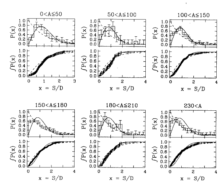
FIG. 18.: Nearest neighbor spacing distributions and cumulative spacing distributions for all levels in six different regions of the nuclear mass parameter $A$. The dashed lines show the behavior for the Poisson distribution, and the smooth solid lines show it for the Wigner surmise. Taken from Ref. [222].

This suggests that the coupling of independent particles by the residual interaction generically leads to GOE behavior, and that collectivity is the origin of Poisson statistics. Further support for this hypothesis comes from the investigation of spin and shape effects in Ref. [222], although the number of states available was rather small. The spacing distributions of the $2^{+}$ and $4^{+}$ states in heavier and deformed nuclides (where collectivity is strongest) are close to Poisson while those of the $0^{+}$ and $3^{+}$ states in the same nuclides and the $2^{+}$ and $4^{+}$ states in spherical nuclides are close to GOE. A Poisson distribution would be expected for a superposition of states with different quantum numbers [23], see Sec. III B 5. Candidates for such unidentified conserved quantum numbers are isospin $T$ and the $K$ quantum number introduced in the previous section. However, even a weak breaking of the symmetry associated with $T$ or $K$ quickly leads to GOE statistics, see Sec. III F 3. In the data of Shriner et al. there is a hint towards an interuption of the gradual transition from Wigner–Dyson to Poisson statistics in the mass region $180<A\leq 210$. Abul–Magd and Simbel [223] argued that this could be related to the occurence of oblate deformation in this mass region.

Another window exists in deformed rare–earth nuclei with mass numbers $A$ between 155 and 185. In contrast to the cases discussed above, the data are taken near the yrast line and contain much higher spin values. Garrett and co–workers [224, 225] analyzed 2522 level spacings. Very recently, the analysis was extended [226] and includes now 3130 spacings. The average spacing was calculated for the total ensemble, before dividing it into pure sequences of fixed spin and parity, because the properties of the deformed nuclei in this mass region are known to be similar. The authors state that, for this and other reasons, the usual method to determine the average spacing for individual pure sequences can be replaced by this procedure of combining the sequences in the yrast region. The resulting spacing distribution is the closest to a Poisson distribution yet obtained except for a statistically significant suppression of very small spacings. It is argued that this suppression indicates that $K$ is (nearly) a good quantum number for the low–lying states in deformed rare–earth nuclei.

Little is known about the spectral fluctuations of individual nuclei. The most complete data sets available are probably the ones for ²⁶Al, analyzed by Mitchell et al. [227, 228], and for ¹¹⁶Sn, analyzed by Raman et al. [229]. The results for ²⁶Al are important for the study of symmetry breaking and are discussed in Sec. IV A 5. The authors of Ref. [229] present an almost complete level scheme of ¹¹⁶Sn from the ground state to a maximum excitation energy of $4.3~{}{\rm MeV}$. The resulting spacing distribution lies between a Poisson and a Wigner distribution. Bybee et al. [230] applied the correlation–hole method (see Sec. III B 4) to spectra of ⁵⁷Co and ¹⁶⁷Er. However, these authors conclude, that the limited sample size of their data yields ambiguous results whereas the spacing distribution and the spectral rigidity are statistically more significant.

In Refs. [225, 226] it is attempted to draw a coherent picture of the results summarized above. In the work of Refs. [224, 225], the value of the mean level spacing, $D=297~{}{\rm keV}$, considerably exceeds the typical size of the interaction matrix elements, $V_{\rm int}<35~{}{\rm keV}$, between the states. Thus, the fluctuations are expected to be close to Poisson. For small spacings $s<70~{}{\rm keV}/D$, a deviation from the Poisson distribution is seen because here $s$ is comparable with $V_{\rm int}/D$. The other extreme is provided by the nuclear data ensemble analyzed in Refs. [26, 217, 84]. Here, the mean level spacing $D$ is much smaller than a typical interaction matrix element, $D\ll V_{\rm int}$. The states are strongly mixed and the fluctuations are GOE. In the case of ¹¹⁶Sn, the mean level spacing $D=110~{}{\rm keV}$ is comparable with the interaction matrix element $V_{\rm int}$, causing the spacing distribution to lie between the Poisson and the Wigner distribution. Figure 19 shows the three windows in which the aforementioned data were taken. This

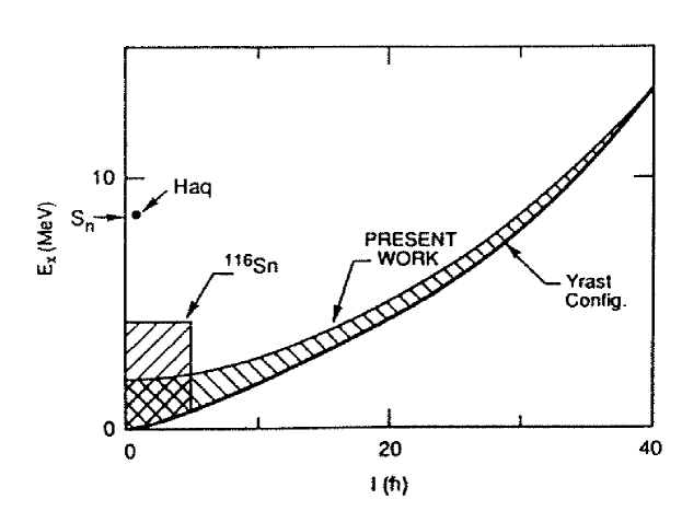
FIG. 19.: The range of excitation energies $E_{x}$ and angular momenta $I$ associated with the three data sets mentioned in the text. The point in this diagram from which the levels for the nuclear data ensemble are taken is labeled with “Haq”. The shaded area labeled “¹¹⁶Sn” indicates the area in the plane from which the data for the analysis of Raman et al. [229] were gathered. The shaded area designated “present work” refers to the analysis of Garrett et al. [224, 225, 226]. The yrast line is shown as a solid line. Taken from Ref. [226].

interpretation suggests a statistical model of the type $H^{(0)}+\alpha H^{(1)}$ where $H^{(0)}$ and $H^{(1)}$ model Poisson and GOE fluctuations, respectively, see Sec. III F. The parameter $\lambda=\alpha/D$ is of the order of $V_{\rm int}/D$.

3 Resonances and scattering

Aside from the resonance positions, data for resonance reactions also yield partial and total widths. RMT predicts the distribution of partial widths to be of Porter–Thomas form, see Sec. III E 1. Prior to a comparison of data with this prediction, it is necessary to remove the penetration factors due to the Coulomb and/or angular momentum barriers from the measured partial widths. Early experimental evidence for the validity of the Porter–Thomas distribution for the resulting “reduced” widths is summarized in Refs. [9] and [200]. Later, the distributions of reduced widths for neutron [215] and proton [231] resonance data were shown to be consistent with the Porter–Thomas law. However, Harney [232] pointed out that a statistically significant test requires many more data than were available at the time. Therefore, Shriner, Mitchell and Bilpuch [233, 234] used another statistical observable. The Porter–Thomas distribution for the reduced widths results from the Gaussian distribution for the reduced width amplitudes, see Sec. III E 1, and that latter distribution is tested. With $n$ the running index of a set of resonances, the reduced width amplitudes $\gamma_{na}$ and $\gamma_{nb}$ for two different channels $a$ and $b$ are taken as two data sets. If two sets $\{x_{1},\ldots,x_{N}\}$ and $\{y_{1},\ldots,y_{N}\}$ have a Gaussian distribution, the linear correlation coefficient

$$\rho(x,y)=\frac{\sum_{n=1}^{N}\left(x_{n}-\langle x\rangle\right)\left(y_{n}-\langle y\rangle\right)}{\sqrt{\sum_{n=1}^{N}\left(x_{n}-\langle x\rangle\right)^{2}\sum_{n=1}^{N}\left(y_{n}-\langle y\rangle\right)^{2}}}$$ (6)

has the property $\rho(x^{2},y^{2})=\rho^{2}(x,y)$. This test is far more sensitive than a comparison with the Porter–Thomas law because it involves the joint moments of the partial width amplitudes $\gamma_{na}$ and $\gamma_{nb}$ and, thus, the relative signs of the amplitudes. This information was provided by the analysis of interference phenomena in the exit channels in proton–induced reactions. The analysis yields a statistically significant confirmation of GOE predictions.

The successful analysis of the distribution of the positions and widths of well–resolved isolated resonances in terms of the GOE implies that compound nucleus scattering itself is a stochastic process and can be modeled by the stochastic scattering problem introduced in Sec. III D. It is assumed that this modeling applies not only in the domain of isolated resonances but also at higher energies where resonances overlap. Apart from kinematic factors, the compound nucleus cross section is then given by the square modulus of the scattering matrix in Eq. (130) of Sec. III D, and the fluctuation properties of compound nucleus cross sections can be predicted. The history of this problem is mirrored in the reviews in Refs. [200, 25, 18]. For a long time, only perturbative solutions were available, valid either for small or for large values of the ratio $\Gamma/D$. Here, $\Gamma$ is the average total width of and $D$ the mean spacing between resonances. Use of the supersymmetry method [46] made it possible to work out the fluctuations of the scattering matrix in all regimes, from isolated resonances to the Ericson regime of strongly overlapping resonances, see Sec. III D 2. The result is also of practical use. An example is the application to reactor physics at low energies, see Ref. [235]. The leading term of an expansion of the result in inverse powers of $\sum_{c=1}^{\Lambda}T_{c}$ yields the Hauser–Feshbach formula (1). Nishioka and Weidenmüller [236] showed that direct reactions can easily be included in the formalism.

The use of the GOE in this model for compound nucleus scattering implies that the internal equilibration time of the nucleus is small in comparison with the decay time $\hbar/\Gamma$. This is true at low incident energies. However, in reactions induced by light ions, $\hbar/\Gamma$ decreases strongly with energy and becomes comparable to the equilibration time for incident energies higher than 10 MeV or so. Then, the compound nucleus can decay before it is completely equilibrated, and the model of Sec. III D 2 must be extended to account for this fact. This is done by using the nuclear shell model and dividing the compound system into classes of states. Each class comprises states with fixed particle–hole number and is represented by a random matrix. Owing to the two–body character of the residual interaction, only neighboring classes are coupled. This coupling is also modeled by random matrices. The total Hamiltonian is then a band matrix whose entries are random matrices. Following earlier work by Agassi, Weidenmüller and Mantzouranis [237] and Feshbach, Kerman and Koonin [238], Nishioka et al. [239] succeeded in calculating the average cross section for this model. They used the supersymmetry method and a loop expansion [240]. The strong breaking of rotation invariance in Hilbert space of this random matrix model amounts to the introduction of a dimension. This is why this model later became important for mesoscopic systems, see Sec. VI C 3. The ideas used in the model have been tested perhaps most stringently in nuclear reactions with isospin mixing, see Sec. IV A 5.

Another approach to compound nucleus scattering considers the scattering matrix itself as the basic random entity and uses the maximum entropy approach to determine the fluctuation properties, see Sec. III D 2. The random transfer matrix technique used in mesoscopic physics (see Sec. VI C 2) can be viewed as an extension of this approach.

4 Model systems

As mentioned above, it is important to test whether spectral fluctuation properties predicted by various nuclear models correctly reproduce the properties of nuclei reviewed in the last two sections. This is true, in particular, because all models of the nuclear many–body problem are effective models based on mean–field approaches.

There are numerous studies of spectral fluctuation properties within the nuclear shell model. Early work is reviewed in Ref. [18]. We only mention the studies of Soyeur and Zuker [241] and of Wong [242] which date back to the early seventies. The former authors found good agreement of the spin $J=2$ states in ²⁴Mg with the Wigner surmise. Wong calculated spectra including several $J$ values whose spacing distributions follow the Poisson law. We can also mention only a few of the recent results. Ormand and Broglia [243] performed realistic shell–model calculations for light nuclei in the mass region $20<A<35$ and for ⁴⁶V. Very good agreement of the spacing distribution and the spectral rigidity with the GOE prediction was found in the region near the ground state. However, in these calculations isospin conservation was assumed, see Sec. IV A 5.

The influence of the mean field was investigated by Drożdż et al. [244] in the spectrum of two–particle two–hole states. As expected on general grounds, there is no level repulsion within a pure mean–field approach. GOE type fluctuations occur when the residual interaction is switched on. Level repulsion arises from particle–hole re–scattering effects. Zelevinsky et al. [205, 245] calculated spectra of light nuclei as a function of the strength of the residual interaction. A relatively weak interaction suffices to produce a Wigner type spacing distribution. This is agreement with the RMT expectations, see Sec. III F.

The distribution of the amplitudes of shell–model wave functions in a fixed basis has also been compared to the GOE prediction [18]. In the ground–state domain, Whitehead et al. [246] and Verbaarschot and Brussaard [247] found deviations from the Gaussian behavior predicted by the GOE. The single–particle states within a major shell are not completely degenerate. The splitting of the single–particle energies counteracts the mixing of states by the residual interaction. Interestingly, Whitehead et al. [246] set up a random matrix with a block structure in the spirit of the Rosenzweig–Porter model to be discussed in Sec. IV B 1. Brown and Bertsch [248] showed that the distribution of the amplitudes becomes Gaussian at higher excitations where the level density is larger. It was also argued by Zelevinsky et al. [249] that calculations with degenerate single–particle energies yield GOE features at lower energies than models which are believed to describe the nucleus in a more realistic fashion. A discussion can be found in Zelevinsky’s review [205]. The decay in time of the compound nucleus has also been the object of several studies. For many (few) open channels, RMT predicts exponential (algebraic) decay [99, 250, 251], respectively. This was compared with model calculations in various regimes [252, 253].

The interplay between collective motion and single–particle effects can ideally be studied in hot rotating nuclei, cf. Sec. IV A 1. The results reviewed in Sec. IV A 2 suggest that collective motion is likely to yield Poisson or harmonic oscillator statistics whereas single–particle effects should lead to GOE behavior. Reviews were given by Åberg [254] and Døssing et al. [255]. Rotational bands exist not only near the yrast line (see Sec. IV A 1), but also at excitation energies of a few MeV above it. At these energies, the rotational bands are mixed by the residual interaction. Thus, a state with spin $I$ does not decay into a single state of spin $I-2$ within the same band, but into several or even many states with spin $I-2$. This phenomenon is referred to as rotational damping and is characterized by a spreading width, see Sec. IV A 1. Experimental and theoretical evidence for rotational damping was given by Leander [256] as early as 1982. Numerous investigations have since been added. We only mention the work of Lauritzen, Døssing and Broglia [257]. The picture was confirmed experimentally [258, 259]. Guhr and Weidenmüller [143] interpreted rotational damping in terms of the random matrix model $H^{(0)}+\alpha H^{(1)}$ discussed in Sec. III F. The collective part, modeled by $H^{(0)}$, is chosen to have a Poisson or harmonic oscillator spectrum. The mixing is modeled by $H^{(1)}$ which is drawn from the GOE. The influence of the perturbation rises with excitation energy. Åberg [260] addressed the same issue in a still schematic but more realistic model and obtained similar results. Person and Åberg [144] and Mizutori and Åberg [145] studied a random matrix model based on Åberg’s approach. They identified a critical scale $L_{\rm max}$ in the energy spectrum. Below this scale, the long–range correlations of levels are of GOE type and above it, they become Poisson–like. This length scale is related to the spreading width or “energy localization length” of the wave functions. The problem is similar to problems in disordered systems, see Sec. VI F. In the random matrix model $H^{(0)}+\alpha H^{(1)}$ with $H^{(1)}$ drawn from the GUE, Guhr and Müller–Groeling [261] studied such a critical length analytically. Døssing et al. [255, 262] discussed microscopic models of rotational damping and compared with GOE predictions.

Various studies address single–particle motion in deformed potentials. This motion may itself be chaotic. Of the many works on this subject, we mention, inter alia, the early papers by Arvieu et al. [263, 264] which focus on classical and semiclassical aspects. Milek, Nörenberg and Rozmej [265] studied a two–center shell model. Such a model is used in the theory of nuclear fission. It describes the separation of a spherical nucleus via deformation and formation of a neck into two separated spherical nuclei. Poisson–like spacing distributions were found in the two limiting cases. When a neck is formed and rotational symmetry is broken, the spacing distribution agrees with the Wigner surmise. Heiss, Nazmitdinov and Radu [266, 267] investigated an axially symmetric potential of quadrupole shape. Such a potential is used to model deformed nuclei. They found that the addition of an octupole deformation can render the motion chaotic. In the case of a very strong deformation, the spacing distribution is quite close to the Wigner surmise. In similar work, Heiss and Nazmitdinov [268] studied other deformed potentials which are often used to describe deformed nuclei and metallic clusters. Such and other studies of single–particle motion cannot answer the question whether the nuclear many–body problem is chaotic. In fact, the influence of the single–particle motion on chaotic features of nuclei is not yet understood, particularly since the residual interaction is known to mix the single–particle states already at rather low excitation energies. We must also remember that shell structure, one of the central elements of theoretical nuclear physics, is due to regular motion. We mention in passing that the study of shell effects [269, 270] led Strutinsky and Magner [271] as early as 1976 to an interpretation of shell structure in terms of periodic orbits, a fact little known outside the nuclear physics community.

Certain features of the Interacting Boson Model (IBM), see Sec. IV A 1, which can be related to chaotic motion, have been studied intensely by Alhassid, Novoselsky and Whelan [272] and Alhassid and Whelan [273, 274]. A semiclassical approximation to the Hamiltonian $H$ defined in Eq. (4) is used to define the classical limit, and to check whether the classical dynamics is chaotic. The inverse number of Bosons plays the role of $\hbar$. The construction uses coherent states. We recall that $H$ depends on a number of parameters. For those values where one of the three group chains applies, the classical motion is regular, and the spectral fluctuations are close to Poisson. For values of the parameters where the dynamical symmetries are broken, there is a tendency toward chaotic classical motion and GOE statistics. Remarkably, a regular strip was found within this domain which probably corresponds to a previously unknown approximate symmetry. However, the coordinates and momenta of the semiclassical approximation to $H$ do not represent in any direct way the spatial coordinates and momenta of the shell–model Hamiltonian which the IBM Hamiltonian is supposed to approximate. Thus, no conclusion can be drawn as to whether the nuclear many–body problem is regular or chaotic. Lopac, Brant and Paar [275] investigated numerically the Interacting Boson Fermion Model. Here, the odd nucleon is coupled to the Bosons of the IBM. Analyzing the spectral rigidity, they found fluctuation properties between Poisson and GOE.

5 Invariances and symmetries

In previous sections, we summarized some of the evidence showing that in certain domains of excitation energy and mass number, spectral fluctuation properties of nuclei agree with RMT. We also showed that these random matrix features are consistent with certain nuclear models. We now use these results as tools to address the breaking of symmetry and/or invariance. We focus on a domain of excitation energies and mass number where RMT concepts do apply, and we address the breaking of time–reversal invariance, of the isospin quantum number, and of parity. The important facts are: (i) In this domain, there is a strong enhancement of symmetry breaking. Indeed, a noticeable effect appears whenever the relevant matrix element is of the order of the mean level spacing $D$, in agreement with the general consideration of Sec. III F 3. We recall that at neutron threshold, $D\simeq 10~{}{\rm eV}$ in heavy nuclei, whereas $D\simeq 100~{}{\rm keV}$ near the ground state. (ii) In this domain, the nuclear wave functions are stochastic. Meaningful information on the strength of the symmetry–breaking interaction can only be gained by determining the root–mean–square (rms) matrix element from a large number of measurements. This is done under the assumption that the fluctuations are described by RMT. There is a bonus to this approach: By definition, the rms matrix element does not depend on details of the wave functions of the individual states. In the analysis, analytical and numerical results on crossover transitions mentioned in Sec. III F are used.

The breaking of time–reversal invariance is modeled as a crossover transition from GOE to GUE. Two tests have been used to obtain an upper bound on the violation of this invariance. (i) In the nearest neighbor spacing distribution, the slope for small $s$ changes from linear to quadratic, and the level number variance changes accordingly, as the GOE is replaced by the GUE. Absence of this effect provides a test. French et al. [276, 133] employed a perturbative calculation of the level number variance $\Sigma^{2}(L)$ valid for small admixtures of the GUE. This is physically justified because the breaking of time–reversal invariance is expected to be weak. They used the nuclear data ensemble discussed in Sec. IV A 1, see Ref. [26]. The value of the level number variance at $L=1$ is plotted as a function of the parameter measuring the invariance–breaking GUE admixture and compared with the data, and an upper bound for time–reversal invariance breaking is found. (ii) The principle of detailed balance is tested in the regime of Ericson fluctuations. The cross section for a nuclear reaction and its inverse are compared. The average cross section is time–reversal symmetric, and the test applies to the fluctuations of the cross section. Blanke et al. [277] measured the cross section of the reaction ${}^{24}{\rm Mg}+\alpha\longrightarrow\,^{27}{\rm Al}+{\rm p}$ and its inverse. Boosé, Harney and Weidenmüller [278, 279] used the random matrix model for the GOE to GUE transition within the random $S$–matrix approach described in Sec. VI C 3. The observable is the correlation function $\langle\sigma_{a\to b}\sigma_{b\to a}\rangle/\langle\sigma_{a\to b}\rangle\langle\sigma_{b\to a}\rangle$ relating the cross sections of the two reactions. The analysis yielded an upper bound for the spreading width of $10^{-2}~{}{\rm eV}$. This is consistent with the value found in the analysis of French et al. [276, 133]. From this value an upper bound for the relative strength of the time–reversal invariance breaking interaction in the shell–model Hamiltonian of $10^{-3}$ can be derived.

As shown in Sec. III F, the breaking of symmetries (which are always associated with quantum numbers) involves a structure of the Hamiltonian matrices which differs from the one for time–reversal violation. Nevertheless, certain features, particularly the remarkable sensitivity of the fluctuations to the crossover transition, are the same. In nuclei, isospin is only an approximate symmetry because the Coulomb interaction, although much weaker than the nuclear force, is not completely negligible. Harney, Richter and Weidenmüller [30] analyzed isospin breaking in compound nucleus reactions by comparing the data with analytical calculations based on a random matrix model mentioned in Sec. III F. The strength of symmetry breaking is measured in terms of the spreading width introduced in Sec. IV A 1. Over the entire mass range $25<A<240$ and for all energies investigated, the spreading widths for isospin mixing resulting from this statistical analysis lie in a narrow band between 1 keV and 100 keV. Mitchell et al. [227, 228] tested isospin violation in the spectrum of a single nucleus, ²⁶Al. In this nucleus a nearly complete scheme of about 100 levels is available ranging from the ground state up to 8 MeV. The levels are classified by spin, parity, and isospin [280, 281, 282]. Of these 100 levels, 75 have isospin $T=0$ and 25 have isospin $T=1$. Mitchell et al. obtained a spacing distribution and a spectral rigidity which lie between the two limiting RMT cases of perfectly conserved and fully broken isospin. Guhr and Weidenmüller [137] compared the spectral rigidity found experimentally in Ref. [227] with a numerical simulation of a full–fledged random matrix model, see Fig. 20. Within

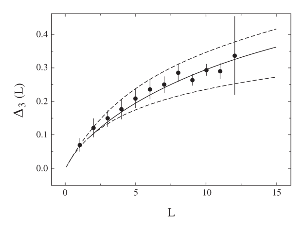
FIG. 20.: Experimental spectral rigidity $\Delta_{3}(L)$ in ²⁶Al. Solid dots represent the experimental results of the 100 levels between $0$ and $8$ MeV excitation energy. The solid line is the result of a numerical simulation of the random matrix model incorporating a symmetry breaking. This value of the symmetry breaking gave the best fit to the experimental data. For comparison the theoretical results for no symmetry and one fully conserved symmetry are shown as lower and upper dashed lines, respectively. Adapted from Ref. [137].

relatively large errors, the resulting rms Coulomb matrix element of about 20 keV agrees with the data mentioned above. In Ref. [228] a slightly different experimental analysis was presented. An interpretation in the framework of the RMT model for symmetry breaking is still possible. Due to the relatively large errors, the resulting rms Coulomb matrix did not change significantly. However, improved experimental data are highly desirable. Extensive shell–model calculations by Endt et al. [282] and Ormand and Broglia [243] which included the Coulomb interaction, yielded good agreement with both experiment and the statistical analysis. Very recently, Adams et al. [283] calculated the distribution of reduced transition probabilities in ²²Na using the shell model. Magnetic dipole ($M1$) and electric quadrupole ($E2$) transitions where studied among the first 25 states with positive parity, spin values ranging from $J=0$ to $J=8$, and isospin values $T=0$ and $T=1$. The results are consistent with a Porter–Thomas distribution. Remarkably, no dependence on spin, isospin, electromagnetic character or excitation energy was found.

The violation of parity conservation is modeled in the same way as isospin symmetry breaking. Naively, one might expect a very weak effect: The weak interaction is about $10^{-7}$ times weaker than the strong interaction. Whereas the spreading width of nuclear states due to the strong interaction is of the order of MeV, the spreading width for the weak interaction is, therefore, expected to be of the order of $10^{-7}$ eV. There are, however, two mechanisms which strongly enhance parity violation in the regime of isolated compound nucleus resonances [284, 285]. First, in this regime resonances of opposite parity have typical spacings $D$ of a few eV. A spreading width of $10^{-7}$ eV thus implies a rms weak interaction matrix element $V_{\rm weak}$ of about $10^{-4}$ eV and a ratio $V_{\rm weak}/D$ of about $10^{-4}$. This value is much larger than the naive estimate $10^{-7}$ and yields an enhancement factor of about $10^{3}$. Second, if an incident neutron populates a $p$ wave resonance which by parity violation is mixed with an $s$ wave resonance, decay of the latter by $s$ wave neutron emission is not hindered by the angular momentum barrier. Comparing this decay with the decay of the $p$ wave resonance back into the entrance channel, one obtains a second enhancement factor which is also about $10^{3}$. It is therefore not surprising that signals for parity violation amounting to several per cent were subsequently observed [286] in the helicity–dependence of neutron transmission through several $p$ wave resonances. A statistical analysis requires many such data, however. The TRIPLE collaboration has furnished and analyzed such a data base, see Refs. [287, 288]. The spreading width deduced from the data is of the order of $10^{-7}~{}{\rm eV}$, in agreement with theoretical expectations. We refer to a recent theoretical review on parity and time–reversal violation by Flambaum and Gribakin [289].

B Atoms and molecules

Complex atoms and polyatomic molecules are governed by the Coulomb interaction. The relevant energy scale is very different from the nuclear case: The ionization energies for atoms and the dissociation energies for molecules are of the order of several electron volts. In Secs. IV B 1 and IV B 2, we discuss atoms and molecules, respectively.

1 Atoms

It is not clear a priori whether atomic spectra are expected to show random matrix fluctuations. Complex atoms differ from nuclei in various ways. The nuclear charge $Ze$ is concentrated in the center. The mean–field approximation, the basis of the atomic shell model, is better justified and a better approximation than in the nuclear case. Nevertheless, the screened interaction between the electrons is not negligible. But is it strong enough to induce RMT behavior? Rosenzweig and Porter [82] seemingly were the first to investigate the fluctuation properties of spectra of complex atoms. This seminal work was done as early as 1960, only a few years after the first evidence for random matrix fluctuations in nuclear spectra had been found, see Porter’s review [9].

Rosenzweig and Porter analyzed spectra of neutral atoms, members of three chains. The first chain consists of the atoms Sc, Ti, V, Cr, Mn, Fe, Co, Ni with $Z=21,22,\ldots,28$, the second one of Y, Zr, Nb, Mo, Tc, Ru, Rh, Pd with $Z=39,40,\ldots,46$ and the third one of Lu, Hf, Ta, W, Re, Os, Ir, Pt with $Z=71,72,\ldots,78$. The levels were grouped according to parity $\pi$ and total angular momentum $J$. The angular momentum values ranged from $J=0$ to $J=17/2$. No data were available for Tc, Lu and Pt. In the three chains, there was a total of between 1000 and 2000 spacings for each parity. For each pair of $(J,\pi)$ values, the spacing distributions were analyzed in each of the three chains. For the odd parity levels, the first chain gave a spacing distribution close to Poisson, the third one a spacing distribution close to the Wigner surmise, and the second one an intermediate result, see Fig. 21. To explain their results, Rosenzweig

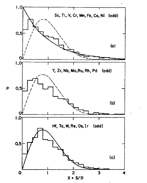
FIG. 21.: Nearest neighbor spacing distribution for the odd parity levels in the first, second and third chain (histograms (a), (b) and (c), respectively). Separate distributions were constructed for the $J$ sequences of each element and then the results were combined. For comparison, the Poisson distribution and the Wigner surmise are also drawn. Taken from Ref. [82].

and Porter used arguments related to the superposition of spectra, see Sec. III B 5. In the three chains, the sub–shells $3d$, $4d$ and $5d$, respectively, are filled. The chains differ in the strength of the spin–orbit force. In the first long chain, this force is very weak, and the Russell–Saunders or $LS$ coupling scheme applies. For larger $Z$ values, the spin–orbit force becomes stronger and the coupling scheme changes. In the second long chain, $LS$ coupling gives a relatively poor but still acceptable description. In the third chain, the coupling scheme is very different. In the first chain, $L$ and $S$ can be viewed as almost good quantum numbers. The spacing distribution for a given $J$ is a superposition of as many nearly independent spectra as there are $(L,S)$ pairs for that $J$, and the spacing distribution is very close to Poisson. This interpretation is strongly supported by an analysis which separates levels also by $L$ and $S$ quantum numbers. The ensuing spacing distribution is very close to the Wigner surmise. In the case of the third chain, there are no nearly conserved symmetries, and the spacing distribution is Wigner. In the intermediate case of the second chain, the symmetries are not completely destroyed yet. The picture differs for levels with even parity. For various reasons, the even parity spectra are simpler and closer to the ground state. To support their argument, Rosenzweig and Porter set up a random matrix model. For fixed $J$, they used a block–diagonal Hamiltonian. Each block represents a possible $(L,S)$ pair and is modeled by a GOE. The remaining matrix elements are independent Gaussian distributed random variables with rms value $\mu$. The spacing distribution was calculated numerically. As $\mu$ increases, the spacing distribution changes from Poisson to Wigner. The relevant parameter is $N\mu^{2}$, where $N$ is the matrix dimension. It was interpreted as the rms symmetry–breaking strength normalized to the mean level spacing, see Sec. III F.

We have discussed this work in some detail because in many ways it was a truly pioneering contribution. Aside from its technical aspects which later found application in many other papers, this work — and a preliminary study by the same authors — constitutes the first application of RMT outside the field of nuclear physics. It provided the first strong evidence for the universal applicability of RMT, independently of the specific interaction governing the physical system. In 1961, only a year later, Trees [290] extended this work by analyzing spacing distributions of calculated spectra.

In 1983, Camarda and Georgopulos [291] analyzed new level schemes of atoms in the beginning of the third chain, from La with $Z=57$ to Lu with $Z=71$, using the spectral rigidity and the covariance of adjacent spacings as observables. (For each pair of consecutive spacings, the latter is given by the expression (6)). This test of long–range correlations is also consistent with GOE predictions.

Of the more recent work, we only mention the extensive theoretical study of the rare–earth atom Ce by Flambaum et al. [292]. A realistic model is used to calculate the structure of complex atomic states. Above 1 eV excitation energy, these states acquire a structure similar to that of compound states in heavy nuclei (a linear superposition of very many basis states). Various spectral observables were worked out in this model and compared with GOE predictions.

2 Molecules

In a polyatomic molecule, there are three types of excitations: Electronic excitations, vibrations, and rotations. The energy scale of the electronic excitations is a few electron volt. Vibrational states built on top of every electronic state have an energy scale of 0.1 eV. On top of the vibrational states, there are rotational states with an energy scale of 0.1 meV. There is no spherical symmetry. The spectra are characterized by quantum numbers which differ from the ones used in atomic physics. Modern laser spectroscopy is capable of resolving the enormously rich and complex spectra of such molecules even at very high level density. Traditional theoretical techniques often fail in this regime, a description of individual levels is out of the question, and an analysis of the data with the aid of statistical concepts is called for.

The molecule NO₂ provides a particularly interesting example and has played a prominent role in the application of RMT concepts. Between the ground state and the dissociation threshold at about 3 eV, there are four electronic states. The Born–Oppenheimer approximation (based on an adiabatic separation of nuclear and electronic motion) breaks down in certain parts of the spectrum. It is this feature which makes NO₂ such an interesting object of experimental and theoretical studies of spectral fluctuations, although the molecule consists of only three atoms.

In 1983, Haller, Köppel and Cederbaum [293] studied experimental and theoretical vibronic spectra of the molecule NO₂ and of the acetylene kation C₂H${}_{4}^{+}$ in a regime where the Born–Oppenheimer approximation fails. Here, the term vibronic means that the excitation mechanism is only vibrational and electronic. Rotations are absent. Good evidence for GOE fluctuations was found in both the short– and long–range spectral observables. Zimmermann et al. [294] extended the analysis of NO₂ data, including a comparison of the measured intensity distribution with the Porter–Thomas law. Theoretical studies were presented by Zimmermann, Köppel and Cederbaum [295]. Leitner, Köppel and Cederbaum [296] compared the spectral statistics and the classical dynamics of both NO₂ and C₂H${}_{4}^{+}$. The dynamics of those systems with coupled potential surfaces can only approximately be described in classical terms since the electronic degrees of freedoms remain quantized. However, it turns out that the phase space is dominated by one of the potential surfaces. This allowed the authors of Ref. [296] to empirically establish a correspondence between this classical dynamics and the spectral fluctuation properties. In 1985, Mukamel, Sue and Pandey [297] investigated the spectral fluctuations and the distribution of resonance intensities in data on vibrationally highly excited acetylene. Deviations from the GOE predictions are attributed to missing levels. Sundberg et al. [298] extended this analysis of acetylene spectra.

It is apparent from this discussion that NO₂ has played a very important role in the investigation of spectral fluctuations in molecular physics. This was possible because the Grenoble group succeeded in improving the quality of experimental data substantially. Georges, Delon and Jost [299] have given a detailed account of the measurements on NO₂. They summarize the evidence for GOE fluctuations obtained from short– and long–range spectral observables as follows. The vibronic states built on the first and the second electronic state show GOE fluctuations. This can be attributed to the mixture of these states due the breakdown of the Born–Oppenheimer approximation. Higher up in the spectrum, GOE fluctuations occur for another reason in rovibronic states, i.e. in states where rotations on top of vibronic states become important. The mixing of these states is due to a symmetry breaking which has specific molecular physics causes. Very recently, parametric correlations as discussed in Sec. III H were addressed experimentally and theoretically in NO₂ by Nygård, Delon and Jost [300].

The correlation–hole method (Sec. III B 4) introduced by Leviandier et al. [74] brought a conceptually new aspect into the analysis of spectral fluctuations, see also the review [301]. This technique is designed for the analysis of raw spectra. It is less sensitive to the effect of missing levels than other observables. It does not require a line–by–line identification of the resonances. Hence, it can deal with the enormous amount of data supplied by modern laser spectroscopy. The correlation–hole method effectively separates the statistical fluctuations of the level positions and of the resonance shapes, see Fig. 22.

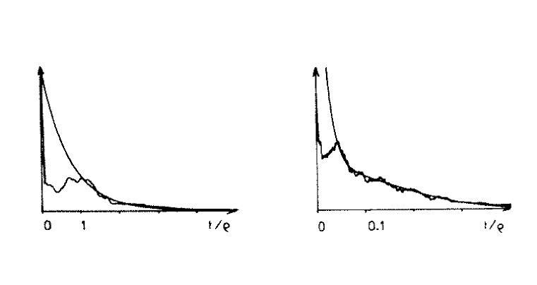
FIG. 22.: Correlation–hole analysis for a stimulated emission pumping spectrum of acetylene (left) and for an anticrossing spectrum of methylglyoxal (right). The properly smoothed decay function defined in Sec. III B 4 is shown. The variable $t/\rho$ should be identified with the variable $t$ of Sec. III B 4. The hole is due to the correlation of the level positions while the exponential decay is due to the resonance shapes. Notice the drastically different widths of the two holes, indicating a very different number of symmetries. Taken from Ref. [74].

Leviandier et al. applied this technique to anticrossing spectra of methylglyoxal. Consider a singlet state $|s\rangle$ populated from the singlet ground state $|s_{0}\rangle$. A triplet state $|t\rangle$ couples to $|s\rangle$ by some interaction $V_{st}$. If the energy difference between the two states obeys $|E_{t}-E_{s}|\gg V_{st}$, the interaction can be neglected and the resonance fluorescence light back into the ground state $|s_{0}\rangle$ attains a maximum. If, however, $|E_{t}-E_{s}|$ and $V_{st}$ are comparable, the admixture of the triplet state leads to a suppression of the fluorescence yield, since transitions from $|t\rangle$ to $|s_{0}\rangle$ are forbidden. The energy of the triplet states is shifted by a magnetic field $B$, and the resonance fluorescence yield $I(B)$ is measured as a function of $B$. For each isolated triplet state, $I(B)$ has Lorentzian shape. In methylglyoxal, there are many such triplet states with overlapping Lorentzians, and the measured resonance fluorescence intensity $I(B)$ has a complicated dependence on $B$. Leviandier et al. found a deep correlation hole in the decay function constructed from $I(B)$. The fluctuations of the anticrossing spectrum must therefore at least to some extent reflect GOE behavior. The exponential fall–off of the decay function is due to the Lorentzian shapes of the individual resonances. The arguments presented in Sec. III B 4 were used to conclude that the measured $I(B)$ must be a superposition of several non–interacting spectra. Further experimental work is due to Delon, Jost and Lombardi [75]. Pique et al. [302] applied the same type of analysis to spectra on acetylene. In the framework of scattering theory, a full–fledged random matrix model simulating these experiments was studied analytically [77] and numerically [80]. Detailed accounts of the correlation–hole method which also include other aspects of the statistical analysis were given by Lombardi et al. [78] and by Lombardi and Seligman [79].

The distribution of decay rates and related questions were investigated theoretically by Zimmermann, Köppel and Cederbaum [295], by Miller et al. [303] and by Peskin, Reisler and Miller [304], cf. also the work by Persson, Gorin and Rotter [253], see Sec. IV A 4.

Davis [305] introduced the interesting concept of hierarchical analysis: The structure of peaks in a spectrum is studied as a function of the resolution. In this way, hierarchical trees are generated which correspond to states of ever higher complexity. This analysis is intimately related to the constraints imposed by the experimental set–up and can yield significant statistical information. It seems worthwhile to see whether links can be established to RMT.

C General aspects

This short presentation of the evidence for random matrix fluctuations in many–body systems would be incomplete without a brief discussion of two questions posed by the results: (i) To what extent do the Gaussian ensembles properly model the properties of many–body systems? This question, asked in Sec. IV C 1, addresses the very foundations of the application of Random Matrix Theory to real systems. (ii) Are many–body systems chaotic? This question connects to the discussion of chaos in Sec. V and is treated in Sec. IV C 2.

1 To what extent do the Gaussian ensembles model many–body systems properly?

We recall that the distribution $P(H)$ for the Gaussian ensembles is uniquely derived from two assumptions: (i) $P(H)$ is invariant under orthogonal, unitary or symplectic transformations, respectively, and (ii) the independent matrix elements are uncorrelated random variables. There is evidence that both in atoms and in nuclei, the distribution of matrix elements differs from what is assumed in the Gaussian ensembles. The key argument is based on the observation that in both systems, the residual interaction is of two–body type. Thus, in a shell–model basis, the Hamiltonian matrix is sparse. Put differently, in an arbitrary basis, the elements of the Hamiltonian matrix are strongly correlated. In contradistinction, the Gaussian ensembles may be said to contain matrix elements of $k$–body type, with $k$ ranging all the way up to $N$. This is because in these ensembles, all matrix elements not connected by symmetry are uncorrelated. To what extend does this difference affect spectral fluctuations? The question can be formulated more precisely as follows. We consider a system of Fermions with a two–body [306, 307] and, more generally, a $k$–body random interaction. The matrix elements of the $k$–body operator between $k$–particle states are assumed to be independent Gaussian distributed random variables. There is evidence from nuclear physics [18] that for $k=2$, this is a realistic assumption. There are $m$ Fermions which occupy $N$ degenerate single–particle levels. Here, $k\leq m\ll N$. This defines the embedded Gaussian $k$–body ensembles [308]. Which are the spectral fluctuation properties of these ensembles? Very little is known analytically. This is why the embedded ensembles receive scarce attention in the present review. Numerical simulations [18] have shown, however, that the local fluctuation properties of the embedded two–body random ensembles do agree with RMT predictions.

The Gaussian ensembles do not only fail to take account of the two–body character of the residual interaction. They also misrepresent the actual distribution of the matrix elements in a non–shell–model basis. This is shown by work of Flambaum et al. [292] who investigated the distribution of the non–diagonal matrix elements of the Hamiltonian for the $J=4$ states of odd and even parity in Ce. The basis is given by all possible single–determinant states which are first constructed for a given value of the total azimuthal quantum number $M$ of the atom and then rotated such that the Hamiltonian is block diagonal in the total angular momentum $J$. These states are labeled by an index $n$. For $m\neq n$, Flambaum et al. found the empirical law

$$P(H_{nm})=C\frac{\exp\left(-|H_{nm}|/V\right)}{\sqrt{|H_{nm}|}}$$ (7)

where $C$ and $V$ are constants. For $m\simeq n$, a peak occurs on top of this distribution. Nonetheless, the spectral fluctuations calculated/measured in this atom agree with the GOE.

In spite of these shortcomings, the Gaussian ensembles generically model the fluctuation properties correctly. The reason is that fluctuations are studied on the unfolded, i.e. local, scale defined by the mean level spacing. This is in contrast to average or global properties which cannot be modeled by these ensembles. The local fluctuation properties are very insensitive to details of the distribution $P(H)$. For a class of ensembles, this is shown in Sec. VIII. More can be found in the review by Brody et al. [18]. This issues have received renewed interest in recent years, cf. the review by Flambaum and Gribakin [289] and the work of Müller and Harney [309, 310] and Granzow, Harney and Kalka [311].

2 Are many–body systems chaotic?

We have presented evidence to the effect that the complex structure of the many–body system often yields fluctuation properties which are consistent with RMT. There is also evidence for Poisson–type fluctuations, especially in systems capable of collective motion. In the description of these phenomena, we have tried to avoid the terms “chaotic” and “regular”, respectively, for these two scenarios. It is shown in Sec. V that for systems with few degrees of freedom, there is strong and growing evidence for the correctness of the Bohigas conjecture. As stated in the Introduction, this conjecture links classical chaos to the spectral fluctuations described by the Gaussian ensembles. Does this conjecture also apply to many–body systems? We are not aware of any arguments which would establish a link between many–body systems and classical chaos. Various studies have shown chaotic features of single–particle motion in realistic potentials, see Sec. IV A 4. Therefore, it is intriguing and may even be justified to think of complex many–body systems such as nuclei, atoms or molecules as chaotic. Such thinking must come to terms, however, with the existence of regular collective and single–particle properties in the same systems which may show up as gross structures at the very energies where the underlying fluctuations are of GOE type. Thus, a theoretical understanding of why RMT is so successful in many–body systems has yet to be found. The evidence we have at hand is either experimental or phenomenological. RMT was developed and used in the context of many–body physics long before the connection to classical chaos in few–degrees–of–freedom systems had been suggested. Thus, in retrospective, it is no surprise that phrases such as “unreasonable effectiveness” were used to characterize the predictive power of Random Matrix Theory in many–body physics.

V Quantum chaos

RMT originated in nuclear physics and was conceived as a statistical approach to systems with many degrees of freedom. However, RMT applies also to few–degrees–of–freedom systems with chaotic classical dynamics. This observation is of recent origin, and it forms the content of the present section. In 1984, Bohigas, Giannoni and Schmit [5] stated the famous conjecture: “Spectra of time–reversal invariant systems whose classical analogues are $K$ systems show the same fluctuation properties as predicted by the GOE.” We recall that $K$ systems are the most strongly mixing classical systems. The most unpredictable $K$ systems are referred to as Bernouilli systems. An alternative, stronger version of the conjecture, also formulated in Ref. [5], replaces $K$ systems by less chaotic systems provided they are ergodic. In both its forms, this conjecture is commonly referred to as the Bohigas conjecture. For systems without time–reversal invariance, the GOE is replaced by the GUE. In its original version, the Bohigas conjecture was stated without a reference to the semiclassical regime, i.e. to the limit $\hbar\to 0$. However, all attempts to proof the conjecture are based on some kind of semiclassical approximation, see Sec. V I.

We begin with a brief review of the historical development prior and up to the formulation of the Bohigas conjecture (Sec. V A). In Sec. V B, we briefly outline the main concepts of dynamical localization. We then turn to systems which were crucial to the development (billiards, the hydrogen atom in a strong magnetic field, and others). These systems form the first major part of the present section (Secs. V C to V G). Although representatives of mesoscopic systems, quantum dots are included here (Sec. V E) because they share many properties with billiards. The examples given and many others strongly support the Bohigas conjecture. This accumulation of convincing evidence has led to several attempts at establishing a theoretical link between classical chaos and RMT. These are reviewed in the second part of this section, i.e. in Secs. V H to V I. Lack of space forces us to present only the key elements of this discussion. In Sec. V H, we outline a hypothesis which has particular bearing on RMT. It concerns the way in which the structure of classical phase space influences quantum properties. Three approaches towards a formal proof of the Bohigas conjecture are presented in Sec. V I: Periodic orbit theory, a field–theoretic approach using the supersymmetry method, and a probabilistic argument based on structural invariance. In Sec. V J, a brief summary of the present section is given. There are many excellent reviews on classical and quantum chaos. With respect to classical and semiclassical aspects, we mention only, in the order of appearance, the books by Moser [312], Lichtenberg and Liebermann [313], Schuster [314] and Gutzwiller [108].

A Historical development

In its beginnings, the development of quantum chaos was strongly influenced by chemists who tried to understand simple molecules. The phenomenon of avoided level crossings was of particular interest. We follow partly the survey given by Robnik [315].

In 1929, von Neumann and Wigner [21] had shown that level crossings cannot occur in generic systems and that avoided crossings appear instead. Teller [316] stated the same theorem again in 1937. Percival [317] argued in 1973 that, in the semiclassical limit, the energy spectrum ought to consist of a regular and an irregular part reflecting the regular and irregular parts of classical phase space. In the early eighties Ramaswamy and Marcus [318], Berry [319]. Zaslavsky [51] and Marcus [320, 321] showed that level repulsion and avoided crossings are typical for non–integrable systems. Already in the late seventies and early eighties, Zaslavsky [322, 323, 51], Berry [324, 325, 50, 319] and Berry and Tabor [326] expected a drastic change in the spacing distribution to accompany the transition from integrability to non–integrability. In 1979, McDonald and Kaufman [48] published their pioneering numerical study of the quantum analogues of the classically integrable circular billiard and of the classically chaotic Bunimovich stadium. This work was closely followed by numerical work of Casati et al. [49] on the Bunimovich stadium. In these papers, the above–mentioned expectations came true. Further and improved evidence, also in billiard systems, was presented by Berry [50] and by Bohigas et al. [47, 5, 327]. All this work is reviewed in more detail in Sec. V C. The behavior of eigenfunctions near avoided crossings was simultaneously studied by Noid et al. [328, 168], Marcus [320, 321] and Ramaswamy and Marcus [318] who showed that the eigenfunctions are strongly mixed. According to McDonald and Kaufman [48] and Noid [328] this causes a random pattern of the wave functions whose nodal lines do not cross. In these papers, evidence was found that the low–lying eigenvalues and the corresponding eigenfunctions do not follow this pattern and have mainly regular features.

For small spacings, level repulsion was expected to lead to a spacing distribution proportional to $s^{\nu}$. Using geometrical arguments, Berry [50] suggested the value unity for the “critical exponent” $\nu$, in keeping with the Wigner surmise for the spacing distribution in time–reversal invariant many–body systems. Zaslavsky [51] related $\nu$ to the Kolmogorov entropy for the classical system. His work was a pioneering attempt to find a quantitative relationship between classical chaos and spectral fluctuations, although no convincing evidence for his assertion was found.

More formal arguments were used in the framework of statistical mechanics. Pechukas [172], Yukawa [329] and Nakamura and Lakshmanan [174] showed that the probability distribution of the energy eigenvalues of the “Pechukas gas” coincides with the GOE probability density. We do not follow this important line here because there is no easy link to chaos in few–degrees–of–freedom systems.

B Dynamical localization

Dynamical localization is a completely unexpected and novel feature of quantum chaos. In a classical system, driven by some external time–dependent force, the occupation probability in phase space spreads forever diffusively. Not so in the quantum analogue: After some characteristic time, the wave packet stops spreading in momentum space. This phenomenon is referred to as dynamical localization. It is “dual” to the localization in configuration space typical of disordered systems, see Sec. VI. The close relationship between both types of localization phenomena was discovered by Fishman et al. [330, 331, 332]. In both cases, there is quantum suppression of classical diffusion. The wave packet relaxes into a non–ergodic localized state. For the case of the kicked rotor, a step towards formally establishing the correspondence between both types of localization was recently made by using the supersymmetric non–linear $\sigma$ model [333], see Sec. VI D. A detailed account of dynamical localization was given by Casati and Chirikov [334, 335], see also Ref. [336]. We partly follow Ref. [334].

From a conceptual point of view, the study of wave functions is quite different from that of level statistics. Levels are eigenvalues of the Hamiltonian and can be studied experimentally. The spectral fluctuation properties of the quantum analogues of classically chaotic systems have accordingly received much interest, and they form the content of the bulk of the present section. The wave function $\psi$, on the other hand, is not an observable. Investigating the evolution of $\psi(t)$ in time $t$, one disregards all aspects of quantum mechanics related to the measurement process, and the collapse of the wave function. However, the wave function $\psi(t)$ obeys the Schrödinger equation, a deterministic equation. Thus, direct comparison of the time evolution of $\psi(t)$ with the dynamics of the corresponding classical system is useful. Some authors prefer to reserve the term quantum chaos for investigations conducted in this spirit.

It should be emphasized that quantum dynamical localization in classically conservative systems is due to quantum suppression of classically chaotic diffusion. Many semiclassical studies address questions such as scars around periodic orbits or similar phenomena which are often also referred to as localization. These two effects, however, should clearly be distinguished.

Two time scales govern dynamical localization. The relaxation time scale $t_{R}$ is proportional to the density $\rho_{0}$ of those eigenstates (quasi energy levels) which are admixed to the original wave packet at $t=0$. This is the time scale on which periodic orbit theory can be applied. The time scale $t_{e}$ is characteristic of the classical relaxation to the ergodic steady state. The quantity

$$\lambda=\sqrt{\frac{t_{R}}{t_{e}}}$$ (1)

is a measure for the ergodicity of the state. Shnirelman [337] argued that for $\lambda\gg 1$ the final steady state and all eigenfunctions are ergodic, and the Wigner functions are close to the classical microcanonical distribution in phase space. If, however, $\lambda\ll 1$, all states are non–ergodic, and their structure is governed by quantum mechanics.

On a very short time scale (which, according to the uncertainty principle, involves very high energies) the wave packet spreads quite like a classical cloud of particles in phase space would. Then quantum effects set in, the wave packet spreads in a manner not allowed by the constraints of Liouville’s theorem in classical mechanics, and eventually may stop spreading and remain in a non–ergodic localized state. To measure the size of localized states, Izrailev [67] introduced the entropy localization length

$$l_{h}=\exp(h)$$ (2)

where the entropy is given by

$$h=-\sum_{n}|\varphi(n)|^{2}\ln|\varphi(n)|^{2}\ .$$ (3)

Here, $\varphi(n)$ are the wave functions in momentum space. In various cases, the wave functions are exponentially localized, i.e. one has $\varphi(n)\rightarrow\exp(-|n|/l),\ |n|\rightarrow\infty$. In those cases, $l_{h}$ turns out to be close to $l$. The spacing distribution of localized states obeys, in the extreme case, the Poisson law whereas the Wigner surmise describes that of fully ergodic systems. Thus, the spacing distribution can give information about the degree of ergodicity and localization. Remarkably, it has been found in numerical studies that the repulsion parameter $\beta_{\rm eff}$ in Izrailev’s phenomenological crossover formula (80) can be approximated by

$$\beta_{\rm eff}=\beta\frac{l_{\langle h\rangle}}{l_{e}}$$ (4)

where $l_{\langle h\rangle}$ is the average of $l_{h}$ over all states and $l_{e}\geq l_{\langle h\rangle}$ is the maximal entropy localization length corresponding to ergodic states. As usual, $\beta$ labels the three symmetry classes. Another measure is the inverse participation ratio

$$\xi_{m}^{-1}=\sum_{n}|\varphi_{m}(n)|^{4}$$ (5)

which is related but not identical to $l_{h}$.

One of the first examples to show dynamical localization was the kicked rotor. Another case, which is experimentally accessible, is that of the hydrogen atom in a microwave field. Experimental results by Bayfield and Koch [338] led to a series of activities. Casati et al. [339] predicted localization effects in this system which were experimentally confirmed by Bayfield et al. [340]. We refer the reader to the review in Ref. [336]. Recently, these studies have been extended to the hydrogen atom in both magnetic and microwave fields by Benvenuto et al. [341].

C Billiards

A classical billiard consists of a point particle which moves freely in a compact domain of $d$–dimensional space and which is reflected elastically by the boundary of this domain. The energy and the modulus of the momentum of the particle are constants of the motion which, therefore, is determined by geometrical optics. Hence, the dynamics (regular, mixed, or chaotic) is the same for all energies. We restrict ourselves to $d=2$. This case was and is conceptually of great importance. Examples of integrable (regular) billiards are furnished by the circle and the ellipse. Among the many examples of chaotic billiards, two have received particular attention. The Sinai billiard consists of a square and an inserted concentric circle. The particle moves in the domain between square and circle. The Bunimovich stadium

FIG. 23.: Four important billiards: the Bunimovich stadium (top left), the Sinai billiard (top right), the Pascalian snail (bottom left) and the annular billiard (bottom right). To reduce the symmetries, these billiard have to be cut along the symmetry axes which are drawn as dashed lines.

is of oval shape and consists of two equally long sections of parallel straight lines which at both ends are joined by two semicircles. In the Sinai billiard, chaos is due to the defocusing effect of reflection at the inner circle. In the Bunimovich stadium, chaos arises because the straight lines destroy the rotation invariance of the two semicircles. Alternatively, chaotic dynamics can be attributed to an “over–focussing” effect in this geometry. Four important billiards are shown in Fig. 23. Sinai and Bunimovich [342, 343, 344] have shown that both billiards are fully chaotic and belong to the Bernoulli class, i.e. to the strongest form of chaotic dynamics. Mathematical aspects were discussed by Katok and Strelcyn [345]. Physics–oriented reviews on classical chaos in billiards can be found in the article by Bohigas et al. [47] and in Gutzwiller’s book [108].

The quantum analogue of a classical billiard is defined by the stationary Schrödinger equation with Dirichlet boundary conditions (the wave function vanishes at the boundary). Apart from factors, the Hamilton operator for a free particle is simply the Laplacean. Therefore, the problem is mathematically equivalent to determining the vibrations of a membrane. Independently of the connection to quantum mechanics, such and more general systems are of considerable interest and have been studied by mathematicians for a long time. For example, the Dirichlet condition may be replaced by the Neumann boundary condition (the normal derivative of the wave function vanishes at the boundary). In these systems, the smoothed part of the level density and the smoothed part of the cumulative density $\xi(k)$, see Sec. III B, show some very general features. As a function of the wavenumber $k$, $\xi(k)$ is given by

$$\xi(k)=\frac{A}{4\pi}k^{2}\mp\frac{L}{4\pi}k+C\ .$$ (6)

Here $A$ is the area and $L$ the length of the perimeter of the billiard. The constant $C$ describes curvature corrections, cusps and other topological properties. The minus and the plus sign in front of the perimeter term apply in the case of Dirichlet and Neumann boundary conditions, respectively. In the case of a particle of mass $m$ in a quantum billiard, the energy is $E=(\hbar k)^{2}/2m$. Formula (6) is valid for arbitrary geometries. The area term was found by Weyl [346] in 1911 and 1912, the perimeter term by Kac [347] in 1966. More general results for arbitrary linear boundary conditions were derived by Balian and Bloch [348], cf. also Ref. [349]. A review of the interesting history of these results can be found in Refs. [47, 108, 350].

We focus attention on the spectral fluctuation properties of quantum billiards. In sharp contrast to the level density, these properties depend sensitively on the shape of the boundary. The spectrum of a billiard can be unfolded very efficiently with the help of formula (6). To analyze the spectral fluctuations, it is important to use only levels which pertain to the same set of quantum numbers. This is done by removing all symmetries from the problem. The Sinai billiard, for instance, has four symmetry axes. One considers instead a billiard comprising 1/8th of the area. In the case of the Bunimovich billiard, a billiard of 1/4th of the area is considered, see Fig. 23.

McDonald and Kaufman [48] investigated numerically the spectrum of the circle, a classically integrable system. The results for the spacing distribution are shown in Fig. 24. Level clustering and degeneracies due to the absence of level repulsion could clearly be seen. The rectangle, also regular, was studied with comparably high statistics (more than 10 000 eigenvalues) by Casati et al. [351]. To avoid degeneracies, the squared ratio of the side lengths was chosen as an irrational number. Simultaneously, Feingold [352] performed similar numerical work. The spacing distribution probes correlations on the scale of up to three or four mean level spacings and agrees very well with the Poisson distribution. The spectral rigidity $\Delta_{3}(L)$ for the system considered agrees with the Poisson behavior $L/15$ only up to a critical value of $L\simeq 100$ and becomes constant for larger interval lengths $L$. The spectrum of the rectangle is fully random only on scales below this critical value. On larger scales non–trivial correlations appear which cannot be seen in the spacing distribution. Casati et al. [353] argue that such correlations occur generically in integrable systems. The very large number of levels needed to see this saturation of the spectral rigidity is often not accessible in numerical simulations, let alone experiments.

Chaotic billiards behave very differently. In their pioneering work of 1979, McDonald and Kaufman [48] calculated eigenenergies and eigenfunctions of the Bunimovich billiard numerically. They showed that the spacing distribution is of Wigner type and stressed the qualitative difference to the spacing distribution of the circle calculated in the same paper, see Fig. 24. McDonald and

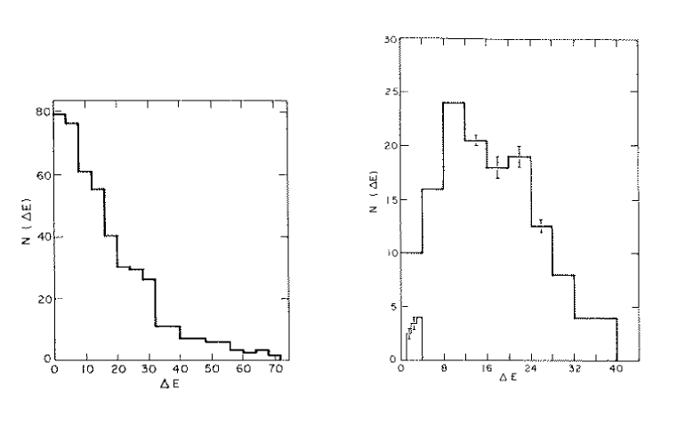
FIG. 24.: Nearest neighbor spacing distributions of odd parity levels in the circle (left) and the Bunimovich stadium (right). We notice that the spacing $\Delta E$ is not normalized to the mean level spacing and that the distributions $N(\Delta E)$ are normalized to the total number of spacings. The energy ranges are $2500<E<10000$ for the circle and $2500<E<4900$ for the stadium where the units are fixed by the choice $\hbar^{2}/2m=1$ in the Schrödinger equation. Taken from Ref. [48].

Kaufman related this difference to the classical integrability or non–integrability of the two cases. They also observed that the nodal lines of eigenfunctions in the Bunimovich stadium do not cross. The stadium was also investigated by Casati et al. [49]. Berry [50] studied the Sinai billiard in 1981, calculated about 500 eigenvalues and found linear level repulsion for small spacings. He gave a simple analytical argument for this behavior and mentioned the connection to RMT. Berry’s work demonstrates that accurate numerical methods for the calculation of a large number of levels are not only technically important, they often prompt new conceptual developments. In 1984, Bohigas et al. [5, 47] computed more than 700 eigenvalues of the Sinai billiard and found very good agreement of the spacing distribution with the Wigner surmise, see Fig. 4. This very accurate calculation provided the first statistically significant evidence of the validity of the Wigner surmise not only for small, but for all spacings. Bohigas et al. also showed that the spectral rigidity $\Delta_{3}(L)$ agrees very well with the GOE prediction up to $L\simeq 15$. Bohigas et al. [327] also calculated about 800 eigenvalues of the Bunimovich stadium and found the same excellent agreement of the data with GOE predictions. Mainly on the basis of these results, they formulated the famous conjecture quoted in the introduction to the present section. Beginning at that time, many more examples were studied numerically, comprising billiards and other systems with few degrees of freedom. Some of these cases are treated in other parts of this review. Most examples essentially support the conjecture, some mark its limitations.

The first study of the transition from regular to chaotic spectral fluctuations in a billiard is probably due to Robnik [315] in 1984. His billiard is defined by the conformal quadratic map $z^{\prime}=az+bz^{2}$ of the unit circle, described by the complex coordinate $z$. This is also referred to as the Pascalian snail, see Fig. 23. The parameter of interest is $\lambda=b/a$ with $0\leq\lambda\leq 1/2$. For $\lambda=0$ the billiard is integrable. For $\lambda=1/2$, a cusp occurs and the map is no longer conformal. For $1/4\leq\lambda\leq 1/2$, the classical billiard shows strong chaos [354]. The quantum analogue displays a transition [315] from Poisson to Wigner–Dyson statistics as $\lambda$ increases from $0$ to $1/2$. Robnik also introduced another billiard defined by the cubic map

$$z^{\prime}=\frac{z+bz^{2}+cz^{3}\exp(i\delta)}{\sqrt{1+2b^{2}+3c^{2}}}\ .$$ (7)

It is called the Africa billiard since for some values of the parameters $b$, $c$ and $\delta$, the shape resembles that of the continent Africa. Ishikawa and Yukawa [355] studied the transition from Poisson to Wigner–Dyson statistics in yet another billiard.

Of the numerous studies of billiards since 1984, we can mention but a few. A strong line of research uses semiclassical quantization and the theory of periodic orbits to investigate quantum properties of non–integrable billiards. Reviews are found in Refs. [94, 108, 350]. Sieber et al. [356] investigated the effect of the bouncing ball orbits on the spectral fluctuations of the Bunimovich stadium. The family of orbits which are perpendicular to the parallel straight sections has a strong effect, such that the long–range spectral fluctuations appear more regular. Sieber et al. constructed a semiclassical method to remove the contributions of these orbits from the spectral fluctuations. The general aspects of these effects had earlier been studied by Keating and Berry [357]. Bohigas et al. [358] introduced the annular billiard. It consists of the area between two circles with different radii, see Fig. 23. The billiard is integrable only when the circles are concentric. The properties of the system depend on two parameters, the ratio of the two radii and the distance between the two centers. The phase space is mixed. In the quantum system, tunneling from one regular region in phase space to another may be enhanced by the intermediate chaotic domain (“chaos–assisted tunneling”). This prediction of the Bohigas–Tomsovic–Ullmo model for mixed systems [154] has been confirmed analytically by Doron and Frischat [359]. Dittrich and Smilansky [360, 361] and Dittrich et al. [362] studied a chain of pairwise coupled billiards, with the aim to study localization, see also the review in Ref. [363]. The universal form of the curvature distribution (Sec. III H 1) was numerically confirmed for the Bunimovich stadium by Takami and Hasegawa [176], and for Robnik’s billiard defined above by Li and Robnik [181]. In the latter case, deviations for small curvatures from the analytical form (199) were attributed to peculiarities of the billiard. Tomsovic [109] studied parametric correlations in the Bunimovich stadium to investigate phase space localization properties of chaotic eigenstates. He introduced a correlator between state overlap intensities and level velocities. Tomsovic found sizable correlations due to scarring of specific states Those correlations are not described by RMT. Sieber et al. [364] discussed parametric statistics in billiards with mixed boundary conditions. Schanz and Smilansky [365] studied the Sinai billiard from a scattering point of view. They found good agreement of the spacing distribution of the eigenphases of the scattering matrix with Random Matrix predictions, see also the review in Ref. [366]. Primack and Smilansky [367] performed numerical simulations for the three–dimensional Sinai billiard. They found good agreement of the level statistics with RMT.

Pseudo–integrable billiards form a separate class, with specific fluctuation properties. A pseudo–integrable system is defined as a dynamical system whose phase–space trajectories live on surfaces with genus higher than one. The classical dynamics is not chaotic [368]. Billiards in the form of certain polygons fall into this class. Detailed studies of the spectral fluctuations in pseudo–integrable models can be found, for example, in the works of Richens and Berry [369], Cheon and Cohen [370] and Shudo et al. [371]. The spectral fluctuation properties of those systems have confusing features: on shorter scales, fluctuations properties such as the spacing distribution are often indistinguishable from the Wigner surmise. Only on longer scales, in the spectral rigidity for example, sizeable deviations from the properties of a chaotic system become visible. Balazs et al. [372, 373] introduced another class of billiards: These authors demonstrated that the free motion of a two–dimensional rigid body bouncing between two walls is equivalent to a billiard system. Thus, coin tossing can be viewed as a billiard problem. Billiards involving a non–Euclidean metric are of great interest for the problem of quantization. Schmit [374] has given a review on billiards on the hyperbolic plane. In chapter 19 of his book [108], Gutzwiller discusses the motion on a surface of constant negative curvature. The structure of wave functions can give rich information on the relationship between properties of the classical and the quantum billiard, see Heller’s review [375] and Gutzwiller’s book [108]. In some billiard systems, geometrical optics does not suffice to understand the motion. Examples are ray splitting effects [376], see Sec. V D 2, and Andreev billiards [333, 377, 378, 379] which prompted the introduction of new random matrix ensembles, see Sec. VI A 2. Recently, Borgonovi et al. [380] and Frahm and Shepelyansky [381, 382] studied localization effects of wave functions in billiards which partly destroy level repulsion. In such regimes, the fluctuations lie between Poisson and GOE. These authors studied diffusive effects in the Bunimovich stadium and rough billiards, respectively. Again, in the semiclassical limit $\hbar\to 0$, pure GOE statistics is found. This relates to the general discussion of dynamical localization in Sec. V B, i.e. to the quantum suppression of classically chaotic diffussion.

D Demonstrative experiments

The experiments discussed below show that billiards are not purely theoretical constructs but can be realized experimentally. For instance, quantum billiards can be simulated by microwave cavities. Such simulations are valuable because parameters such as the size and the shape of the cavity, the range of frequencies etc. can be altered, and they have been used to study specific aspects of quantum chaos. Simulations are not as fundamental, of course, as experiments on systems such as atoms, molecules, or nuclei where entirely new and unexpected phenomena may occur. Still, in some cases the simulation experiments exceed their original purpose and turn into interesting research objects of their own right. Moreover, some experiments (such as the ones on elastomechanical resonances in three–dimensional solids) open new frontiers: The wave equation and the boundary conditions in these bodies differs qualitatively from the Schrödinger equation.

The field was pioneered by Schröder [383] who, about 40 years ago and long before the connection to quantum chaos was established, realized the connection between acoustic waves and microwaves. He experimented with microwaves in order to study the acoustic properties of rooms. He used rectangular cavities and, interestingly, analyzed the nearest neighbor spacing distribution. For spacings larger than a mean level spacing or so, he found agreement with the exponential law now referred to as the Poisson distribution. He also discussed connections of his experiments with number theory. This and much more can be found in a fascinating book [384] he wrote on number theory in science and communication.

Demonstrative experiments with microwaves and elastomechanical waves are discussed in Secs. V D 1 and V D 2, respectively.

1 Microwave cavities

The stationary Helmholtz wave equations for the electric and the magnetic field $\vec{E}(\vec{r})$ and $\vec{B}(\vec{r})$, respectively, in a three–dimensional metal cavity read

$$(\Delta+\vec{k}^{2})\vec{E}(\vec{r})=0\qquad{\rm and}\qquad(\Delta+\vec{k}^{2})\vec{B}(\vec{r})=0$$ (8)

where $\vec{k}$ is the wave vector. If the boundary of the cavity is perfectly conducting, the tangential component of the electric and the normal component of the magnetic field vector vanish at the boundary. We consider a flat cavity formed by two plane, congruent and parallel metal plates. The cavity is uniform in the direction perpendicular to the planes, the $z$ axis. With $h$ the distance between the plates, modes with wave number $k<\pi/h$ cannot have a node in the $z$ direction and are therefore effectively two–dimensional. These modes are transverse magnetic, i.e. the electric field vector is parallel to the $z$ direction. For such modes, the relevant part of the wave equation reduces to a two–dimensional equation for the $z$ component of the electric field,

$$\left(\frac{\partial^{2}}{\partial x^{2}}+\frac{\partial^{2}}{\partial y^{2}}+k_{x}^{2}+k_{y}^{2}\right)E_{z}(x,y)=0\ .$$ (9)

The tangential component of $\vec{B}$ can be calculated from $E_{z}$. If we identify $E_{z}(x,y)$ with the wave function $\psi(x,y)$ and $k^{2}$ with $2mE/\hbar^{2}$, Eq. (9) becomes identical to the Schrödinger equation for a two–dimensional billiard. In the electromagnetic case, the ray limit is attained if the wave length is small compared to the dimension of the cavity. This corresponds to the classical limit in quantum mechanics.

Almost simultaneously but independently, Stöckmann and Stein [385] and Doron et al. [386] in 1990 published the first experimental studies of microwaves in such flat metal cavities and interpreted their results from the viewpoint of classical chaos. Stöckmann and Stein measured about 1000 eigenmodes of a Bunimovich stadium and of a Sinai billiard. Both cavities were about half a meter in size and 8 mm thick. The experimental spacing distribution agrees very well with the Wigner surmise. In a rectangle of similar size, Stöckmann and Stein obtained a Poisson distribution. Doron et al. investigated scattering in an “elbow” shaped cavity and compared the autocorrelation function of the scattering matrix versus frequency to a semiclassical formula [387] which predicts a Lorentzian shape. This shape applies when many channels are open. The autocorrelation function is non–Lorentzian in the case of few open channels [99, 388]. Lewenkopf et al. [388] improved the analysis of the data in the light of this fact. Doron et al. also discussed the enhancement of the Wigner time delay due to time–reversal symmetry. Another scattering experiment in microwave cavities was performed by Schultz et al. [389].

Sridhar [390], Sridhar and Heller [391] and Sridhar et al. [392] used a cavity to study wave functions of the Sinai billiard. To measure the distribution of the electrical field strength within the cavity, Sridhar et al. [392] used a perturbative technique. These authors demonstrated the connection between the wave functions and classical periodic orbits and identified scarred states predicted by Heller [375]. They also showed that a symmetry breaking in the Sinai billiard leads to localized eigenfunctions. Related experiments were simultaneously done by Stein and Stöckmann [393] in the Bunimovich stadium. The measured microwave power is proportional to the imaginary part of the Green function. The latter can be expressed semiclassically in terms of periodic orbits by Gutzwiller’s trace formula [108]. Thus, via Fourier transform, the measured power gives information about the classical orbits. Stein et al. [394] extended these investigations and thereby experimentally verified an insight due to Tomsovic and Heller [395, 396]. These authors had found that the semiclassical dynamics has a strong impact on the quantum mechanical behavior in billiards over very long time scales.

The statistics of wave functions was measured directly by Kudrolli et al. [397]. For the Bunimovich stadium, slight deviations from the Porter–Thomas law are caused by the bouncing ball orbits. The correlator of wave functions at different space points (see Sec. III E 2) agrees well with theoretical predictions for chaotic systems. Tiles in the cavity which act as hard scatterers change the cavity into a disordered system. Deviations from the predictions for chaotic systems due to localization effects are found both for wave function statistics and correlators. The results agree well with a formula by Fyodorov and Mirlin [398] which accounts for localization effects. Prigodin et al. [124] also compared experimental and theoretical results for wave functions, see Sec. III E 2.

All these experiments suffer from a broadening of the resonances due to absorption by the walls of the cavity. This makes it impossible to separate close–lying resonances. Missing levels pose a serious problem for the analysis of spectral fluctuations. To cure this problem, Gräf et al. [399] used superconducting niobium cavities at a temperature of 2 K. This results in a dramatic improvement of the resolution. About 1000 well resolved resonances were measured in the Bunimovich stadium. The effect of the bouncing–ball orbits (Sec. V C) is clearly visible in the spectral rigidity, and can be removed with the help of the semiclassical analysis of Sieber et al. [356]. With the same superconducting technique, Alt et al. [400] measured eigenmodes in the hyperbola billiard and compared the results with various transition formulae for the spectral fluctuations. Because of the high resolution, Alt et al. [401] could compare the shape of individual resonances with the Breit–Wigner formula and found excellent agreement over the full dynamical range. Likewise, Alt et. al [402] found good agreement of the distribution of partial widths with the Porter–Thomas law, see Sec. III E 1. These authors also confirmed the above–mentioned theoretical predictions of Lewenkopf and Weidenmüller [99] and Harney et al. [251] for the autocorrelation function of the scattering matrix in the limit of isolated resonances. The non–Lorentzian shape of this function implies that the Fourier transform decays algebraically and not exponentially. A detailed investigation of the decay properties of the Bunimovich stadium billiard was performed by Alt et al. [403].

Measurements of spectral observables at a crossover transition are particularly interesting. For the case of gradual breaking of time–reversal invariance, such experiments were conducted by So et al. [404] and Stoffregen et al. [405]. So et al. used a cavity with a thin ferrite strip adjacent to one of the walls. Time–reversal invariance is broken when a magnetic field is applied to the ferrite. In the $\Delta_{3}$ statistic, the GOE $\to$ GUE transition was observed with surprisingly good resolution. Stoffregen et al. placed a wave guide inside a microwave cavity. The wave guide contained a “microwave isolator” controlled by a magnetic field. One side of the cavity could be moved. This made it possible to study the motion of levels versus the length of the cavity. Stoffregen et al. determined the nearest neighbor spacing distribution, the tail of the curvature distribution of the eigenvalues, and the distance of closest approach at avoided crossings and found agreement of all three observables with GUE predictions. In an earlier study, Stöckmann et al. [406] had already shown experimentally that in the case of time–reversal invariance, the tail of the curvature distribution agrees well with theoretical predictions, see Sec. III H 1. A detailed theoretical study of microwave billiards with broken time–reversal invariance was given by Haake al. [407]. Recently, Kollmann et al. [408] and Stöckmann et al. [409] compared experimental results on the level motion with the predictions of the Pechukas gas [172]. They also study velocity and curvature distributions, see Sec. III H. Moreover, a link to periodic orbit theory is discussed.

Richter [410] discusses numerous further projects with microwaves: The Pascalian snail for the study of the regularity chaos transition, the annular billiard for the investigation of chaos assisted tunneling and experiments addressing localization.

In addition to the spectral rigidity, there exists another statistical observable, the correlation hole, to measure long–range correlations, see Sec. III B 4. The Fourier transform of the spectral two–point correlation function maps long–range properties onto short–range ones in Fourier space. For RMT correlations, this function has a hole at small values of the variable. Kudrolli et al. [411] found good agreement with the GOE prediction. Alt et al. [76] investigated the correlation hole in more detail, including an analysis of scattering data.

As early as 1991, Haake et al. [412] used microwave experiments to study a certain pseudo–integrable billiard, see Sec. V C. Shudo et al. [371] investigated pseudo–integrable billiards in the shape of polygons.

Cavities have been used also for another purpose. Cavities with simple boundaries show good agreement with the Weyl formula for the mean density of eigenvalues. This changes when tiles are placed within the cavity to roughen it. Deviations from the Weyl formula can be viewed as indicating a change of dimensionality [413]. In another study, Sridhar and Kudrolli [414] confirm experimentally the theorem of isospectrality. It states that pairs of billiards with different, but related, shapes exist which have identical spectra.

RMT was designed to describe fluctuation properties of quantum systems. Does it also work for the spectral fluctuation properties of other wave equations? Deus et al. [415], Alt et al. [416, 417] and Dörr et al. [418] studied the statistics of eigenmodes in three–dimensional microwave cavities. In a truly three–dimensional system, the vector Helmholtz equations (8) are structurally different from the scalar Schrödinger equation. Deus et al. found very good agreement of the spacing distribution with the Wigner surmise but deviations of the long–range correlations from the GOE prediction. They attributed the difference to a remnant of regularity in the irregularly shaped cavity. Alt et al. [416] used a more regular cavity and found statistics intermediate between Poisson and GOE even for the spacing distribution. Alt et al. [417] study a three–dimensional Sinai billiard. In both investigations, periodic orbit theory is applied and bouncing ball modes are extracted. The same geometry was investigated by Dörr et al. [418] who studied scarring and various statistical observables of the electromagnetic field distributions.

2 Acoustics and elastomechanics

Weaver [419] was the first author to study the question raised in the previous paragraph: Does RMT apply to the spectral fluctuations of wave equations different from the Schrödinger equation? In 1989, a year before the first microwave experiments were reported, he studied the elastomechanical eigenmodes of aluminum blocks. The motion of the displacement vector $\vec{u}(\vec{r},t)$ of a mass element at position $\vec{r}$ is governed by Navier’s equation [420]. For an isotropic material, the stationary wave equation [420] for the displacement vector $\vec{u}(\vec{r})$ can be decomposed into two Helmholtz equations for the longitudinal ($L$) and transverse ($T$) parts. These equations read

$$\left(\Delta+\frac{\omega^{2}}{c_{X}^{2}}\right)\vec{u}_{X}(\vec{r})=0\qquad{\rm for}\quad X=L,T\ .$$ (10)

Here $c_{L}$ and $c_{T}$ are the longitudinal and the transverse velocities, respectively, and $\omega$ is the frequency. Free boundary conditions (vanishing stress at the surface) apply. The longitudinal mode represents a pressure wave, the two transverse modes, shear waves. These modes are coupled through reflection at the boundary. Since always $c_{L}>c_{T}$, Snell’s reflection law leads to ray splitting: The reflection of an incoming longitudinal or transverse wave at the boundary yields both a longitudinal and a transverse wave traveling in different directions. This phenomenon is also referred to as mode conversion. Thus, elastomechanical wave equations are structurally very different from the Schrödinger equation and even more complicated than the wave equation for the electromagnetic field in three dimensions.

Weaver used rectangular aluminum blocks a few centimeters in size with angled slits. The slits break the symmetry of the blocks. Dropping steel balls onto the blocks and measuring the response, he found about 150 eigenmodes. The spacing distribution agrees well with the Wigner surmise, but the long–range correlations deviate from GOE statistics. Why are the results for these nearly regular blocks so close to GOE? Bohigas et al. [421] attributed this fact to the angled slits which act as defocusing structures. Delande et al. [422] used periodic orbit theory to analyze the problem and reached a similar conclusion. Weaver and Sornette [423] showed that these systems can be viewed as being pseudo–integrable. On short frequency scales, the correlations are indistinguishable from GOE predictions. These authors supported their conclusion by numerical simulations of a rectangular membrane with a point scatterer. Cheon and Cohen [370] reached a similar conclusion for polygons and pseudo–integrable billiards.

Using Weaver’s technique on brick–sized aluminum blocks, Ellegaard et al. [424] measured about 400 eigenmodes in the interval from 0 to 100 kHz. Rectangular blocks display Poisson statistics. The spectrum is a superposition of eight spectra pertaining to different symmetries. In such a case, Poisson statistics is known [23] to apply almost irrespective of the statistics of the individual spectra, see Sec. III B 5. Using blocks in the shape of a three–dimensional Sinai billiard, Ellegaard et al. observed the Poisson $\to$ GOE transition for the first time in a three–dimensional system.

Monocrystalline quartz blocks a few centimeters in size are even better suited objects because about 1500 eigenvalues can be measured [7] in the range from 600 to 900 kHz. Unlike aluminum, quartz is an anisotropic substance. Both the longitudinal and transverse velocities differ in the direction of different axes. Thus, the wave equation is even more complicated than Eqs. (10) which apply to isotropic materials. Quartz belongs to the discrete crystal group D₃. The rectangular blocks used by Ellegaard et al. [7] were cut in such a way that all symmetries are fully broken except a “flip” symmetry which has two representations, just like parity. The spectra were measured in transmission. The resolution was close to that of superconducting microwave cavities. The existence of the flip symmetry makes it possible to measure a gradual symmetry breaking which is statistically fully equivalent to the breaking of a quantum number such as parity or isospin [227, 137], see Secs. III F and IV A 5. The symmetry violation is achieved by removing successively bigger octants of a sphere from one corner, thereby again creating a three–dimensional Sinai billiard. The results for the spacing distribution are shown in Fig. 25. They are in agreement

FIG. 25.: Nearest neighbor spacing distribution $P(s)$ for the different radii $r$ of the removed octant: (a) $r=0$ mm, (b) $r=0.5$ mm, (c) $r=0.8$ mm, (d) $r=1.1$ mm, (e) $r=1.4$ mm, (f) $r=1.7$ mm, (x) a huge radius of $r\simeq 10$ mm. The dotted and the dashed curves are the theoretical predictions for a chaotic system containing no or one symmetry, respectively. Taken from Ref. [7].

with the random matrix simulations of Ref. [137]. The tiny symmetry violation induced by small octants immediately lifts all degeneracies. The spectral rigidity deviates from the GOE prediction. This is probably because the blocks used have features similar to those of a scalar pseudo–integrable system, see Sec. V C. On short scales, however, the spectral fluctuations are indistinguishable from RMT.

The experiments show that RMT applies far beyond quantum mechanics to classical wave equations which are very different from the Schrödinger equation. This is true even for anisotropic materials and for non–trivial effects such as crossover transitions. As Weaver points out in his original paper [419], statistical analysis has had a long history in acoustics, especially room acoustics and instrument calibration, see Ref. [425]. Vibrations of complex structures have likewise been analyzed for a long time with statistical methods [426]. We are under the impression, however, that Weaver was the first author to recognize the importance of RMT for the understanding of fluctuation properties in acoustics and elastomechanics. (Schröder’s work [383] addressed a regular system).

We turn to two–dimensional systems. Berry [50] cites unpublished experimental work by Ede on the vibrations of metal plates in the shape of a Sinai billiard. Sapoval et al. [427] investigated numerically and experimentally vibrations of membranes and found that fractal boundaries lead to localization effects. This is related to the work of Sridhar et al. [413] mentioned above. In 1992, Legrande et al. [428] studied numerically the flexural vibrations (bending modes) of thin metal plates in the shape of a Bunimovich stadium and extended in the $(x,y)$ plane. The stationary wave equation for the displacement $u_{z}(x,y)$ perpendicular to the plate is of fourth order and can be written as

$$(\Delta+k^{2})(\Delta-k^{2})u_{z}(x,y)=0$$ (11)

where $\Delta$ is the Laplacean in two dimensions. The wave number is given by $k^{4}=3\omega^{2}\rho(1-\nu^{2})/Eh^{2}$ where $\omega$ is the frequency, $\rho$ the density, $h$ the thickness, $\nu$ the Poisson number and $E$ the elasticity module. Longitudinal modes obeying the second order Helmholtz equation exist as well in elastic plates, but are not studied in Ref. [428]. Legrande et al. used the boundary condition of a clamped plate. Because of the form (11) the waves are a superposition of Helmholtz waves, and of exponentially decreasing and increasing solutions due to the operator $\Delta-k^{2}$. Nevertheless, the spectral fluctuations agree well with GOE predictions. Recently, Bogomolny and Hugues [429] calculated the smooth part of the cumulative level density, i.e. the Weyl formula, for flexural vibrations in elastic plates. They used a “semiclassical” approximation. Moreover, they worked out trace formulae for the integrable and the chaotic case.

Ray splitting occurs also in two–dimensional systems and causes problems similar to those of elastomechanics. Prange et al. [376] calculated the cumulative eigenfrequency density in a two–dimensional system with ray splitting. In three dimensions, the technical difficulties are such that the cumulative eigenvalue density of a solid with free boundaries has not yet been calculated. Dupois et al. [430] solved a simplified problem by introducing periodic boundary conditions.

E Quantum dots

During the last decade, it has become possible to manufacture microstructures of $\mu$m size. In the case of semiconductors, the electrons form a two–dimensional gas located between the two layers of a heterostructure. The potential confining this two–dimensional gas can be controlled extremely well, and it is possible to fabricate devices with widely varying shapes. At temperatures below 1 K or so, the phase coherence length is larger than the system size, and quantum coherence plays an important role. The elastic mean free path is typically $10~{}\mu$m or larger. The electrons move “ballistically”, i.e. they scatter only at the boundaries defined by the confining potential. The device can be viewed as a billiard. When coupled to external leads, it is called a quantum dot. The number of electrons on the dot varies typically between a few and several hundred. The coupling between dot and leads may be controlled by gates which create a potential barrier. A review of electron transport in quantum dots was recently given by Kouwenhoven et al. [431]. Here, we are concerned with level statistics and wave function correlations in ballistic quantum dots. In our discussion, we disregard the Coulomb interaction between electrons, save for the charging energy which is a mean field effect. Interaction effects in quantum dots have drawn interest only recently and are not discussed here, a detailed discussion was presented by Marcus et al. [432].

It is very useful to discuss quantum dots in the framework of scattering theory. Let $G$ denote the conductance and $\Lambda$ the total number of channels in each lead, defined by the number of transverse modes below the Fermi energy. The dimensionless conductance $g=(h/e^{2})G$ is the central object of theoretical interest. The Landauer formula

$$g=\sum_{a=1}^{\Lambda}\sum_{b=1}^{\Lambda}\left(|S_{ab}^{LR}|^{2}+|S_{ba}^{RL}|^{2}\right)$$ (12)

expresses $g$ as the total transmission. The latter can be written in terms of the scattering matrix $S$ describing the electron transport through the device. Here, $S^{LR}$ and $S^{RL}$ are those blocks of the scattering matrix $S$ which describe scattering from the left to the right lead and from the right to the left lead, respectively. A more detailed discussion of this formula is given in Sec. VI C 1. The dimensionless conductance $g$ is bounded by twice the number of channels in one lead, $g\leq 2\Lambda$. The properties of the dot depend on the strength of its coupling to the leads. Without barriers, we have $g\geq 2$. The electrons move freely between dot and leads, the quasibound states in the dot become strongly overlapping resonances, and $g$ shows conductance fluctuations. This regime is addressed in Sec. V E 1. For $g<1$ or so, the electrons must tunnel through the barriers between dot and leads, and $g$ displays isolated resonances. This “Coulomb blockade regime” forms the topic of Sec. V E 2.

1 Magnetoconductance and level correlations

In 1990, Jalabert et al. [433] suggested that fluctuations of observables such as the conductance might contain information about the shape of quantum dots. The spectral fluctuations of a regular system such as the circle differ qualitatively from those of a chaotic system such as the Bunimovich stadium. This difference might also affect the conductance fluctuations of quantum dots with either shape. It was known that magnetotransport properties in small two–dimensional conductors do depend on the geometry [434, 435, 436], and Doron et al. [386] investigated almost simultaneously the open “elbow” billiard with a similar aim, cf. Sec. V D 1. But Jalabert et al. established the connection between classical chaos and ballistic quantum dots. These authors investigated both semiclassically and numerically the fluctuations of $g$ versus an external magnetic field (“magnetoconductance fluctuations”). Jalabert et al. used the Landauer formula (12) and calculated semiclassically the autocorrelation function of $g$ versus magnetic field strength $B$,

$$c(B)=\langle\delta g(\overline{B}-B/2)\delta g(\overline{B}+B/2)\rangle$$ (13)

where $\delta g=g-\langle g\rangle$. The average is taken over an appropriate interval of values of $\overline{B}$. For a chaotic dot, they found

$$c(B)=\frac{c(0)}{\left(1+(eB/hc\alpha_{\rm cl})^{2}\right)^{2}}$$ (14)

where the constant $1/\alpha_{\rm cl}$ denotes the root–mean–square area enclosed by trajectories traversing the dot. The power spectrum (Fourier transform) of $c(B)$ decays exponentially,

$$s(\omega)=s(0)(1+hc\alpha_{\rm cl}\omega)\exp(-hc\alpha_{\rm cl}\omega)\ .$$ (15)

As mentioned in Sec. V D 1, Blümel and Smilansky [387] had computed a related quantity, the energy correlator of the scattering matrix, also semiclassically. The result (15) holds only for weak fields where the cyclotron radius is larger than the size of the dot. Moreover, the semiclassical approximation used in the derivation is justified only for large channel number, $\Lambda\gg 1$. Jalabert et al. compare formula (14) with numerical simulations in two classically chaotic scattering systems: a Bunimovich stadium with two external leads and a four disk junction. The latter consists of four identical disks whose centers form the corners of a square. The distance between these disks is a quarter of the disk radius. Thus the four disks form an open scattering system [437, 438], extending the famous three disk scattering system [439]. Good agreement is found. Deviations in the tail of the Lorentzian are ascribed to non–universal behavior due to short trajectories. Moreover, to check the uniqueness of their findings for chaotic systems, Jalabert et al. perform numerical simulations on a rectangle which is integrable. There are fluctuations, but the Fourier transform indicates that they are qualitatively different and have non–universal shape. Related theoretical work was presented by Doron et al. [98], Jensen [440] and Oakeshott and MacKinnon [441].

In 1992, Marcus et al. [442] performed an experimental

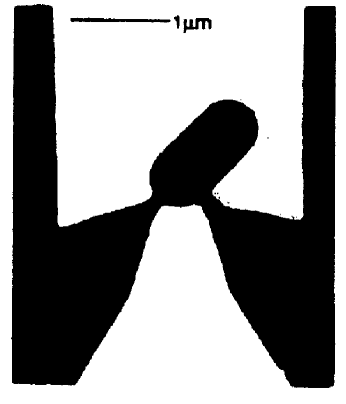
FIG. 26.: Electron micrograph of a quantum dot in the shape of a Bunimovich stadium, with $1~{}\mu$m bar for scale. This device was used in the experiments of Ref. [442]. The electrons can move in the black area. Two leads are coupled to the stadium. Adapted from Ref. [442].

test of the difference between regular and chaotic quantum dots. These authors fabricated two quantum dots in the form of a circle of radius $0.44~{}\mu$m, and two quantum dots in the shape of a Bunimovich stadium of length $1.2~{}\mu$m and width $0.6~{}\mu$m, see Fig. 26. All dots had the same area of $0.41~{}\mu{\rm m}^{2}$. Both the electron density of $3.8\cdot 10^{11}~{}{\rm cm}^{-2}$ and the mobility were measured and yielded an elastic mean free path of $2.6~{}\mu$m, several times the sizes of the dots, so that the electrons move ballistically. The power spectra show a striking difference for the two geometries. The semiclassical prediction (15) for chaotic motion agrees with the data for the Bunimovich stadium and not with those for the circle. The results are shown in Fig. 27.

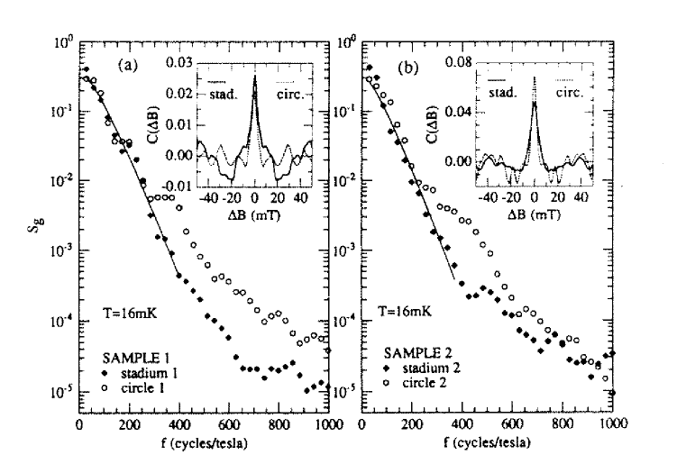
FIG. 27.: Averaged power spectra (here denoted by $S_{g}(f)$) of conductance fluctuations $\delta g(B)$ for stadium (solid diamonds) and circle (open circles) with approximately three transverse modes. The left and the right figures display the results for two different samples. Solid curves are fits of the semiclassical theory. The autocorrelation functions (here denoted by $C(\Delta B)$) of stadium (solid) and circle (dashed) are shown as insets. Taken from Ref. [442].

The number of channels in this experiment was rather small, $\Lambda\simeq 3$. Hence the semiclassical analysis is not very well justified. However, Marcus et al. provided convincing experimental evidence that, as Jalabert et al. had predicted, the difference between regular and chaotic motion reveals itself in the conductance fluctuations of quantum dots.

At zero magnetic field, the resistance displays sizeable peaks. The widths differ for the two geometries. At 20 mK, Marcus et al. found a few milli Tesla for the width of the peak of the Stadium and a much smaller value for that of the circle. A connection between these peaks and the weak localization effect [31] in disordered systems was suggested. Baranger et al. [443] investigated this phenomenon semiclassically. At zero magnetic field, the system is time–reversal invariant. The amplitudes which contribute to the reflection coefficient come in pairs. Semiclassically, the members of a pair correspond to time–reversed classical trajectories and interfere constructively. As the magnetic field is turned on and time–reversal symmetry is broken, the two amplitudes get out of phase. Hence at zero field, the reflection coefficient has a maximum and the transmission coefficient has a minimum. This leads to a maximum of the resistance. Baranger et al. showed that this weak localization effect depends on whether the dynamics in the dot is regular or chaotic. The calculation accounts for the existence of the peaks and for the difference in widths. The authors pointed out that the “diagonal approximation” [108] typically used in the semiclassical approximation (Sec. V I 1) does not yield all relevant contributions, in contrast to a full–fledged random matrix model such as that of Iida et al. [140].

In further experimental work, the weak localization dip of the conductance in the Bunimovich stadium was measured [444] for temperatures between 1.5 K and 4.25 K. In keeping with semiclassical arguments, the dip becomes less pronounced as the temperature increases, see also Ref. [445].

The experiments on chaotic quantum dots had shown that the shape of the weak localization peak is Lorentzian. Pluhar et al. [446, 89] reproduced this behavior in a random matrix model, using the random Hamiltonian approach to the scattering matrix as discussed in Sec. III D. The dependence on magnetic field was modeled as a GOE $\to$ GUE crossover transition. The fictitious time $t$ in Eq. (13) of Sec. II B is proportional to the square of the magnetic flux through the dot. In the notation of Sec. III F one has $t\propto\lambda^{2}$. Assuming ideal coupling to the leads, these authors obtain an exact expression in terms of a three–dimensional integral for $\langle g(t,\Lambda)\rangle$. Numerical integration shows that the expression

$$\langle g(t,\Lambda)\rangle\simeq\Lambda\,-\,\frac{\Lambda}{2\Lambda+1}\,\frac{1}{1+2(2\Lambda-1)t/\Lambda^{2}}$$ (16)

is an excellent approximation to $\langle g(t,\Lambda)\rangle$ for all $\Lambda\geq 2$. This expression has Lorentzian shape. Gerland and Weidenmüller [447] extended this calculation to the case of non–ideal coupling to the leads (barriers). They show that the peak shape is always Lorentzian but that the parameters depend sensitively on the transmission coefficients. Since electron–electron interaction is not included in this model, these results are not valid in the Coulomb blockade regime.

Using a Brownian motion model in the space of scattering matrices, Frahm and Pichard [448] and Rau [449] investigated the same problem, now formulated as a crossover transition from COE to CUE in the random $S$–matrix approach (cf. Sec. VI C). Frahm and Pichard calculated all correlators of of $g$ as functions of the eigenvalues of the transmission matrix and of a fictitious time $t$. Unfortunately, it has not been possible to relate $t$ with the flux through the dot. Moreover, the analytical dependence of $\langle g(t,\Lambda)\rangle$ on $t$ differs from Eq. (16). This suggests that the Brownian motion model in the space of $S$ matrices may not be a suitable means to model the crossover transition. This is in line with a difficulty often encountered in attempts to model parametric correlations in the random $S$ matrix (or transfer matrix) approach, cf. Sec. VI C.

The calculation of the correlator $c(B)$ of the magnetoconductance defined in Eq. (13) within a random matrix approach poses a much harder problem. Frahm and Pichard [448] point out that it is highly doubtful whether $c(B)$ can be worked out at all in the random $S$ matrix approach. Within an appropriate extension of the model of Pluhar et al., Frahm [450] calculated $c(B)$ using an asymptotic expansion in the inverse channel number $\Lambda$ and obtained the result (13). Recently, Gossiaux et al. [451] tackled the full problem for arbitrary channel number.

Prigodin et al. [116] investigated the conductance distribution $P(g)$ for a chaotic quantum dot weakly coupled to leads. The Hamiltonian has the form

$$H=H_{c}+\frac{i\alpha}{2\pi}\Delta+\frac{iV\Delta}{2\pi}\left(\alpha_{1}\delta(\vec{r}-\vec{r}_{1})+\alpha_{2}\delta(\vec{r}-\vec{r}_{2})\right)\ .$$ (17)

Here, $H_{c}$ is the disorder Hamiltonian of the chaotic dot. The second, non–Hermitean term on the right hand side of Eq. (17) accounts for incoherent processes such as electron–phonon scattering which produce a width $\overline{\Gamma}=\alpha\Delta/2\pi$ measured in units of the mean single–particle level spacing $\Delta$. Prigodin et al. focus on the regime $\Delta\ll\overline{\Gamma}\ll E_{C}$ where $E_{C}$ is the Thouless energy, see Sec. VI. In this regime, an interaction–free theory is appropriate. The last term on the right hand side of Eq. (17) describes [141] the coupling to the leads via point contacts at $\vec{r}_{1}$, $\vec{r}_{2}$ with $V$ the volume and $\alpha_{i},\ i=1,2$ dimensionless parameters. Prigodin et al. study this model with Efetov’s supersymmetry formalism. In the zero mode approximation and in the weak tunneling limit $\alpha\gg\alpha_{i},\ i=1,2$, they compute the moments

$$\langle g^{n}\rangle=\int P(g)g^{n}dg\ ,\qquad n=0,1,2,\ldots\ .$$ (18)

of the conductance. If the magnetic field is sufficiently large, weak localization effects can be neglected and the unitary symmetry class is appropriate. The distribution $P(g)$ decreases monotonically with $g$ and $g=0$ is the most probable value. This is in contrast to the case of systems strongly connected with leads. Prigodin et al. also re–derive the Porter–Thomas distribution for the unitary case, see Sec. III E 2. Marcus et al. [452] measured the magnetoconductance in the tunneling regime where the dot is nearly isolated. The power spectrum is enhanced at high magnetic frequencies. This is consistent with the results of Prigodin et al. [116]. Moreover, the magnetoconductance displays a crossover from aperiodic fluctuations at lower fields to periodic, Aharonov–Bohm–like fluctuations at higher fields. At the crossover point, the cyclotron radius of the electron motion has roughly the size of the Bunimovich stadium. For fields larger than this critical value, the electron bounces along the boundary of the stadium, and the motion becomes regular.

Baranger and Mello [453] and Jalabert et al. [454] used the random $S$ matrix approach to calculate statistical observables, particularly the distribution of the dimensionless conductance $g$. They discuss their results as functions of the channel number $\Lambda$ and the universality class $\beta$. In the case of only one channel in each of the two leads, they find

$$P(g)=\frac{\beta}{2}g^{\beta/2-1}$$ (19)

which shows a qualitative difference for the three cases $\beta=1,2,4$. With increasing channel number, $P(g)$ quickly approaches a Gaussian with non–zero mean. These results were obtained for ideal leads and for maximal coupling $\Gamma$ between dot and leads, and do not contradict those of Prigodin et al. Brouwer and Beenakker [455] bridged the gap between these two approaches by calculating, in the random $S$ matrix model, the distribution of $g$ for arbitrary $\Gamma$ and for all $\beta$. For $\beta=2$ and small $\Gamma$, the result of Prigodin et al. is reproduced.

2 Coulomb blockade regime and wave function statistics

In this regime, the barriers between dot and leads are so high that the intrinsic mean width $\overline{\Gamma}$ of the quasibound states in the dot is much smaller than the resonance spacing. The conductance is measured as function of the gate voltage applied to the dot. At low temperature, a series of well–defined isolated resonances is seen. Such measurements were made by Meirav et al. [456], Kouwenhoven et al. [457], McEuen et al. [458], Weis et al. [459] and Foxman et al. [460], see also the review by Kastner [461]. At each resonance, another quasibound level of the quantum dot passes through the Fermi surface from above as the gate voltage is increased, and the number of electrons on the dot increases by one. Beenakker [462] has shown that the resonance spacing $E_{n}-E_{n-1}+e^{2}/C$ is the sum of the spacing $E_{n}-E_{n-1}$ between adjacent quasibound single–particle levels in the dot, and the charging energy $e^{2}/C$. This charging energy suppresses tunneling processes between resonance peaks and causes the Coulomb blockade. For sufficiently small values of the capacity $C$, the charging energy dominates the expression $E_{n}-E_{n-1}+e^{2}/C$. In a plot of conductance versus gate voltage, equally spaced peaks appear. Several theoretical investigations [458, 462, 463] address the Coulomb blockade regime. Here we focus on a feature which is of particular interest for RMT. In many of the experiments [456, 458], the peak widths are dominated by temperature broadening, so that $\overline{\Gamma}\ll k_{B}T\ll e^{2}/C$, and all peaks have the same width. Nevertheless, the peak heights fluctuate by orders of magnitude. This behavior can be modeled within a random matrix approach. Several aspects of this problem are of general interest and are presented in Sec. III E. Here we discuss the applications specific to quantum dots.

We are interested in the regime $\overline{\Gamma}\ll k_{B}T<(E_{n}-E_{n-1})$. The height of a resonance peak is given by

$$g_{\rm max}=\frac{\overline{\Gamma}}{4\pi k_{B}T}\alpha\qquad{\rm with}\qquad\alpha=\frac{1}{\overline{\Gamma}}\frac{\Gamma^{(L)}\Gamma^{(R)}}{\Gamma^{(L)}+\Gamma^{(R)}}$$ (20)

where $\Gamma^{(L)}$ and $\Gamma^{(R)}$ are the partial decay widths of the resonance into the channels of the left and the right lead, respectively. RMT had been shown to give the correct description for the spectral fluctuations in irregularly shaped quantum dots. In 1992, Jalabert et al. [464] used RMT to determine the statistical properties of the quantity $\alpha$ in Eq. (20). For an asymmetric dot with a single decay channel per lead, the distribution function $P_{\beta}(\alpha)$ is obtained as

$$P_{1}(\alpha) = \sqrt{\frac{2}{\pi\alpha}}\exp(-2\alpha)$$ (21)

$$P_{2}(\alpha) = 4\alpha\Big{(}K_{0}(2\alpha)+K_{1}(2\alpha)\Big{)}\exp(-2\alpha)$$ (22)

for GOE and GUE, respectively. Here, asymmetric means that possible reflection symmetries have been removed by proper deformations of the system geometries. If such symmetries are present, one has $\Gamma^{(L)}=\Gamma^{(R)}$ and $\alpha=\Gamma/2\overline{\Gamma}$. Then the distribution function coincides with the Porter–Thomas law. In Eq. (22), $K_{n}$ is the $n$–th modified Bessel function of the second kind. Stone and Bruus [465, 466] performed extensive numerical tests of these results. They used the Africa billiard (7) as a model for the quantum dot and found good agreement with both of the predictions (22). Experimental verifications were presented by Chang et al. [467] and Folk et al. [468]. Stone and Bruus [465, 466] also computed the parametric velocity correlator (204) and showed its universality. This work was extended both analytically and numerically by several other authors [116, 115, 114]. Prigodin et al. [116] discuss to which extend their results can be applied to the Coulomb blockade regime. Bruus et al. [191] and Alhassid and Attias [469] studied parametric correlations (see Sec. III H 2) of the conductance peaks as a function of the magnetic field separation. They predict a squared Lorentzian in the case of fully broken time–reversal invariance. This was also experimentally verified in Ref. [468].

F Hydrogen atom in a strong magnetic field

The hydrogen atom in a strong magnetic field has played a central role in the conceptual development of quantum chaos. This is mainly due to three properties of this system. (i) It is a “real” system for which experimental data were available when theorists became interested in quantum chaos. (ii) Effectively, it has two degrees of freedom and is, therefore, calculable. (iii) It has an extremely useful scaling property which simplified the calculations and helped in the understanding of experimental results. Our brief discussion centers on the random matrix aspects of this system. Detailed presentations, particularly on the periodic orbit aspects, can be found in the reviews by Friedrich and Wintgen [470], Hasegawa et al. [471], and in Gutzwiller’s book [108]. A detailed discussion of the present status of experimental work on the hydrogen atom in magnetic and electric fields was recently given by Neumann [472].

The Hamiltonian of the hydrogen atom in a homogeneous constant magnetic field $B$ in $z$ direction reads

$$H=\frac{\vec{p}^{2}}{2m}-\frac{e^{2}}{r}-\omega_{L}L_{z}+\frac{1}{2}\omega_{L}^{2}(x^{2}+y^{2})$$ (23)

with $r=\sqrt{x^{2}+y^{2}+z^{2}}$ and where $\omega_{L}=eB/2mc$ is the Larmor frequency. The first two terms on the right hand side correspond to the Hamiltonian of the hydrogen atom without magnetic field. The third term represents the paramagnetic Zeeman contribution, the fourth one is the diamagnetic term. The last two terms break rotation invariance and destroy full integrability. With increasing magnetic field strength, ever larger parts of classical phase space become chaotic. We express the magnetic field in natural units defined by dividing the Rydberg energy $me^{4}/2\hbar^{2}$ by the Larmor energy $\hbar\omega_{L}$. Then, $B=\gamma\cdot 2.35\cdot 10^{5}{\rm T}$ where the magnetic field strength parameter $\gamma$ is dimensionless. We use atomic units. Because of axial symmetry with respect to the $z$ axis, the azimuthal quantum number $M$ is a good quantum number, and so is parity $\pi$. It is convenient to rotate the frame with the Larmor frequency $\omega_{L}$. This removes the paramagnetic term. In cylindrical coordinates, the momenta in $\rho=\sqrt{x^{2}+y^{2}}$ and $z$ direction are denoted by $p_{\rho}$ and $p_{z}$, respectively. For fixed $M^{\pi}$ values, the Hamiltonian reads

$$H=\frac{1}{2}\left(p_{\rho}^{2}+p_{z}^{2}\right)+\frac{M^{2}}{2\rho^{2}}-\frac{1}{\sqrt{\rho^{2}+z^{2}}}+\frac{1}{8}\gamma^{2}\rho^{2}\ .$$ (24)

Precise calculations which yield an excellent description of the experimental data were performed by various groups. As an example, we show results obtained by Holle et al. [473] in Fig. 28.

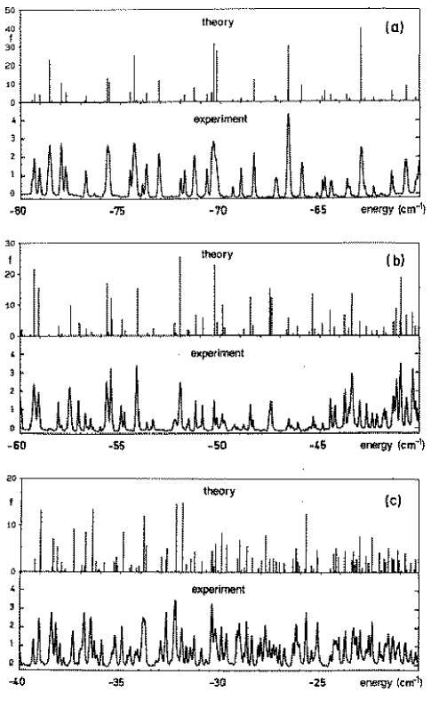
FIG. 28.: Comparison of theoretical and experimental results for the deuterium Rydberg atom. The magnetic field strength is 5.96 T. In spectroscopic units, the energies of the Rydberg states are between -80 cm^-1 and -20 cm^-1, where 1 cm^-1 corresponds to 0.12 meV. At the end of the energy range, i.e. above -25 cm^-1, the corresponding classical system becomes completely chaotic. Taken from Ref. [473].

The Hamiltonian (24) has the remarkable scaling property [474]

$$H(\vec{p},\vec{r},\gamma)=\gamma^{2/3}H(\gamma^{-1/3}\vec{p},\gamma^{2/3}\vec{r},1)\ .$$ (25)

Wintgen [475] and Wintgen and Friedrich [6, 476] realized that the scaling property (25) can be used for an efficient computation of the eigenvalues. This step was crucial. It was used later also by Holle et al. [477] for a much improved understanding of experimental data, see the review [470]. Wintgen and Friedrich [476] calculated the spectrum some meV below the ionization threshold at magnetic field strengths of a few Tesla. All properties depend only on the scaled energy $\varepsilon=\gamma^{-2/3}E$. This variable increases with both excitation energy and magnetic field strength. One has $\varepsilon<0$ for bound states and $\varepsilon>0$ for resonances. Between $\varepsilon=-0.8$ and $\varepsilon=-0.2$, the spacing distribution for bound states changes from Poisson to Wigner, see Fig. 5. In the same range, the fraction of classical phase space filled by regular trajectories decreases drastically. The coincidence of these facts strongly promoted the understanding of quantum chaos. As a function of $\varepsilon$ and for $L$ values below a critical value $L_{\rm max}$, the spectral rigidity follows the same pattern but saturates for $L>L_{\rm max}$. This is in agreement with Berry’s [56] general argument based on periodic orbit theory, see Sec. V I 1. The hydrogen atom in a strong field has been of great importance for the development of periodic orbit theory. Although the relevance of classical periodic orbits for the quantum spectrum was already known [478], Wintgen [479] was the first author to realize the full applicability of Gutzwiller’s theory. For reviews see Refs. [470, 471, 108].

Although a “real” system, the hydrogen atom in a strong magnetic field is intimately connected to one of the toy models studied theoretically. Upon the introduction of parabolic coordinates $\mu_{\pm}$ with $\mu_{\pm}^{2}=r\pm z$, the Hamiltonian (23) can be written as the sum of three terms. Each of the first two terms represents a harmonic oscillator with angular momentum barrier, while the third term provides a sixth order coupling in $\mu_{\pm}$ between the two. This is actually the form used by Delande and Gay [480] and Wintgen and Friedrich [470] to calculate eigenstates.

Simons et al. [481] verified the existence of universal parametric correlations, see Sec. III H 2, in the spectrum of the hydrogen atom versus magnetic field strength, see also Ref. [162]. These authors demonstrated the universality of the parametric level number variance and of the velocity correlator.

Zakrzewski et al. [482] made the following interesting observation. Very close to ionization threshold, the nearest neighbor spacing distribution deviates from the Wigner surmise. This is caused by an almost complete absence of spacings larger than about 1.5 mean level spacings. The classical motion is chaotic. However, the diamagnetic term in Eq. (24) confines the motion only in the $(x,y)$ plane. In the $z$ direction, the electron can move very far away from the proton. At such large distances, the Hamiltonian is the sum of two integrable parts. Zakrzewski et al. showed that this effect can be described by a regular Hamiltonian coupled to a chaotic one modeled by a random matrix.

G Model systems

Among a large variety of theoretical models, we subjectively select a few which, in our judgement, had impact on RMT. Regarding other systems, we refer the reader to the reviews by Bohigas [47, 350], Eckhardt [94], Gutzwiller [108], and Haake [57]. Molecular chemists introduced many such models systems which later became interesting for quantum chaos. In Secs. V G 1 and V G 2, we discuss coupled oscillators and the anisotropic Kepler problem, respectively.

1 Coupled oscillators

In 1973, Percival [317] predicted that, in the semiclassical limit, the energy spectrum of coupled oscillators consists of a regular and an irregular part which reflect the classically regular and irregular motion, respectively, see Sec. V A. To test this prediction, Pullen and Edmonds [483] in 1981 investigated numerically the classical and the quantum properties of two one–dimensional harmonic oscillators coupled by a fourth–order interaction,

$$H = H_{1}+H_{2}+4kx_{1}^{2}x_{2}^{2}$$ (26)

$$H_{i} = \frac{1}{2}(p_{i}^{2}+x_{i}^{2}),\qquad i=1,2$$ (27)

where $k$ is the coupling parameter. This system has several advantages over other model systems. For example, it is bound at all energies. Pullen and Edmonds studied the levels $E_{n}(k)$ as functions of the transition parameter $k$, and worked out the second differences

$$\Delta_{n}^{2}=|(E_{n}(k+\Delta k)-E_{n}(k))-(E_{n}(k)-E_{n}(k-\Delta k))|\ .$$ (28)

Large values of the $\Delta_{n}^{2}$’s are due to avoided crossings and occur in the regime where the classical dynamics is chaotic. Today we would say that $\Delta_{n}^{2}$ measures the curvature of the parametric level motion and indicates chaotic dynamics, see Sec. III H 1. Aside from their interest for chaotic systems, pairs of coupled harmonic oscillators became interesting also as models for a new class of integrable systems with a second hidden integral of motion [484, 485].

A year later, Haller et al. [486] studied the system (27) numerically. This system possesses a C_4v point–group symmetry. It also has a scaling property, and the levels can be computed efficiently. Haller et al. worked out the spacing distribution for a set of $k$ values and found a transition from Poisson to Wigner behavior which was fitted with the Berry–Robnik formula. The classical analogue of this system was known to undergo a transition from predominantly regular to chaotic motion. The work of Haller et al. was one of the first studies to show the close relationship between the transitions from regular to chaotic motion in classical mechanics, and from Poisson to Wigner–Dyson statistics in the quantum case. Meyer et al. [487] added further evidence in the frame of classical mechanics.

In a conceptually important contribution, Seligman et al. [488] investigated a related system which has a more

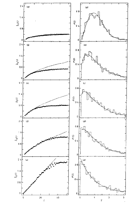
FIG. 29.: Numerically calculated spectral rigidities and nearest neighbor spacing distributions for the two coupled oscillators defined in Eq. (30). The parameters are $\alpha_{1}=0$, $\beta_{1}=122.1$, $\gamma_{1}=0$, $\alpha_{2}=0$, $\beta_{2}=24.1$, $\gamma_{2}=0$, $\alpha_{12}=0$, $\beta_{12}=-50\lambda$ and $\gamma_{12}=0$. The transition is studied as a function of the interaction strength $\lambda$. Figures (a) to (e) correspond to interaction strengths $\lambda=0.10,0.04,0.02,0.01$ and $0$. We notice the saturation of the spectral rigidities. The lines were obtained from a model of random band matrices. Taken from Ref. [488].

complex structure and shows richer features. They chose two one–dimensional oscillators with fourth–order potentials coupled by an interaction of the same form,

$$H = \frac{1}{2}(p_{1}^{2}+p_{2}^{2})+V_{1}(x_{1})+V_{2}(x_{2})+V_{12}(|x_{1}-x_{2}|)$$ (29)

$$V_{i}(x) = \alpha_{i}x^{2}+\beta_{i}x^{4}+\gamma_{i}x^{6},\qquad i=1,2,12\ .$$ (30)

The extensive numerical simulations show that, controlled by the parameters $\alpha_{i}$, $\beta_{i}$ and $\gamma_{i}$, the spacing distribution exhibits a transition from Poisson to GOE statistics when the classical system makes the related crossover from predominantly regular to chaotic motion. Seligman et al. also worked out the spectral rigidity and found a saturation beyond some interval length $L_{\rm max}$. Their results are shown in Fig. 29 for a certain choice of parameters. They also investigated the behavior of the corresponding classical system. Shortly thereafter, Berry [56] expressed the spectral rigidity in terms of periodic orbits and explained the saturation, see Sec. V I 1. To explain the transition, Seligman et al. also constructed a model of random band matrices. Very similar models are nowadays used in localization theory, see Sec. VI D.

Zimmermann et al. [489] calculated the spectral rigidity for the system (27) and compared the saturation effect quantitatively to Berry’s prediction. Berry argues that the maximal interval length $L_{\rm max}$ for universal GOE behavior is given by $L_{\rm max}=2\pi\hbar/DT_{\rm min}$ where $D$ is the mean level spacing and $T_{\rm min}$ is the period of the shortest periodic orbit, see Sec. V I 1. Zimmermann et al. found that this estimate is consistent with the tendency of the numerically obtained $L_{\rm max}$ as function of the coupling parameter.

Bohigas et al. [490, 491, 154] used two coupled quartic oscillators,

$$H=\frac{1}{2}(p_{1}^{2}+p_{2}^{2})+a(\lambda)\left(\frac{1}{b}x_{1}^{4}+bx_{2}^{4}+2\lambda x_{1}^{2}x_{2}^{2}\right)$$ (31)

with parameters $\lambda$, $b$ and $a(\lambda)$ as a model system to study the effect of classical transport on quantum properties. In a parameter range where the system is mixed, there exists a classical flux in phase space through imperfect barriers which are due to Cantori. Cantori are remnants of tori in the classical phase space of a mixed system. A semiclassical theory for the level number variance was derived and applied to this system by Smilansky et al. [492]. Because of its conceptual importance, we discuss this system and the concepts emerging from this study in Sec. V H.

2 Anisotropic Kepler problem

Another model system introduced by condensed–matter physicists is the anisotropic Kepler problem. The Hamiltonian is

$$H=\frac{p_{\rho}^{2}}{2m_{\rho}}+\frac{p_{z}^{2}}{2m_{z}}-\frac{e^{2}}{\sqrt{\rho^{2}+z^{2}}}$$ (32)

with $\rho=\sqrt{x^{2}+y^{2}}$. The anisotropy is caused by the difference between the masses $m_{\rho}$ and $m_{z}$. This model describes donor–impurity levels in semiconductors. In 1971, Gutzwiller [493, 494] had shown that the classical problem exhibits hard chaos. Later this problem became very important in periodic orbit theory. For most classical systems, the Kolmogorov–Arnold–Moser theorem prevents the abrupt transition from integrable to ergodic behavior: The structure of most invariant surfaces in phase space changes smoothly under small perturbations. However, this theorem does not apply to the pure Coulomb system. Therefore, it was not clear how the system (32) behaves if the mass anisotropy $1-m_{\rho}/m_{z}$ differs slightly from zero. Gutzwiller [495] had found strong evidence for an abrupt transition from regular to ergodic motion. His results and the question whether the spectral fluctuations change abruptly, too, led Wintgen and Marxer [496] to a detailed numerical study of the classical anisotropic Kepler problem and its quantum analogue. At a mass anisotropy of $0.2$, classical phase space is densely filled with remnants of tori, i.e. with Cantori. Thus, the system is only weakly chaotic. At sufficiently high excitation energies, the nearest neighbor spacing distribution agrees perfectly with the Wigner surmise. But the spectral rigidity follows the GOE prediction only up to an interval length of $L\simeq 7$ and then grows linearly with $L$ in a Poisson–like fashion. The speed of convergence to the GOE prediction is different in different regions of the spectrum. It is conjectured that the intermediate scale deviations and the slow convergence to the GOE predictions are connected to the pronounced Cantori structure of classical phase space. This example shows that, in its gross features, even a somewhat special system such as the anisotropic Kepler problem is consistent with the overall picture developed throughout this review: RMT type correlations become visible very quickly on short scales in the spectrum. On larger scales, however, there is stronger resistance to RMT correlations.

H Classical phase space and quantum mechanics

We now leave the discussion of special systems and return to the general aspects: The connection between quantum chaos and RMT. How does the structure of classical phase space manifest itself in quantum mechanics? About ten years ago, Berry and Robnik [138] conjectured that the spectrum of a mixed system should be a superposition of independent spectra, each associated with a chaotic (or regular) region in phase space. This is related to Percival’s [317] picture, see Sec. V A. Under the crucial assumption of independence of all these spectra, the nearest neighbor spacing distribution and other fluctuation measures can be predicted. In the simplest case, one obtains the Berry–Robnik formula for the spacing distribution (Sec. III B). In a more realistic picture, boundaries partitioning the chaotic part of classical phase space must be taken into account. Such boundaries may, for instance, be due to Cantori. Classical trajectories do pass such boundaries. Nevertheless, the existence of the boundaries defines a new time scale for the system. Bohigas, Tomsovic and Ullmo [154] extended the Berry–Robnik surmise by accounting for this time scale in terms of the classical flux through the boundary. The ensuing random matrix model acquires block structure. Each region of phase space is represented by a Gaussian or Poissonian ensemble, as the case may be. The corresponding matrix blocks are located on the diagonal of the total Hamiltonian matrix. The diagonal blocks are coupled through blocks of random matrices. The strength (second moment) of the latter is determined by the classical flux between the regions. The random matrix model for symmetry breaking (Sec. III F) is a special case of this model. The mathematical concept is very similar to early work by Rosenzweig and Porter on the spacing distribution in complex atoms, see Sec. IV B 1. In the model of Bohigas, Tomsovic and Ullmo, there exists, in addition to the coupling between different regions of the chaotic part of phase space due to classical flux, also a coupling between the regular and the chaotic blocks and among the latter which is due to quantum–mechanical tunneling processes. This relates to the idea of “chaos–assisted tunneling” (see Sec. V C) where separated regular regions in phase space are coupled via a chaotic region.

One can view the Bohigas–Tomsovic–Ullmo model as an extension of the original Bohigas conjecture: Since Cantori lead to more than one intrinsic time scale the ensuing random matrix model acquires a more complicated structure.

I Towards a proof of the Bohigas conjecture

The most remarkable feature of RMT is the prediction of universal statistical behavior of quantum systems. After the formulation of the Bohigas conjecture, it became a challenge to find analytical arguments linking classical chaos with RMT. Three approaches towards a formal proof of the Bohigas conjecture are presented here: Periodic orbit theory, Berry’s argument, and subsequent theoretical work (Sec. V I 1), a field–theoretic approach using the supersymmetry method (Sec. V I 2), and a group–theoretical and probabilistic argument based on structural invariance (Sec. V I 3). All three approaches involve, in one way or the other, a semiclassical approximation to quantum mechanics which links quantum and classical behavior, i.e. formally, the limit $\hbar\to 0$ is taken.

1 Periodic orbit theory

A natural framework for limking RMT and classical chaos is provided by periodic orbit theory. Developed by Gutzwiller [497, 498, 499, 493, 500] and by Balian and Bloch [501, 502], periodic orbit theory is based on the saddle–point approximation to Feynman’s path integral for $\hbar\to 0$ and is one of the means to implement the semiclassical approximation. In an important paper, Berry [56] used periodic orbit theory to investigate universal aspects of the $\Delta_{3}$ statistics (Sec. III B 3). We recall that $\Delta_{3}(L)$ is defined in terms of the staircase function $\widehat{\eta}(\xi)$. This function is the unfolded integral over the level density $\rho(E)$, and $\Delta_{3}(L)$ is obtained by minimizing the mean square deviation of $\widehat{\eta}(\xi)$ from a straight line over an energy interval of length $L$, see Eq. (83). Berry writes $\rho(E)$ as the sum of a smooth and a fluctuating part,

$$\rho(E)=\langle\rho(E)\rangle+\rho_{\rm fl}(E)\ .$$ (33)

The smooth part $\langle\rho(E)\rangle$ is identical to the mean level density $R_{1}(E)$, see Sec. III B 1. Periodic orbit theory can be used to write the fluctuating part as the sum over classical periodic orbits (“trace formula”),

$$\rho_{\rm fl}(E)=\frac{1}{\hbar^{\mu+1}}\sum_{j}A_{j}(E)\exp\left(\frac{i}{\hbar}S_{j}(E)\right)$$ (34)

where $j$ labels all distinct orbits, including multiple traversals. The phase factor in Eq. (34) is determined by the classical action $S_{j}(E)$ of the orbits. The amplitude $A_{j}(E)$ is related to the monodromy matrix of the orbit. In an integrable system, periodic orbits form $d-1$ parameter families filling $d$–dimensional phase–space tori. A chaotic system is defined as an ergodic system in which all periodic orbits are isolated and unstable. It can be shown that in Eq. (34), this implies $\mu=(d-1)/2$ for integrable and $\mu=0$ for chaotic systems. The length of the averaging interval needed for a separation of $\langle\rho(E)\rangle$ and of $\rho_{\rm fl}(E)$ must obey two conditions. (i) It must be small on the classical scale, i.e. small compared to the energy $E$ of the system. (ii) It must be large compared to two intrinsic energy scales of the system, the mean level spacing $D=1/R_{1}(E)$ and the energy $\hbar/T_{\rm min}$ given by the period $T_{\rm min}$ of the shortest periodic orbit. The associated energy $DL_{\rm max}=h/T_{\rm min}$ sets an important scale. Since $D$ is of order $\hbar^{d}$ and $T_{\rm min}$ is of order $\hbar$, we have $D\ll\hbar/T_{\rm min}$ in the semiclassical regime. The largest fluctuations in Eq. (34) stem from $\hbar/T_{\rm min}$. The energy range $DL$ is classically small, and we can write $S_{j}(E+\varepsilon)\simeq S_{j}(E)+\varepsilon T_{j}(E)$ where $T_{j}(E)=dS_{j}(E)/dE$ is the period of the orbit labeled $j$. Ignoring the $\varepsilon$ dependence of the amplitudes $A_{j}$ and of the mean level spacing $D$, the energy average in the definition (83) of $\Delta_{3}(L)$ can be performed trivially, resulting in a double sum over periodic orbits. Inspection of the energy scales allowed Berry to simplify the result further and to write it as an integral over all periods,

$$\Delta_{3}(L)=\frac{2}{\hbar^{2\mu}}\int_{0}^{\infty}\frac{dT}{T^{2}}\varphi(T)G\left(\frac{DT}{2\hbar}L\right)$$ (35)

where the function

$$\varphi(T)=\left\langle\sum_{i}\sum_{j,+}A_{i}A_{j}\cos\left(\frac{S_{i}-S_{j}}{\hbar}\right)\delta\left(T-\frac{1}{2}(T_{i}+T_{j})\right)\right\rangle$$ (36)

is the averaged double sum over the periodic orbit contributions. The plus sign in the sum over $j$ denotes the restriction to positive traversals, $T_{j}>0$. The function

$$G(y)=1-\left(\frac{\sin y}{y}\right)^{2}-3\left(\frac{d}{dy}\frac{\sin y}{y}\right)^{2}$$ (37)

does not depend on individual orbits $j$. The shape of $G(y)$ is very similar to (but $G(y)$ is different from) the two–level correlation function $X_{2}(r)$ of the GUE. Because of its shape, $G(y)$ selects from $\varphi(T)$ only those pairs of orbits whose average period exceeds $2\hbar/DL$. According to Berry, this feature reflects the fact that $\Delta_{3}(L)$ measures the deviations from the linear behavior of the staircase. Closer inspection of the steps leading to Eq. (36) shows that the linear behavior is determined by orbits with $T_{j}<\hbar/DL$ while the deviations are due to orbits with $T_{j}>\hbar/DL$. Berry then argues that the two–point function $\varphi(T)$ can be written in the form

$$\varphi(T)=\frac{\hbar^{2\mu+1}}{2\pi D}\left(1-b_{2}^{\rm sc}\left(\frac{DT}{h}\right)\right)\ .$$ (38)

Here $b_{2}^{\rm sc}(t)$ is the semiclassical approximation to the two–level form factor defined in Eq. (59) of Sec. III A 5, i.e. the Fourier transform of the unfolded two–level cluster function $Y_{2}(r)$. Collecting everything and introducing the dimensionless time $t=DT/h$ as new integration variable, one arrives at the semiclassical result

$$\Delta_{3}(L)=\frac{1}{2\pi^{2}}\int_{0}^{\infty}\frac{dt}{t^{2}}(1-b_{2}^{\rm sc}(t))G(\pi Lt)\ .$$ (39)

According to Eq. (39), the spectral rigidity can be obtained from a semiclassical approximation to the two–level form factor $b_{2}^{\rm sc}(t)$.

It remains to show that the semiclassical approximation to $b_{2}^{\rm sc}(t)$ leads to an expression for $\Delta_{3}(L)$ which is consistent with RMT. To this end, Berry uses sum rules. The first sum rule for the diagonal part of the sum in Eq. (36),

$$\varphi_{\rm dia}(T)=\left\langle\sum_{j,+}A_{j}^{2}\delta(T-T_{j})\right\rangle$$ (40)

is due to Hannay and Ozorio de Almeida [503]. The sum rule applies for large values of $T$. Periodic orbit theory shows that, in this limit, the density of periodic orbits increases, while the intensities $A_{j}^{2}$ decrease algebraically for integrable and exponentially for chaotic systems. Hence the limiting relations

$$\varphi_{\rm dia}(T)\longrightarrow\frac{1}{2\pi D}\left\{\begin{array}[]{cc}\hbar^{d}&\qquad{\rm integrable}\\ \hbar t&\qquad{\rm chaotic}\end{array}\right.$$ (41)

follow for large $T$ where $t=DT/h$ is the dimensionless time of the periods. The second sum rule due to Berry [56] says

$$\varphi(T)\longrightarrow\frac{\hbar^{2\mu+1}}{2\pi D}$$ (42)

in the regime $DT\gg\hbar$ or $t\gg 1$. This sum rule guarantees that the amplitudes and phases of very long orbits in the trace formula correctly generate the mean level density. Comparison with Eq. (38) shows that the second sum rule implies $b_{2}^{\rm sc}(t)\to 0$ for $t\gg 1$. This is equivalent to the vanishing of the two–level correlations on scales much larger than the mean level spacing.

One further ingredient from periodic orbit theory is still needed. It can be shown that for $T\gg T_{\rm min}$ and because of destructive interference, the diagonal sum (40) is a good approximation to the averaged double sum (36). We recall that $T_{\rm min}$ is the period of the shortest classical periodic orbit. In the regime $t_{\rm min}\ll t\ll 1$ where $t_{\rm min}=DT_{\rm min}/h$, the limit relations (41) of the diagonal sum can be used. In the case of integrable systems, the limit relation (41) coincides with the sum rule (42) implying that the diagonal approximation is also valid in the regime $t\gg 1$. Thus, $b_{2}^{\rm sc}(t)=0$ is a good approximation for the two–level form factor down to values of $t_{\rm min}$ and Eq. (39) yields

$$\Delta_{3}(L)=\frac{1}{2\pi^{2}}\int_{0}^{\infty}\frac{dt}{t^{2}}G(\pi Lt)=\frac{L}{15}\ ,$$ (43)

the random matrix result for Poisson regularity. For fully chaotic systems, the diagonal approximation must break down in the regime $t\gg 1$, because the sum rule (42) is in conflict with the limit relation (41). The off-diagonal terms enforce the physically required cutoff of the limit relation (41), expressed by $b_{2}^{\rm sc}(t)=0$ for $t\gg 1$. In order to work out the integral (39), Berry chooses a linear interpolation $1-b_{2}^{\rm sc}(t)\propto t$ for $t_{\rm min}<t<1$ as suggested by the limit relation (41), implying

$$\Delta_{3}(L)=\frac{1}{\beta\pi^{2}}\ln L+c_{\beta}$$ (44)

in the regime $1\ll L\ll L_{\rm max}=1/t_{\rm min}$. As usual we have $\beta=1$ and $\beta=2$ for time–reversal invariant and non–invariant systems, respectively. This logarithmic behavior is in agreement with the random matrix prediction (93) of Sec. III B 3. Berry also calculates the numerical values of the constants $c_{\beta}$. For $\beta=2$, he finds exact agreement with the GUE prediction. This is so because the linear interpolation coincides with the GUE result (68) for the two–level form factor. For $\beta=1$, there is no numerical agreement with the GOE prediction. This is because the GOE result (68) differs form the linear interpolation. Periodic orbit theory predicts universal behavior of the spectral rigidity only in the regime $L\ll L_{\rm max}$. Beyond this scale, the spectral rigidity saturates at a value $\Delta_{3}(\infty)$. Berry [138] works out $\Delta_{3}(\infty)$ and discusses examples.

It is very difficult to go beyond Berry’s semiclassical approximation to the two–level form factor, i.e. beyond the diagonal approximation to the periodic orbit double sum $\varphi(T)$. In some special, non–generic cases [504, 505, 506], and for the Riemann $\zeta$ function [507, 508], such a step has been possible. Recently, progress has been made by Bogomolny and Keating [509] in the general case. These authors use a relationship discovered by Andreev and Altshuler [510] to connect the non–diagonal contribution in the double sum (36) to the diagonal one. The key assumption is that in generic systems and modulo exact degeneracies, the orbits up to a cut–off period of the order of $h/D$ can be treated as statistically independent. Bogomolny and Keating point out that their results are closely related to the ones found by using the supersymmetric non–linear $\sigma$ model treated in the following section.

2 Supersymmetric field theory

We discuss two approaches [52, 53] based on semiclassical field theory. The central aim in both approaches is the same: To derive, within a semiclassical framework, a supersymmetric generating functional for conservative systems. For systems with fully chaotic classical phase space and in the long wave–length limit, this functional should yield RMT statistics for the eigenvalues. In addition, the derivation should display the limits of validity of RMT level statistics. Although based on a semiclassical approximation, both approaches avoid the use of periodic orbits or similar entities. The two approaches are technically demanding. Moreover, they touch upon difficult issues in ergodic theory and are still under discussion. Therefore, we restrict ourselves here to a discussion of the central ideas.

The approach by Muzykantskii and Khmelnitzkii [52], related to work by the same authors [511] discussed in Sec. VI E 3, starts from a disordered system and considers the limit of vanishing disorder. While it retains the usual semiclassical condition $k_{F}l\gg 1$ of Efetov’s supersymmetry approach (where $k_{F}$ is the Fermi wave number and $l$ the elastic mean free path), it does not use the long wave–length limit in its usual form, $ql\gg 1$. The wave number $q$ is typically given by the inverse of the linear dimension $L_{s}$ of the sample, and the paper focuses on the limit $l\gg L_{s}$. (In Sec. VI, the symbol $L$ is used for the sample size. Here we use $L_{s}$ to distinguish it from the symbol $L$ for the metric used in the supersymmetry method. Apart from this, we use the same notation as in Sec. VI.)

The authors consider a supersymmetric generating functional (averaged over disorder) of the form of Eq. (121). For a disordered system, the Lagrangean takes the form

$${\cal L}(\sigma)=\frac{\pi\nu}{8\tau}\int d^{d}r\ {\rm trg}(\sigma^{2})-\frac{1}{2}\int d^{d}r\ {\rm trg}\ln(-iK)$$ (45)

with $K=E-T-\lambda\sigma+\varepsilon L/2$, where $T$ is the operator of the kinetic energy and $L$ is the metric defined in Sec. III C 1. The source term is omitted. The authors circumvent the usual saddle–point approximation. Instead, they construct the Green function $G(\vec{r},\vec{r}^{\prime}|\sigma)$ of the operator $K$, a matrix–valued function in superspace. Let ${\tilde{G}}(\vec{r},\vec{p})$ denote the Wigner transform of $G$. Integrating ${\tilde{G}}(\vec{r},\vec{p})$ over the modulus $|\vec{p}|$ of the momentum $\vec{p}=\vec{n}|\vec{p}|$ defines a function $g_{\vec{n}}(\vec{r})$ for which a dynamical equation is derived. With $v_{F}$ the Fermi velocity, this equation reads

$$2v_{F}\vec{n}\frac{\partial g_{\vec{n}}(\vec{r})}{\partial\vec{r}}=i\left[\frac{\varepsilon}{2}L-\lambda\sigma,g_{\vec{n}}\right].$$ (46)

A functional $\Phi$ of $g_{\vec{n}}(\vec{r})$ is introduced with the property that the stationary points of $\Phi$ (with respect to a variation of $g_{\vec{n}}(\vec{r})$) are the solutions of Eq. (46). It is shown that in the limit $k_{F}l\gg 1$, the action of Eq. (45) can be rewritten in terms of the functional $\Phi$. This technically somewhat complex procedure allows taking the limit $k_{F}l\gg 1$ without implying $L_{s}\gg l$. Further confidence in the derivation stems from the fact that in the long wave–length limit, the resulting action ${\cal L}(\Phi)$ reduces to Efetov’s form, Eq. (126). Moreover, it is found that ${\cal L}(\Phi)$ remains well–defined in the limit $l\rightarrow\infty$. This suggests that in this limit, ${\cal L}(\Phi)$ yields the correct level statistics for systems without disorder. It is shown that for fully chaotic systems, limitations of the range of validity of Wigner–Dyson statistics are determined by properties of the classical Liouville operator.

The approach by Andreev et al. [53, 512] constructs a field theory where the effective action is associated with flow in classical phase space. Starting point is a supersymmetric generating functional containing the Hamiltonian operator $H$ for a system without disorder. A Gaussian average over energy centered at $E$ for the single system described by $H$ replaces the ensemble average typical for disordered systems. It leads naturally to the Hubbard–Stratonovich transformation, and to the introduction of the $\sigma$ matrix, see Sec. III C. The resulting Lagrangean is given by (we again omit the source terms)

$${\cal L}(\sigma)=\frac{1}{2}{\rm trg}_{\vec{q}}\sigma^{2}+{\rm trg}_{\vec{q}}\ln K$$ (47)

where $K=E-H-N\sigma+\varepsilon L/2$. Here, $\sigma$ depends on two sets of coordinates, ${\rm trg}_{\vec{q}}$ indicates a graded trace as well as an integration over both sets, while $N$ denotes the number of levels (eigenvalues of $H$) in the averaging interval. We note the formal similarity of Eq. (45) and of Eq. (47). A saddle–point approximation based on $N\gg 1$ leads to a saddle–point manifold and the occurrence of Goldstone modes. The resulting non–linear $\sigma$ model contains the classical Liouville operator. It is equivalent [53] to the model obtained in the zero disorder limit by Muzykantskii and Khmelnitzkii, although the two theories differ in form.

If $H$ is the Hamiltonian of a classically chaotic system, the non–linear $\sigma$ model requires regularization. This is achieved by adding a small noise to the classical Liouville operator. This procedure renders the classical motion irreversible. In the limit of vanishing strength of the noise, the spectrum of the resulting time–evolution operator (known as the Perron–Frobenius operator) reflects intrinsic irreversiblity properties of the underlying classical dynamics. The spectral properties of this operator determine the statistics of the eigenvalues of $H$. If the Perron–Frobenius operator describes an exponential relaxation towards equilibrium, then its spectrum has a gap between the lowest and the next eigenvalue, and the spectrum of $H$ displays Wigner–Dyson statistics in an energy interval determined by the size of the gap. Corrections to RMT can be obtained using the spectral properties of the Perron–Frobenius operator.

3 Structural invariance

In order to furnish the Bohigas conjecture with a formal justification, Leyvraz and Seligman [54, 55] take an alternative approach reminiscent of the use of probability theory in statistical mechanics. The three key steps of the argument are: (i) A given object is identified as a typical representative of some ensemble. (ii) This ensemble is known to have a particular property $p$ with probability one. (iii) As a member of the ensemble, the given object possesses property $p$ with probability one. Leyvraz and Seligman use this general probabilistic reasoning to establish a formal link between chaos and RMT. In this context, the three steps read: (i) A given classical system is identified as a typical member of a set $\Sigma$ of classical systems which can be embedded in an ensemble $E$. (ii) Upon quantization, the members of $E$ are known to possess random matrix fluctuations with probability one. (iii) Therefore, the given system also possesses random matrix fluctuations with probability one. We note that the term ensemble here has a meaning which differs from its use in RMT.

The set $\Sigma$ of classical systems is defined in terms of a number of characteristic properties common to all members of $\Sigma$. Such properties may be dynamical symmetries, behavior under time reversal, etc. The key concept in the construction of the ensemble $E$ is structural invariance. It is based on a group–theoretical notion. Let $G$ be the group of transformations which map a system in $\Sigma$ onto another such system. If $G$ possesses an invariant measure, then $G$ induces an invariant measure on $\Sigma$, and this defines the ensemble $E$. The properties defining $\Sigma$ must be ergodic, i.e. hold with probability one for any element of $E$.

Examples show that, in general, $G$ has infinite dimension and, therefore, does not possess an invariant measure. To overcome this difficulty, Leyvraz and Seligman consider systems with compact phase space $\Gamma$ and with phase–space volume $|\Gamma|$. The associated Hilbert space has finite dimension $N=|\Gamma|/h^{d}$ where $d$ is the number of degrees of freedom of the system. For systems without any discrete symmetries, invariant tori etc., i.e. for the fully chaotic systems, the elements of $G$ are given by the set $\Xi$ of all canonical maps of $\Gamma$ onto itself. According to an observation by Dirac [513], a unitary transformation can be assigned to every element in $\Xi$. Thus, $\Xi$ is mapped onto the unitary group $U(N)$ in $N$ dimensions. This group $U(N)$ possesses an invariant measure $d\mu(U(N))$ which is precisely the probability density of the Circular Unitary Ensemble (CUE). The third step is trivial and amounts to saying that quantization of any map $C$ in $\Xi$ yields the random matrix fluctuations of the CUE for the eigenphases of the quantum system. Leyvraz and Seligman also show that the inclusion of time–reversal invariance as a relevant property leads to the Circular Orthogonal Ensemble (COE). Moreover, they apply the same line of reasoning to time–independent Hamiltonians and obtain random matrix fluctuations for the eigenvalues of the quantum system. A critical discussion of the difficulties related to the construction of the ensemble $E$, the quantization procedure, and the necessity to consider a finite dimensional Hilbert space, is given in Ref. [55].

By constructing a surprising example, Leyvraz, Schmit and Seligman [514] show that in this approach, symmetries are easily dealt with. They consider a billiard in the shape of an equilateral triangle. It has three–fold rotation symmetry and three mirror symmetries with respect to the three symmetry axes. The mirror symmetries can be removed by a proper non–symmetric rounding of the edges. The resulting billiard still possesses the three–fold rotation symmetry. The system is time–reversal invariant. This suggests that the spectral fluctuations are described by the GOE. However, surprisingly, the GUE applies. Leyvraz, Schmit and Seligman [514] show this with the help of structural invariance. A semiclassical explanation was given by Keating and Robbins [515]: The characters of the corresponding symmetry group are complex which leads to phase contributions in the traces of the Green function in the irreducible representation. Formally similar to a breaking of time–reversal invariance due to an Aharanov–Bohm flux, this yields GUE statistics.

J Summary: quantum chaos

There exists overwhelming evidence that for fully chaotic systems governed by a single time scale, the Bohigas conjecture applies. A body of analytical arguments lends theoretical plausibility to this statement. However, a fully satisfactory proof of the conjecture is still lacking. For strongly chaotic systems with more than one intrinsic time scale (example: a chain of pairwise weakly coupled billiards, each fully chaotic), RMT in its pure form cannot apply. Such systems are kin to quasi one–dimensional disordered mesoscopic systems and possess the same statistical properties. A detailed discussion of such systems and their spectral statistics is given in Sec. VI. The situation is more difficult and less clear for the generic classical systems with mixed phase space. Here, the hypothesis of Sec. V H is likely to apply. However, a derivation of this hypothesis is lacking, and so is a non–phenomenological determination of the coupling between blocks.

VI Disordered mesoscopic systems

The investigation of disordered systems in one, two or three dimensions is almost exclusively a domain of condensed matter physics. The motion of electrons in a crystal with random impurities provides a key example. Particularly important for our purposes is the mesoscopic regime to which we will restrict ourselves in the following. In this regime, the phase coherence length $L_{\phi}$ is the largest length scale of the problem. Phase coherence is lost by inelastic scattering (in the case of electrons, through scattering by phonons or by other electrons), while elastic scattering does not destroy phase coherence. Thus, $L_{\phi}$ is essentially given by the inelastic mean free path. For electrons, $L_{\phi}$ grows strongly with decreasing temperature. For typical sample sizes $L$ in the $\mu$m regime (see Fig. 30), the condition $L_{\Phi}>L$ can be met at temperatures below $100$ mK or so. Here, quantum coherence is a dominant feature of experiment and theory. Closely related coherence phenomena occur when classical waves (light or sound) pass through a disordered medium. The theoretical treatments of phenomena in these different fields of physics bear a close analogy. Unless otherwise stated, we confine ourselves to the case of electrons.

Stochastic features enter into mesoscopic physics in two ways. The first source of randomness is provided by real spatial disorder. Schrödinger waves propagate through disordered media diffusively and/or show localization. Disorder is theoretically described in terms of a random disorder potential (see Eq. (14)) with a suitably chosen correlation length and probability distribution. Such stochastic modeling leads directly to a theoretical description in terms of an ensemble of Hamiltonians and constitutes a natural extension of classical RMT. The essential difference to the latter is due to the central roles played by dimension $d$, and by the spatial extension of the sample. The second, more implicit source of randomness arises from elastic wave reflection at suitably shaped boundaries which in the classical limit would lead to chaotic motion. For electrons, this situation is realized in “ballistic systems” where the elastic mean free path $\ell$ is larger than the sample size $L$. This source of randomness is the same as described in the preceding section. Again, dimension $d$ and spatial extension of the sample play a key role.

In Sec. III B 7 we have stressed the distinction between two averaging symbols, the angular brackets $\langle\ldots\rangle$ for spectral averages and the bar $\overline{(\ldots)}$ for ensemble averages. The equality of these two averages can be proven in certain cases, see Sec. III B 7. In many other cases, however, the equality of an experimental average (obtained by averaging over the spectrum, an external magnetic field, or the Fermi energy) and a theoretical ensemble average remains a hypothesis, cf. Sec. VI C 1. In this section on disordered systems we mainly use the symbol $\langle\ldots\rangle$ for average quantities, in spite of the fact that these quantities have typically been calculated by averaging over the random potential. In the few cases where we deal with a purely theoretical quantity which cannot be observed in an experiment (like, e.g., an average generating functional) we employ the bar.

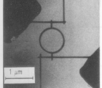
FIG. 30.: Picture of a mesoscopic gold loop taken with a scanning transmission electron microscope (STEM). Taken from Ref. [516].

For a systematic approach to the properties of spatially extended mesoscopic systems we have to consider various relevant length and energy (or time) scales. We assume that the Fermi energy $E_{F}$ is always the largest energy scale. The length scales $\ell$ and $L$ were defined above. A third important length scale is provided by the localization length $\xi$. Except for strictly one–dimensional samples, we always have $\ell<\xi$, and we assume in the following that $\ell\ll\xi$. Related to the two length scales $\ell$ and $L$ are two time (and corresponding energy) scales, the elastic scattering time $\tau=\ell/v_{F}$ and the time–of–flight $t_{f}=L/v_{F}$ through the sample, with $v_{F}$ the Fermi velocity. Further relevant energy (and related time) scales are the single–particle level spacing $\Delta$ at the Fermi surface and the Thouless energy $E_{C}=\hbar{\cal D}/L^{2}=\hbar t_{d}^{-1}$, where ${\cal D}$ is the diffusion constant and $t_{d}$ is the classical diffusion time through the sample. It was already remarked in Sec. II C that $E_{C}$ plays a central role in mesoscopic physics.

Four different regimes are distinguished.

(i) The localized regime with $L\gg\xi$. The system size exceeds the localization length, and the amplitude for propagation of an electron through the probe is exponentially small.

(ii) The diffusive regime with $\ell\ll L\ll\xi$. The system size is intermediate between the elastic mean free path and the localization length. Electrons are multiply scattered by random impurities and propagate diffusively. (Almost) all states of the system are extended and Ohm’s law applies. In this regime, we have a further inequality. The dimensionless conductance $g$ is given by $g=E_{C}/\Delta\gg 1$, see Eq. (17). Hence, we also have $\Delta\ll E_{C}$ and, moreover, $E_{C}\ll\hbar\tau^{-1}$ (this defines the diffusive regime). Thus, the diffusion time through the sample is too short to resolve individual levels but (trivially) long enough for the electron to be multiply scattered. The particular significance of the inequality $\Delta\ll E_{C}$ is discussed further below.

(iii) The condition $L\ll\ell$ or, equivalently $\tau^{-1}\ll t_{f}^{-1}$ characterizes both the ballistic and the nearly clean regimes. The system size is smaller than the elastic mean free path. The Thouless energy is replaced by the inverse time of flight $t_{f}^{-1}$ through the sample. The two regimes are distinguished by the degree of disorder.

(iii a) The ballistic regime where $\Delta\ll\hbar\tau^{-1}\ll\hbar t_{f}^{-1}$. The disorder, characterized by $\tau^{-1}$, is strong enough to thoroughly mix many energy levels of the system.

(iii b) The nearly clean regime where $\hbar\tau^{-1}\ll\Delta,\hbar t_{f}^{-1}$. The disorder is so weak that it can be taken into account by low–order perturbation theory.

All subsequent discussions of mesoscopic systems make use of this classification scheme. It should be evident already that the existence of four mesoscopic regimes vastly extends the range of problems dealt with in classical RMT. For instance, spectral fluctuation properties may differ in the four regimes. And the existence in $d>2$ of a mobility edge separating localized and extended states requires special attention.

In the following we discuss equilibrium (Secs. VI A and VI B) and transport (Secs. VI C, VI D, VI E, and VI F) properties of mesoscopic systems, respectively. Sec. VI A deals with the statistics of energy eigenvalues. Sec. VI B is devoted to persistent currents. Sec. VI C discusses the important case of quasi one–dimensional wires. This leads naturally to the investigation of random band matrices in Sec. VI D. In Sec. VI E we turn to systems in two and higher dimensions with special emphasis on the distribution function of conductance fluctuations in mesoscopic systems. Sec. VI F deals with the rather recent topic of two interacting electrons in a random impurity potential. Some concluding remarks are contained in Sec. VI G. We emphasize those facts, phenomena, concepts, and theoretical developments which are closely related to Random Matrix Theory in its widest sense. We pay special attention to the role of dimension, and of the spatial extension of the systems under study. We do so at the expense of a systematic introduction into and account of mesoscopic physics.

A Energy eigenvalue statistics

This and the following section are devoted to the spectral properties of isolated mesoscopic systems. Why has this topic found such wide interest? After all, transport properties have so far been the main source of experimental information on mesoscopic systems. And the study of the electrical polarizability of an ensemble of small metallic particles by Gorkov and Eliashberg [40] in terms of spectral correlations was a rather isolated occurrence.

The very strong interest in spectral fluctuation properties results from the intimate connection between transport properties and spectral properties of mesoscopic systems. In a seminal paper, this connection was pointed out already in 1977 by Thouless [517], see Sec. II C. His insight lies at the heart of the modern scaling theory of localization and helped to understand and interpret numerous mesoscopic fluctuation phenomena. Altshuler and Shklovskii [184] used the Thouless energy and a postulated connection to RMT to obtain a semiquantitative understanding of universal conductance fluctuations, one of the main manifestations of quantum coherence in mesoscopic systems. Finally, persistent currents in mesoscopic rings, which are the topic of Sec. VI B, measure the sensitivity of the spectrum to an external magnetic flux and provide a direct link between experiment and spectral fluctuation properties.

In Ref. [40], it was suggested that GRMT and Wigner–Dyson (WD) statistics in the form described in Sec. III A might be used to also address the spectral statistics in small disordered metallic particles at low temperatures. This suggestion could, however, not have been correct in general since WD statistics contains no parameter related to the dimensionality (or even the spatial extension) of the system. Research on spectral fluctuations in disordered metals has therefore to a large extent been driven by the following questions: Under which circumstances does WD statistics apply, where should one expect deviations, and how can these be calculated?

We approach the subject as follows. First, we recall in Sec. VI A 1 how the validity of WD statistics was established in the diffusive regime in some limiting case, and how corrections to this limit were calculated. Second, in Sec. VI A 2, we summarize attempts to go beyond diffusive systems, in the direction of both the ballistic and the localized regime. Third, we deal with spectral statistics in the proximity of the metal–insulator transition in Sec. VI A 3.

A recent review by Dittrich [363] nicely complements our discussion in the present section in that it focuses on the semiclassical approach to spectral statistics in (quasi) one–dimensional disordered systems.

1 Diffusive regime and Wigner–Dyson statistics

The above–mentioned conjecture by Gorkov and Eliashberg [40] was proved by Efetov [44]. Efetov showed that many statistical fluctuation measures of small disordered metallic particles can be calculated in terms of a functional integral over a field of supermatrices $Q(\vec{r})$. This “non–linear $\sigma$ model” was described in Sec. III C. For instance, the two–point correlation function $R(s)$ with $s=\omega/\Delta$ is – apart from an additive constant – given by

$$R(s)\propto{\rm Re}\int d[Q](\ldots)\exp\left(-S[Q]\right)$$ (1)

where (with $\hbar=1$)

$$S[Q]=-\frac{\pi\nu}{8}\int{\rm trg}\left[{\cal D}(\nabla Q)^{2}+2i\omega LQ\right]d^{d}r\ .$$ (2)

Here, $\nu=1/(V\Delta)$ is the density of states (with $V$ the volume and $\Delta$ the mean single–particle level spacing of the system), ${\cal D}$ the diffusion constant, $L$ a diagonal supermatrix, and $Q$ a supermatrix whose detailed structure depends on the symmetry class. The precise definitions can be found in Sec. III C, cf. also Ref. [44]. The quantity $\omega$ is the difference between two eigenvalues. The pre–exponential terms in Eq. (1) are not explicitly specified. They typically involve certain components of $Q$. In the context of Random Matrix Theory the correlation function $R(s)$ is typically denoted by $X_{2}(r\equiv s)$, see Eq. (55).

The “effective Lagrangean” $S[Q]$ comprises two terms, one with and one without spatial derivative. The gradient term owes its existence to spatial fluctuations in the $Q$ field and would disappear if the system under consideration were point–like. The second or “symmetry–breaking” term $\propto{\rm trg}[LQ]$ survives even in the zero–dimensional limit $Q(\vec{r})=Q_{0}={\rm const}$.

Efetov showed that in the zero–dimensional limit, his non–linear $\sigma$ model yields WD statistics for all three symmetry classes. He did so by reproducing the two–level correlation functions $R(s)$ of GRMT from the symmetry–breaking term of the non–linear $\sigma$ model. This result established the equivalence of the zero–dimensional $\sigma$ model and RMT (here in the narrow sense of the three Gaussian ensembles). Deviations from this limit are due to the spatial extension of the system.

To determine the range of validity of GRMT, one has to compare the energy scales associated with the two terms in $S[Q]$. For the gradient term this scale is given by the Thouless energy $E_{C}={\cal D}/L^{2}$, while the symmetry–breaking term is proportional to the difference $\omega$ of two eigenvalues. For $\omega\ll E_{C}$ the symmetry–breaking term gives the dominant zero mode, and one expects WD statistics, while for $\omega\geq E_{C}$ corrections to WD statistics should arise.

First corrections of this type were calculated by Altshuler and Shklovskii [184] within the perturbative approach of the impurity diagram technique. (We briefly turn to this method in our discussion of transport in quasi one–dimensional systems, see Sec. VI C). Their study was partly motivated by the phenomenon of universal conductance fluctuations, i.e. by the fact that the variance $\langle\delta g^{2}\rangle$ of the dimensionless conductance $g$ is of order unity in mesoscopic systems, see Sec. VI C 1. The argument by Thouless [517] (to which we have already alluded in the beginning of this section) linked spectral statistics and the statistics of the conductance through the relation $g=E_{C}/\Delta$. This relation is rewritten in the form

$$g=\langle N(E_{C})\rangle\ ,$$ (3)

where $\langle N(\omega)\rangle$ is the mean number of levels within an energy interval of size $\omega$. In the diffusive regime, where $\Delta\ll E_{C}$, we have $g\gg 1$ (good conductor). Through Eq. (3), the variance $\langle\delta g^{2}\rangle$ became linked with the number variance $\Sigma^{2}$ (see Sec. III B 3). Following common usage in much of the condensed matter literature we denote the number variance by $\langle\delta N^{2}\rangle$ in this section. Since Eq. (3) limits the spectral range of interest to the Thouless energy $E_{C}$, WD statistics seemed appropriate. However, WD statistics implies $\langle\delta N^{2}\rangle\propto\ln\langle N\rangle$, and the finite width of the energy levels due to the coupling to the leads had to be invoked [184] to reduce this value to $\langle\delta N^{2}\rangle\approx 1$ as required. For $\omega\gg E_{C}$ the result of the perturbative analysis in Ref. [184] was

$$\langle\delta N(\omega)^{2}\rangle=\frac{c_{d}k\tilde{s}^{2}}{\beta}\left(\frac{\omega}{E_{C}}\right)^{d/2}\ ,$$ (4)

where $c_{d}$ is a constant which depends on dimension $d$, where $\beta=1,2$, and $4$ for orthogonal, unitary and symplectic symmetry, respectively, where $k$ is the number of independent spectra considered, and where $\tilde{s}$ characterizes the degeneracy of the levels. This result shows that with increasing energy $\omega$, the stiffness in the spectra of disordered metals is reduced and the fluctuations in the number of levels increases. The physical picture behind these results is the following. For energies smaller than $E_{C}$, i.e. for time scales larger than the diffusion time through the sample, the wave packet of a diffusing electron has reached the boundary of the sample and is, in a sense, equilibrated. The spatial extension of the sample is then irrelevant and, therefore, WD statistics applies. This is precisely the same situation as in compound nucleus scattering, see Sec. IV A. In the opposite limit of energies larger than $E_{C}$ we deal with a wave packet that has not yet reached the boundaries of the sample. The corresponding level statistics has therefore not yet attained the universal limit and depends on the dimensionality of the system.

Numerically, the crossover to the regime described by Eq. (4) was observed by Braun and Montambaux [518], see Fig. 31.

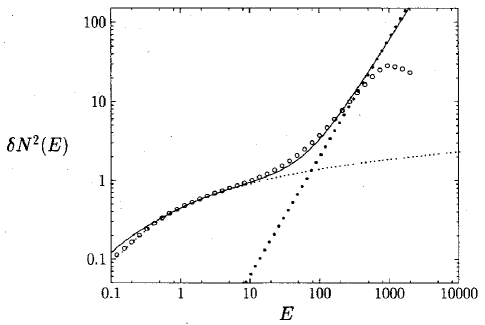
FIG. 31.: The number variance $\delta N^{2}$ for a system with $20^{3}$ sites versus the energy $\omega\equiv E$ in units of the mean level spacing (open circles). The Thouless energy is approximately $E_{C}\approx 2.5$. For comparison, the RMT behavior (dotted line), the asymptotic $E^{3/2}$ behavior of Eq. (4) (full circles), and the full perturbative result derived in Ref. [184] are also shown. Taken from Ref. [518].

The corrections found by Altshuler and Shklovskii [184] in the diffusive regime could be refined in later investigations, in particular by avoiding their perturbative analysis. Their calculation had focussed on the two–level correlation function $R(s)$ as a necessary prerequisite to determine the number variance. In the regime $1\ll s\ll g$, the perturbative approach [184] was only capable of yielding the smooth, non–oscillating behavior of $R(s)$. In two papers [519, 510], corrections to $R(s)$ were calculated in the non–perturbative framework of the non–linear $\sigma$ model. In the method used by Kravtsov and Mirlin, the parametrization $Q=T_{0}^{-1}LT_{0}$ for a constant $Q$ matrix was modified by the substitution $L\rightarrow\tilde{Q}(\vec{r})$ with an ensuing non–trivial change in the integration measure of the supersymmetric functional [520]. Fluctuations of $\tilde{Q}(\vec{r})$ around the origin $L$ of the coset space (leading to contributions from the gradient term in Eq. (2)) were taken into account perturbatively and were integrated out in the spirit of a renormalization group treatment, see Sec. VI E 2. For $g\gg s$ this led to the result

$$R(s)=1-\frac{\sin^{2}(\pi s)}{(\pi s)^{2}}+\frac{a_{d}}{\pi^{2}g^{2}}\sin^{2}(\pi s)$$ (5)

with $a_{d}$ a constant depending on dimension. Equation (5) holds for the unitary case. Expressions for orthogonal and symplectic symmetry are also given in Ref. [519]. The first two terms in Eq. (5) represent the result for the GUE, i.e. the universal limit. Since $g\approx E_{C}/\Delta$, see Eq. (3), the condition $g\gg s$ means $E_{C}\gg\omega$. Hence, the third term in Eq. (5) is a very small correction to the zero–dimensional limit of Eq. (2) originating from the comparatively massive modes of the gradient term. Therefore, corrections to the result of cRMT are quite small in the entire diffusive regime. The smooth part of Eq. (5),

$$R(s)=1-\frac{1}{2\pi^{2}s^{2}}+\frac{a_{d}}{2\pi^{2}g^{2}}\ ,$$ (6)

had already been found in the perturbative calculation [184].

Andreev and Altshuler [510] rederived Eq. (5) for $1\ll s\ll g$. They also showed that for $s\gg g$ the oscillations in $R(s)$ are exponentially damped and only the perturbative corrections of Ref. [184] survive. Their calculation was based on a new and interesting technical point. Following Ref. [510] we consider the generalization of Eq. (1) and Eq. (2) to parametric perturbations of the impurity potential characterized by the strength parameter $x$,

$$R(\omega,x) \propto \frac{\partial^{2}}{\partial J^{2}}\int d[Q]\exp(-S_{J}[Q])\Bigg{|}_{J=0}\ ,$$ (7)

$$S_{J}[Q] = -\frac{\pi\nu}{8}\int{\rm trg}\left[D(\nabla Q)^{2}+2i\omega LQ+iJLkQ-x^{2}\Delta(LQ)^{2}/2\right]\ .$$ (8)

The derivative with respect to $J$ produces the pre–exponential terms omitted in Eq. (1), and $k$ is a diagonal matrix with elements equal to $1$ and $-1$ in the Boson–Boson block and Fermion–Fermion block, respectively.

Let us focus attention on the case of unitary symmetry. The conventional treatment takes into account the usual saddle point $\propto L$ of the effective Lagrangean. There exists, however, one additional saddle point [510]. It has the form $-kL$ and is well defined for any finite non–zero $x$. This saddle point breaks supersymmetry and had previously been overlooked. Taking into account the contributions of both saddle points leads to Eq. (5). The orthogonal and symplectic cases could be treated similarly [510].

An interesting observation concerning the corrections to WD statistics for $s\gg g$ was made by Kravtsov and Lerner [521]. We recall that $s\gg g$ corresponds to $\omega\gg E_{C}$, i.e. to the limit in which Eq. (4) is valid. In this regime, the general (smooth) result for the two–point correlation function derived in Ref. [184] reads

$$R(s)=\frac{b_{d}}{\beta g^{d/2}|s|^{2-d/2}}\ .$$ (9)

But in two dimensions we have $b_{d}=0$, and the next order in $g^{-1}$ has to be invoked (weak localization corrections)! As a result, $R(s)$ for $d=2$ is given by

$$R(s)=\frac{\eta(g,\beta)}{\beta}\frac{1}{g^{2}}\frac{1}{|s|}\ ,$$ (10)

where $\eta(g,\beta)=(\beta-2)^{-1}$ for $\beta=1,4$ and $\eta(g,\beta)=-1/2g$ for $\beta=2$. Hence, in contrast to the number variance (4), the level correlation function was found [521] to be totally governed by weak localization corrections in this regime.

Motivated by the validity of WD statistics in the metallic regime, Akkermans and Montambaux [522] re–examined Thouless’ arguments [523, 517] connecting dissipation with level statistics, and the Thouless relation (3). (In the original work, the influence of WD statistics had not been taken into account, and this had meanwhile been found to be manifestly incorrect). Let the closed system with eigenvalues $E_{n}$ be subject to an external perturbation $\varphi$, and define the dimensionless quantity $g_{C}$ by

$$g_{C}=\frac{1}{\Delta}\left\langle\left(\frac{\partial^{2}E_{n}}{\partial\varphi^{2}}\right)^{2}_{\varphi=0}\right\rangle^{1/2}.$$ (11)

Obviously, $g_{C}$ measures the sensitivity of the levels $E_{n}$ to an external perturbation. (The perturbation can, for example, be realized by a magnetic flux $\phi$ with $\varphi=2\pi\phi/\phi_{0}$). Therefore, we may view Eq. (11) as a definition of the Thouless energy $E_{C}$ such that $g_{C}=E_{C}/\Delta$. The statement equivalent to Eq. (3) is then simply $g=g_{C}$ [523] where $g$ is the dimensionless conductance as given by the Kubo formula. Akkermans and Montambaux succeeded in deriving this “Thouless formula”. Using scattering theory, the Friedel sum rule, and very general assumptions concerning the number correlator $\langle\delta N(E_{F},\varphi)\delta N(E_{F},\varphi^{\prime})\rangle$, they could write $g$ in the form

$$g=-\frac{1}{4}\frac{\partial^{2}}{\partial\varphi^{2}}\langle\delta N^{2}(E_{F},\varphi)\rangle\Bigg{|}_{\varphi=0}\ .$$ (12)

Assuming WD statistics for the energy levels gave the central result

$$g\propto g_{C}\ .$$ (13)

Thus, the Thouless formula was derived in a much more rigorous fashion. In addition, it was found that [522]

$$\overline{\left\langle\left(\frac{\partial E}{\partial\varphi}\right)^{2}\right\rangle}^{\varphi}\propto\Delta\left\langle\left(\frac{\partial^{2}E}{\partial\varphi^{2}}\right)^{2}_{\varphi=0}\right\rangle^{1/2}$$ (14)

(with $E$ a typical energy level). The bar on the l.h.s. of Eq. (14) denotes an average over all flux values. We note that Eq. (14) connects a flux average with a local quantity at $\varphi=0$.

As the last item, we address the effect of time–reversal symmetry breaking in the diffusive regime. This problem arises in isolated mesoscopic rings threaded by a magnetic flux $\phi$. In Refs. [524] and [152], this problem was investigated and compared to the GOE $\rightarrow$ GUE crossover transition first considered by Pandey and Mehta [28], who analytically calculated all spectral correlation functions for a certain random matrix model, see Sec. III F 3. Dupuis and Montambaux [524] established numerically that the crossover transition is governed by the parameter $(E_{C}/\Delta)(\phi/\phi_{0})^{2}$. In the ergodic regime $\omega<E_{C}$, the transition is well described by the Pandey–Mehta random matrix model [28], see Eq. (13), provided the parameter $t$ used there is identified with the parameter $4\pi(E_{C}/\Delta)(\phi/\phi_{0})^{2}$. Altland, Iida and Efetov [152] calculated the two–point correlation function $R(s)$ in the crossover regime analytically. The calculation used the supersymmetry method and a novel parametrization of the $Q$ matrix, $Q=T^{-1}LT$, tailored to the breaking of time–reversal symmetry. The matrices $T$ were decomposed into two (Cooperon and Diffuson) parts,

$$T=T_{C}T_{D}\ ,$$ (15)

with

$$[T_{D},\tau_{3}]=0.$$ (16)

where $\tau_{3}={\rm diag}(1,-1)$ is the matrix which describes time–reversal symmetry breaking. With this construction, the symmetry–breaking term in the effective Lagrangean depends only on $T_{C}$. This fact simplifies the calculation considerably. As a result, the effective Lagrangean in the supersymmetric functional (1) for the correlation function $R(s)$ has the form

$$S[Q]=-\frac{\pi\nu A}{8}\int{\rm trg}\left[{\cal D}(\nabla_{x}-i(2\pi/L)(\phi/\phi_{0})[\tau_{3},Q])^{2}+2i\omega LQ\right]dx\ .$$ (17)

Here, $x$ is the longitudinal coordinate in the ring and $A$ the cross section of the ring. In the regime $\omega\ll E_{C}$, i.e in zero–mode approximation, an explicit result for $R(s)$ was derived, which coincides with the findings in Ref. [28].

This concludes our discussion of the diffusive regime. We have seen that in an energy range defined by the Thouless energy $E_{C}$, the spectral fluctuation properties (including the crossover induced by the breaking of time–reversal symmetry) are well described by the Gaussian ensembles. Deviations from this universal limit can be systematically calculated and are found to be generically small.

2 Ballistic and localized regimes

We summarize some important work on the crossover transition from the diffusive to either the ballistic or the localized regime, cf. the classification given at the beginning of this section. This crossover can be realized by changing either the system size or the strength of disorder. The extreme examples of a practically clean and a strongly localized system show that the regime chosen has a drastic influence on the level statistics. In the former case the levels are determined by the quantization conditions dictated by the boundary of the system while in the latter case the system is composed of essentially independent localization volumes, and level repulsion is suppressed.

Altland and Gefen [525] addressed the crossover from the diffusive to the ballistic regime. They studied non–interacting electrons in a two–dimensional square geometry with a random white noise potential. Within a suitable perturbative framework an equation for the two–point level correlation function $R(s;B_{1},B_{2})$ depending on two magnetic fields $B_{1}$ and $B_{2}$ was derived,

$$R(s;B_{1},B_{2}) = -\frac{\Delta^{2}}{2\pi^{2}}\partial^{2}_{\omega}\Bigg{(}{\rm tr}\Bigg{\{}\hat{\ln}[1-\zeta^{(D)}(\omega,B_{-})]$$ (19)

$$\qquad\qquad\quad+\hat{\ln}[1-\zeta^{(C)}(\omega,B_{+})]-S_{1}(\omega)\Bigg{\}}\Bigg{)}\ .$$

Here, $B_{\pm}=B_{1}\pm B_{2}$, $\hat{\ln}(1-x)$ is defined by the power series of $\ln(1-x)+x$, $S_{1}(\omega)$ is an essentially unimportant contribution and the coordinate representation of the (Cooperon and Diffuson) operators $\zeta^{(C,D)}$ reads

$$\zeta^{(D)}(\omega,B_{-};r,r^{\prime}) = \frac{\Delta}{2\pi\tau}G^{+}(E_{1},B_{1};r,r^{\prime})G^{-}(E_{2},B_{2};r^{\prime},r)\ ,$$ (20)

$$\zeta^{(C)}(\omega,B_{-};r,r^{\prime}) = \frac{\Delta}{2\pi\tau}G^{+}(E_{1},B_{1};r,r^{\prime})G^{-}(E_{2},B_{2};r,r^{\prime})\ ,$$ (21)

where $G^{\pm}$ are averaged single–particle Green functions. The spectral properties are entirely governed by the eigenvalues of the operators $\zeta^{(C,D)}$. Both the diffusive and the ballistic regime can now be investigated. In the diffusive regime, three energy ranges were considered, D1 ($0\leq\omega<E_{C}$), D2 ($E_{C}<\omega<1/\tau$), and D3 ($1/\tau<\omega$). It turns out that the range D1 coincides with the domain of WD statistics established in Ref. [44]. In the range D2, the results of Altshuler and Shklovskii [184] apply. These two cases have been treated in detail in the preceding section. In the range D3, we probe the dynamics of the system for times smaller than the elastic scattering time $\tau$. In this range the direction of the particle momentum is not yet completely randomized and the microscopic features of the random potential matter. For a standard Gaussian white noise potential the number variance was found to increase logarithmically,

$$\langle\delta N^{2}\rangle=\frac{1}{\pi}\left(\frac{L}{2\pi\ell}\right)^{2}\ln(E\tau)\ .$$ (22)

This result is non–universal since it depends on the details of the random potential. In the ballistic regime, the Thouless energy $E_{C}$ loses its physical significance because the electron typically traverses the sample non–diffusively. The extension of the sample enters the description now via the time of flight $t_{f}$ through the system. Again, three energy ranges were considered: B1 ($0\leq\omega<1/\tau$), B2 ($1/\tau<\omega<1/t_{f}$), and B3 ($1/t_{f}<\omega$). The range B1 corresponds to very large times. The electron traverses the system many times and is multiply scattered in the process. This range is therefore similar to the diffusive range D1. The range B3, on the other hand, corresponds to the case where the electron does not have the time to randomize its momentum or even to reach the boundary of the system. Therefore, B3 is analogous to D3. Finally, the range B2 is typical for the ballistic regime and has no analogue in the diffusive regime. Here, the electron has sufficient time to explore the whole system without undergoing complete momentum relaxation via scattering by the random potential. Therefore, the boundary of the system plays an important role. In the case of a two–dimensional square (or rectangle) [525] the number variance for the range B2 is given by

$$\langle\delta N^{2}\rangle=-\frac{2}{\pi^{2}}\ln(\gamma\tau)-\frac{2}{\pi^{2}}\frac{(E\tau)^{2}}{1+(E\tau)^{2}}\ ,$$ (23)

where $\gamma$ is a phenomenological level broadening of the order of $\Delta$. Interestingly, in this regime the fluctuations in the level number decrease upon increasing the energy window $E$. A discussion of both, the difference between energy– and disorder–averaging in ballistic systems, and the effect of finite magnetic fields is also contained in Ref. [525].

Another interesting point was made in Ref. [526]. There, it was shown that several observables are still characterized by the Thouless energy $E_{C}$ in the ballistic regime, although this energy scale can no longer be interpreted as the inverse transport time through the sample.

Building on ideas by Oppermann [527], Altland and Zirnbauer showed [333, 379] that new universality classes arise in mesoscopic structures with normally conducting–superconducting (NS) interfaces. They found that the ergodic limit of a quantum dot in contact with superconducting regions (cf. regimes D1 and B1 above) is not characterized by the three Gaussian ensembles GOE, GUE, and GSE, which define WD spectral statistics. Instead, the NS system is described by four new ensembles dubbed C, D, CI, and DIII after the associated four symmetric spaces in Cartan’s classification scheme, see Ref. [528]. These four ensembles correspond to the four possibilities of combining good or broken time reversal invariance with good or broken spin rotation invariance. Shortly after Ref. [333] became available a microscopic model for class C was derived by Frahm et al. [377]. To justify their claims the authors of Refs. [333, 379] started from the Bogoliubov–de Gennes Hamiltonian

$${\cal H}=\left[\begin{array}[]{cc}h&\Delta\\ -\Delta^{*}&-h^{T}\end{array}\right]$$ (24)

with the diagonal block $h_{\alpha\beta}=h^{*}_{\beta\alpha}$ and the pairing field $\Delta_{\alpha\beta}=-\Delta_{\beta\alpha}$. Depending on the symmetry class considered, further constraints on $h$ and $\Delta$ are necessary. With the two additional assumptions that the phase shift for Andreev scattering vanishes on average over the NS interface, and that the classical dynamics of the N region is chaotic, the Hamiltonian (24) could be replaced by a random matrix of appropriate symmetry, whose independent entries are Gaussian distributed. Several properties of the ensuing four random matrix ensembles were derived in Ref. [379], in particular the spectral $n$–point correlation functions for classes C and D, and — for an open NS dot — the weak localization corrections to the conductance which had earlier been considered by Brouwer and Beenakker [529]. Surprisingly, some of these corrections persist in an external magnetic field [529, 333]. Whether or not universal conductance fluctuations in the presence of Andreev scattering depend on time–reversal symmetry breaking seems to depend on the precise physical situation [530, 379].

The authors of Ref. [379] argue that the four new ensembles together with the three Gaussian and the three chiral ensembles (see Sec. VII B 2) exhaust Cartan’s classification scheme for symmetric spaces. Therefore they do not expect that additional universality classes will be found.

The four ensembles just discussed apply to the case where the proximity effect, i.e. an excitation gap in the spectrum of the normal metal induced by the superconductor, is suppressed. A RMT treatment of the proximity effect has been given by Melsen et al. [378].

Having explored the properties of various ballistic or nearly ballistic systems, we now turn our attention to the transition to localization. In the localized regime, wave functions of nearly degenerate states may have an exponentially small overlap. Therefore, level repulsion is suppressed and in the strongly localized regime, one expects Poisson statistics for the eigenvalues. The study of the crossover to the localized regime requires non–perturbative methods. In a numerical study, Sivan and Imry [531] employed a tight–binding model with diagonal disorder,

$$H=\sum_{i}h_{i}|i\rangle\langle i|+\sum_{ij}V_{ij}|i\rangle\langle j|\ ,$$ (25)

where $h_{i}$ is Gaussian distributed and $V_{ij}$ connects only nearest neighbors. According to the analytical results of Ref. [44], it is expected that in the diffusive regime, the nearest neighbor spacing distribution $P(s)$ should agree (in a certain energy range) with WD statistics. This was explicitly confirmed in one and three dimensions. In the localized regime, the authors investigated the local density of states correlation function

$$P_{E}(\omega,\vec{r})=\left\langle\sum_{ij}\delta(E-E_{i})\delta(E+\omega-E_{j})\int_{V}d^{3}x\,\psi_{i}^{2}(\vec{x})\psi_{j}^{2}(\vec{x}+\vec{r})\right\rangle,$$ (26)

which had earlier been calculated by Gorkov, Dorokhov, and Prigara [532] for one–dimensional chains. This function contains information about the correlations of electronic states which are energetically separated by $\omega$ and spatially separated by $r=|\vec{r}|$. The general behavior of $P_{E}(\omega,\vec{r})$ for $d=1,2,3$ can be characterized as follows [532, 531], see Fig. 32. For $r\to 0$ $P_{E}$ assumes a finite, $\omega$–independent value, from which it decays to exponentially small values for $\ell<r<\xi_{\omega}$ (level repulsion). At the scale $\xi_{\omega}$ the function crosses over to its disconnected part (no correlations). It was pointed out in Ref. [531] that this behavior follows from earlier ideas by Mott [533], who had already introduced the frequency–dependent length scale $\xi_{\omega}=\xi\ln(c\Delta/\omega)$ as the typical tunneling range between almost degenerate states. Here, $\xi$ is the localization length and $c$ a constant.

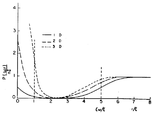
FIG. 32.: Schematic drawing of the local density of states correlation function (normalized by the product $n_{0}^{2}$ of the density of states) as a function of $r=|\vec{r}|$ (in units of $\xi$) for $\omega\ll\Delta$. Taken from Ref. [531].

Analytical progress in understanding level statistics in the localized regime is possible with the help of suitable model systems. Here, we consider the quasi one–dimensional mesoscopic wire with unitary symmetry for which transfer matrix techniques should be useful. (This system is further discussed in the context of transport properties, cf. Sec. VI C). Altland and Fuchs [534] used the results of Ref. [44] and, in the spirit of the transfer matrix approach, reduced the calculation of $R(\omega,L)$ (see Eq. (1)) to the solution of the differential equations

$$\left[-\partial_{t}+{\cal O}\right]Y_{0}(\lambda,t) = 0,\qquad Y_{0}(\lambda,0)=1\ ,$$ (27)

$$\left[-\partial_{t}+{\cal O}\right]Y_{-}(\lambda,t) = Y_{0}(\lambda,t),\qquad Y_{-}(\lambda,0)=0\ .$$ (28)

Here, $\lambda=(\lambda_{1},\lambda_{2})$ are the radial coordinates for the $Q$ matrix in the unitary case, $t=r/\xi$ with $r$ the coordinate along the wire, and ${\cal O}=\Delta_{r}/16+V(\lambda)$ with $\Delta_{r}$ the radial part of the Laplacian on the manifold of $Q$ matrices and $V(\lambda)=-i(\omega/\pi\Delta_{\xi})(\lambda_{1}-\lambda_{2})$ ($\Delta_{\xi}$ is the level spacing in one localization volume). The ratio $\omega/\Delta_{\xi}$ governs the relative importance of the two terms in ${\cal O}$. The correlation function $R(\omega,L)$ can be expressed in terms of the eigenvalues and eigenfunctions of ${\cal O}$ [534]. In general, Eqs. (28) cannot be solved analytically, and one has to calculate these eigenvalues and eigenfunctions on a computer. The main results were as follows. For $t<1$ the WD and the Altshuler–Shklovskii regimes were recovered, albeit with superimposed oscillations on the scale $\Delta$ in the latter. This non–perturbative effect had not been calculated earlier. For $t>1$ a gradual crossover to the Poisson limit ($R(\omega,L)=0$ as $L\to\infty$) was observed, obeying the scaling law $R(\omega,L)\approx(\xi/L)^{d}f(\omega/\Delta_{\xi})$. The function $f(x)$ is proportional to $\ln x$ for very small frequencies ($x\ll 1$) and proportional to $x^{-3/2}$ for larger frequencies ($x>1$). The latter behavior is reminiscent of the Altshuler–Shklovskii regime, see Eq. (9).

We have seen that in the various regimes relevant for disordered mesoscopic systems, a fairly thorough understanding of spectral fluctuations has been attained. The use of WD statistics frequently served as a reference standard which helped to identify and interpret relevant length and energy scales. The greatest challenge is probably still posed by the phenomenon of localization, in particular by the existence of a metal insulator transition to which we turn next.

3 Critical distribution at the metal insulator transition

For $d>2$ (or, in the symplectic symmetry class, for $d\geq 2$) there occurs generically a metal insulator transition (MIT). It is characterized by the existence of a mobility edge $E_{M}$ which separates extended and localized states. With the help of the Anderson model [32] the mobility edge can be investigated as follows. For disorder values $W$ exceeding a certain critical disorder $W_{M}$ all states in the spectrum are localized. For $W<W_{M}$, however, extended states appear in the center of the band. This means that states in the band center are critical for $W=W_{M}$. We address the question: What are the properties of the energy eigenvalue statistics in the vicinity of or, in the thermodynamic limit, at the MIT? We use the index $M$ to label quantities which refer to the mobility edge.

An early argument due to Altshuler et al. [535] suggesting that the MIT might significantly influence the energy eigenvalue statistics used the following interpretation of the result (4) obtained in Ref. [184] for $\omega>E_{C}$. In the time $\hbar/\omega$ an electron propagates over a distance $L_{\omega}=({\cal D}/\omega)^{1/2}$. This distance is smaller than the system size $L=({\cal D}/E_{C})^{1/2}$. Therefore, cubes of size $L_{\omega}$ possess independently fluctuating spectra, and $\langle\delta N^{2}\rangle$ is proportional to the number of such cubes. For $d=3$, this yields

$$\langle\delta N^{2}\rangle\propto\left(\frac{L}{L_{\omega}}\right)^{3}=\left(\frac{\omega}{E_{C}}\right)^{3/2}\ ,$$ (29)

in keeping with Eq. (4). At the MIT, two important effects have to be taken into account. First, we have $E_{C}\approx\Delta$. Therefore, the range of validity of WD statistics is confined to a few levels at most, and the argument leading to Eq. (29) applies practically to all energies. Second, at the MIT the dimensionless conductance $g$ is expected to approach a critical value $g_{M}$ wich is independent of the system size $L$. Imposing this condition, one finds that the diffusion constant ${\cal D}$ becomes scale–dependent, ${\cal D}={\cal D}(L)$ with ${\cal D}(L)\propto 1/L$ for $d=3$. Taking these points into account, Altshuler et al. [535] could estimate the behavior of $\langle\delta N^{2}\rangle$,

$$\frac{\langle\delta N^{2}\rangle}{\langle N(\omega)\rangle}=\chi\approx 0.25\ .$$ (30)

This result was closer to the Poisson distribution (which gives $\langle\delta N^{2}\rangle=\langle N\rangle$) than to Random Matrix Theory (which gives $\langle\delta N^{2}\rangle\approx\ln\langle N\rangle$). The corresponding estimate for the nearest neighbor spacing distribution $P(s)$ with $s=\omega/\Delta$ gave

$$P(s)\propto\exp(-s/\chi)\ ,$$ (31)

which again is reminiscent of the Poisson distribution. It turned out, however, that these arguments were oversimplified and that the estimates (30) and (31) had to be revised.

Shklovskii et al. [536] were the first to formulate the idea that the nearest neighbor spacing distribution $P_{M}(s)$ at the MIT might be universal, thus representing a third possibility besides the Wigner–Dyson statistics $P_{WD}(s)$ and the Poisson law $P_{P}(s)$. In the band center of a three–dimensional Anderson model, and in the thermodynamic limit $L\to\infty$, one expects that $P(s)=P_{WD}(s)$ below the critical disorder ($W<W_{M}$) and $P(s)=P_{P}(s)$ above it ($W>W_{M}$). For $W>W_{M}$, this is because $P(s)$ is the superposition of the contributions from infinitely many and statistically independent localization volumes. For $W<W_{M}$, on the other hand, the range of validity of Wigner–Dyson statistics is extended to infinity since $E_{C}/\Delta$ diverges in the thermodynamic limit. Precisely at the MIT these arguments do not apply since the localization length $\xi(W)$ diverges and $E_{C}\approx\Delta$. This fact led to the postulate [536] of a third “critical” distribution, which was believed to be a hybrid of $P_{WD}(s)$ and $P_{P}(s)$. Linear short–range level repulsion was expected to be followed by Poisson–like behavior, in agreement with Ref. [535].

To check the hypothesis of a third universal distribution, an interesting test was developed and performed in Ref. [536]. We consider the integral $A=\int_{2}^{\infty}P(s)ds$ over the tail of $P(s)$. We recall that $s$ is the energy differenc $\omega$ in units of the level spacing $\Delta$. Moreover, $P_{WD}(s)$ and $P_{P}(s)$ coincide near $s=2$. The quantity

$$\gamma(W,L)=\frac{A-A_{WD}}{A_{P}-A_{WD}}$$ (32)

vanishes for WD statistics, and equals unity for the Poisson distribution. In the thermodynamic limit, $\gamma(W,L)$ exhibits a sharp crossover from $\gamma=0$ to $\gamma=1$ as $W$ crosses the critical value $W_{M}$. (For finite $L$ the crossover is smooth). If a critical, size–independent distribution at the MIT were to exist, the curves of $\gamma(W,L)$ as functions of $W$ and for fixed but different $L$ should all intersect at one critical point $W_{M}$ (in Fig. 33 this point is denoted by $W_{c}$). Furthermore these curves should obey the scaling law

$$\gamma(W,L)=f(L/\xi(W))$$ (33)

with $\xi(W)$ the correlation length of the metal insulator transition. These expectations were numerically verified in Ref. [536], and estimates for both $W_{M}$ and the critical exponent $\nu$ of the localization length were given.

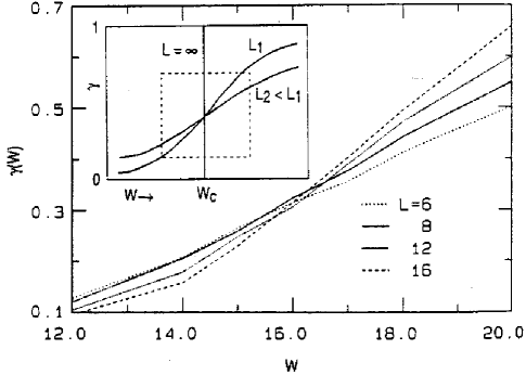
FIG. 33.: The quantity $\gamma(W,L)$ as a function of $W$ for different system sizes $L$ from numerical diagonalization. Inset: schematic figure illustrating the smooth crossover behavior for finite system sizes. Taken from Ref. [536].

Further numerical confirmation for the scenario developed in Ref. [536] was provided by Hofstetter and Schreiber [537]. In particular it was verified that while for $W<W_{M}$ and $W>W_{M}$ the function $P(s)$ tends to the Wigner–Dyson and the Poisson distribution, respectively, as the system size increases, a size–independent third distribution emerges for $W=W_{M}$. This fact and the critical behavior of the quantity $\gamma$ defined in Eq. (32) were exploited in Refs. [538, 539] to determine, as done in Ref. [536], $W_{M}$ and the critical exponent $\nu$ from the spectral statistics alone. The results ($W_{M}=16.5$, $\nu=1.34\pm.10$ [538] and $W_{M}=16.35$, $\nu=1.45\pm.08$ [539]) were consistent with each other and with earlier independent findings [540]. A similar exponent, $\nu=1.35\pm 0.10$, was found by Berkovits and Avishai [541] in a three–dimensional quantum bond percolation system. This suggests that the Anderson and the quantum percolation model are in the same universality class.

Analytical work by Kravtsov et al. [542] led to a first indication that the result (30) was not completely correct. From the analytical derivation of the asymptotic behavior of the two–level correlation function

$$R(s)\propto s^{-2+\gamma}\quad(s\gg 1)$$ (34)

where $\gamma=1-(\nu d)^{-1}$ it was concluded [542] that

$$\langle\delta N^{2}\rangle\propto\langle N\rangle^{\gamma}$$ (35)

instead of Eq. (30). The constants of proportionality in Eqs. (34) and (35) depend only on $d$ and the symmetry class (unitary, orthogonal, or symplectic), thus confirming the universality of the statistics at the MIT. The absence of a term linear in $\langle N\rangle$ was attributed to the sum rule $\int_{-\infty}^{\infty}R(s)ds=0$ [542, 543] (see also Refs. [133, 147]), which together with

$$\frac{d\langle\delta N^{2}\rangle}{d\langle N\rangle}=\int_{-\langle N\rangle}^{\langle N\rangle}R(s)ds$$ (36)

implies that the coefficient of the linear term vanishes for sufficiently large $\langle N\rangle$. With the help of a certain “plasma” model [544], which re–interprets the distribution of levels as the distribution of interacting classical particles in one dimension, cf. Eq. (9), it was possible [543] to deduce the asymptotic form of $P_{M}(s)$,

$$P_{M}(s)\propto\exp(-\tilde{c}s^{2-\gamma})\quad(s\gg 1)\ ,$$ (37)

with $\tilde{c}$ some constant. This was again at variance with previous claims [535, 536] that $P_{M}(s)$ should be Poisson–like. Moreover, numerical work [545] indicated the presence of both a linear term and a term proportional to $\langle N\rangle^{\gamma}$ in the number variance. The situation obviously called for clarification.

Progress was made when the above–mentioned sum rule was critically examined [546, 521]. Although valid (in the limit $\langle N\rangle\to\infty$) for any finite system size, the sum rule may be violated [521] in the thermodynamic limit. In other words, the limits $\langle N\rangle\to\infty$ and $L\to\infty$ do not commute. This insight invalidated the claim that there could be no linear term in $\langle\delta N^{2}\rangle$. The number variance at the critical point was therefore now expected to have the form

$$\langle\delta N^{2}\rangle=A\langle N\rangle+B\langle N\rangle^{\gamma}\ .$$ (38)

But why had earlier investigations [535] missed the non–trivial exponent $\gamma$? Some light was shed on this question by a transparent derivation of the relation (34) by Aronov, Kravtsov and Lerner who combined a semiclassical approach with scaling ideas [547]. We consider the spectral form factor (cf. the closely related quantity $b_{2}(t)$ in Eq. (59))

$$K(t)=\frac{1}{2\pi}\int R(s)\exp(ist)ds\ .$$ (39)

This form factor can be related to the return probability $P(t)$ for a classically diffusing particle [548],

$$K(t)=\frac{2tP(t)}{4\pi^{2}\beta}\ .$$ (40)

This relation is quite powerful. We recall that $t_{d}=\hbar/E_{C}$ is the diffusion time through the system. In the ergodic regime $t\gg t_{d}$ we have $P(t)={\rm const.}$, $K(t)\propto t$ and hence $R(s)\propto 1/s^{2}$, which corresponds to Wigner–Dyson statistics. In the diffusive regime $t<t_{d}$, on the other hand, $P(t)\propto(Dt)^{-d/2}$, $K(t)\propto t^{1-d/2}/{\cal D}^{d/2}$ and Eq. (9), i.e. the result derived by Altshuler and Shklovskii [184], is recovered. As in Ref. [535], the transition from the diffusive to the critical regime was made with the help of the idea that the diffusion constant ${\cal D}$ becomes scale–dependent. Close to the MIT, the dimensionless conductance scales as $g(L)=g_{M}(1+(L/\xi)^{1/\nu})$ with some critical value $g_{M}$ [31]. On the other hand, $g\propto{\cal D}L^{d-2}$ and, therefore,

$${\cal D}(L)\propto g_{M}L^{2-d}\left[1+\left(L/\xi\right)^{1/\nu}\right]\ .$$ (41)

In Ref. [535] the approximation $g(L)\approx g_{M}$ was used, and the square bracket in the relation (41) was absent. This leads to a time–independent spectral form factor and, asymptotically, to $R(s)=0$. Therefore the predictions in Ref. [535] were close to the Poisson case. With the more accurate expression (41) for ${\cal D}(L)$ both time dependence and the non–trivial exponent $\nu$ enter the form factor $K(t)$, and Eq. (34) is recovered [547]. In this way, the controversial issues associated with the two terms in the number variance (38) were resolved.

Several numerical investigations added new aspects to the discussion of the critical level distribution. Evangelou [549] and Varga et al. [550] found that $P_{M}(s)$ can be parametrized accurately by the function

$$P_{M}(s)=c_{1}s\exp\left(-c_{2}s^{2-\gamma}\right)\ ,$$ (42)

with $\gamma=1-(\nu d)^{-1}$ as above and $c_{1}$ and $c_{2}$ two $\gamma$–dependent normalization constants. This was in good agreement with both the expected short–range level repulsion [536] and the asymptotic form (37). (We note, however, that Zharekeshev and Kramer [551] fitted numerical data with $P_{M}(s)\propto\exp(-\tilde{c}s)$, with $\tilde{c}$ some constant, and identified only the linear term in $\langle\delta N^{2}\rangle$). Detailed direct numerical calculations of the spectral two–point function $R(s)$ by Braun and Montambaux [518] provided the probably most complete picture of the behavior of this quantity. In the metallic phase both the random matrix regime and (for the first time) the Altshuler–Shklovskii regime could be identified (cf. Fig. 31). At the mobility edge, the short–range correlations were found to be weakened and the ensuing power–law behavior for larger $s$ was consistent with the picture of anomalous (scale–dependent) diffusion discussed above. Some evidence was found, however, that the linear term in the number variance might have a rather small, or even vanishing, coefficient. In Ref. [552] the asymptotic form (37) and the relation $\gamma=1-(\nu d)^{-1}$ were confirmed for the center of the lowest Landau band in a quantum Hall system.

Does the breaking of time–reversal symmetry affect the critical distribution? This is a controversial issue. While no effect of a magnetic field has been seen by Hofstetter and Schreiber [553], a recent investigation by Batsch et al. [554] reported a universal (i.e. size–independent) crossover behavior from the critical orthogonal distribution discussed so far to a new and distinct critical unitary distribution. A third type of critical distribution was found in two–dimensional systems with spin–orbit scattering [555, 556]. These systems have symplectic symmetry and do exhibit a MIT, in contrast to two–dimensional unitary or orthogonal systems.

Chalker, Lerner, and Smith [557] used a Brownian motion model to describe the energy level statistics at the mobility edge. For the model

$$H(\tau) = H_{0}+\int_{0}^{\tau}d\tau^{\prime}V(\tau^{\prime},\vec{r})\ ,$$ (43)

$$H_{0} = -\frac{\hbar^{2}}{2m}\nabla^{2}+U(\vec{r})\ ,$$ (44)

where both $U(\vec{r})$ and $V(\tau,\vec{r})$ are random white noise potentials, one can derive a Langevin equation governing the parametric dependence of the eigenvalues $E_{n}$ on $\tau$ [557],

$$\frac{dE_{n}(\tau)}{d\tau}=v^{2}\sum_{l\neq 0}\frac{c_{n,n+l}(\tau)}{E_{n}(\tau)-E_{n+l}(\tau)}+\xi_{n}(\tau)\ .$$ (45)

Here, $\xi_{n}(\tau)$ is a random force and the coefficients $c_{nm}(\tau)$, which are given by $c_{nm}(\tau)=L^{d}\int d^{d}r|\psi_{n}(\tau,\vec{r})|^{2}|\psi_{m}(\tau,\vec{r})|^{2}$, contain information on eigenfunction correlations. By solving Eq. (45) approximately, a generalization of the expression (40) for the spectral form factor could be derived, linking spectral statistics with correlations in the wave functions (through the coefficients $c_{nm}$). The two main results derived within this approach were an asymptotic power law for the parametric two–point function $R(s,\lambda\propto\tau^{2})$ at the MIT [557],

$$R(0,\lambda)\propto\lambda^{2/(1+\eta/d)}$$ (46)

and an exact result for the spectral compressibility [558],

$$\frac{d\langle\delta N^{2}\rangle}{d\langle N\rangle}=\frac{\eta}{2d}\quad(\langle N\rangle\gg 1)\ ,$$ (47)

i.e. the coefficient of the linear term in Eq. (38). Here, $\eta=d-d_{2}$, where $d_{2}$ is the multifractal exponent governing the behavior of the inverse participation ratio. These results demonstrate that spectral statistics at the MIT are influenced by the multifractal properties of critical eigenstates.

In spite of considerable progress, the eigenvalue statistics at the mobility edge must, at least in its details, still be considered an open question.

B Persistent currents

An isolated mesoscopic ring threaded by a magnetic flux $\phi$ carries a persistent current $I$ as a thermodynamic equilibrium property. This amazing fact comes about as follows. An electron moving once around the ring picks up a phase factor $\exp(2i\pi\phi/\phi_{0})$ where $\phi_{0}=hc/e$ is the elementary flux quantum. Therefore, all observables depend periodically on $\phi$. This applies, in particular, to the free energy $F=\beta^{-1}\ln{\rm tr}\exp(-\beta H)$, so that $\partial F/\partial\phi$ differs from zero. The equilibrium current $I$ is then given by the thermodynamic relation

$$I=c\frac{\partial F}{\partial\phi}.$$ (48)

The current does not decay in time, hence the name “persistent current”.

Persistent currents have played a central role in mesoscopic physics, for several reasons. First, their existence obviously hinges on the condition that the wave function of the system be coherent over a length scale given by the circumference $L$ of the ring. This must be true even in the case of multiple scattering by impurities. At the beginning of the mesoscopic era, the existence of phase coherence in the diffusive regime was a controversial issue. The positive answer to this question paved the way to experimental and theoretical investigations of a number of interference phenomena. Second, Eq. (48) shows the close connection between the persistent current, the sensitivity of eigenvalues to boundary conditions, and energy level statistics, putting the study of the persistent current at the heart of mesoscopic physics. Third, the problem of persistent currents brought to the fore the important differences between open and isolated (closed) systems. It turned out, in particular, that the grand canonical ensemble commonly used in the calculation of transport properties is inappropriate to describe persistent currents. The grand canonical ensemble has to be replaced by the canonical ensemble, and this caused technical problems. Fourth, experimental values of the persistent current could not be explained in the framework of theories for independent electrons. This was unexpected since theories neglecting the electron–electron interaction had been very successful in modeling transport properties of mesoscopic systems. Seemingly, electron–electron interactions are more important in closed than in open systems. A satisfactory theory with interactions that both reproduces the measured properties of the persistent current and explains why interactions are less critical for open systems is still lacking.

After explaining the early insights and ideas leading to the theoretical prediction of persistent currents, we describe the three experiments performed up to now. In a third part we review analytical calculations neglecting interactions. In this section, aspects of Random Matrix Theory come into play. Therefore, we devote considerable space to this discussion. Finally, we briefly summarize the present status of theories which include the interaction between electrons. A more comprehensive review of the topic can be found in Ref. [559].

1 Early theory, and the three experiments

It has been realized a long time ago [560, 561] that persistent (dissipationless) currents occur in ideal rings free of impurities and interactions. This fact was rediscovered and reformulated more than twenty years later [562, 563]. Expanding on our introductory remarks above, we consider an ideal one–dimensional ring threaded by a magnetic flux $\phi$. The magnetic field can be gauged away from the Hamiltonian [562] at the expense of introducing a twisted boundary condition for the wavefunction, $\psi(x+L)=\exp(2i\pi\phi/\phi_{0})\psi(x)$, where $x$ is the coordinate along the ring. The eigenfunctions at zero field are given by $\exp(2i\pi mx/L)$, and the corresponding eigenvalues are $(\hbar^{2}/2m_{e})(2\pi/L)^{2}m^{2}$, where $m$ is the quantum number of the $z$ component of angular momentum (perpendicular to the plane of the ring). At finite field we have to replace $m$ by $m-\phi/\phi_{0}$. This leads to a quadratic dependence of the single–particle energies on magnetic flux. Equation (48) shows that at zero temperature, the persistent current is given by the sum over all occupied single–particle levels of the flux derivatives of the single–particle energies $E_{m}$,

$$I=-\sum_{m}\frac{\partial E_{m}}{\partial\phi}\ .$$ (49)

This relation explicitly shows the close connection between persistent currents, energy level statistics, and the sensitivity of the spectrum to an external perturbation alluded to above.

Interest in this topic was greatly enhanced by a seminal paper of Büttiker, Imry, and Landauer [564]. These authors claimed that persistent currents exist in normal–metal rings even at finite temperature and in spite of multiple elastic scattering. Their work was followed by a series of papers on 1d [565, 566] and multichannel [567, 568, 569] rings with non–interacting electrons. These investigations tried to assess the chances to actually observe persistent currents in experiments by considering the influence of channel number, temperature and disorder. The main results of these papers can be summarized as follows. In ideal 1d rings with a fixed number $N$ of particles, the persistent current is a sawtooth–shaped function of $\phi$ jumping from $-I_{0}=-ev_{F}/L$ to $+I_{0}$ ($v_{F}$ being the Fermi velocity) at even ($N$ even) or odd ($N$ odd) multiples of $\pm\phi_{0}/2$. The typical current $I_{\rm typ}=\langle I^{2}\rangle^{1/2}$ is given by $I_{0}\sqrt{M}$, i.e. it grows with the number $M$ of channels. The relevant energy scale for temperature effects is the single–particle (rather than the many–particle) level spacing $\Delta$. In the presence of disorder, the Fermi velocity $v_{F}$ in the expression for $I_{0}$ is replaced by the diffusion velocity $L/t_{d}$, and the dependence on the channel number vanishes, $I_{\rm typ}=I_{0}\ell/L$. The average current, on the other hand, was found to decay exponentially with $L$ on the scale of the elastic mean free path $\ell$.

Bouchiat, Montambaux et al. [570] showed that this last assertion is incorrect, for a very fundamental reason. For closed systems in the mesoscopic regime, it is of vital importance to keep the particle number in the system exactly constant as one averages over the disorder configurations. Thus it is necessary to employ the canonical ensemble. The exponentially small currents found in Ref. [568] were shown to be an artifact produced by the use of the grand canonical ensemble, i.e. by keeping the chemical potential (rather than the particle number) fixed in the averaging process. The thermodynamic limit does not apply to mesoscopic rings, and the two ensembles are not equivalent. By a combination of analytical arguments and extensive numerical simulations, the following results for an ensemble of isolated rings were obtained [570]. The typical current $I_{\rm typ}=(\langle I\rangle)^{1/2}$ is independent of channel number $M$ while the average current decreases with increasing disorder and channel number like $\langle I\rangle=I_{0}(\ell/ML)^{1/2}$. Furthermore, the persistent current was found to be periodic in the flux with period $\phi_{0}/2$. This period halving comes about because the ensemble considered contained rings with even and odd particle numbers. The most important result of Ref. [570] was the comparatively large value for the average current. Experimental confirmation of the theoretically predicted phenomenon of persistent currents suddenly seemed to be within reach.

The first experiment on persistent currents was performed by Levy et al. [571] who used an ensemble of $10^{7}$ copper rings mounted on a single wafer. For technical reasons, these rings were actually squares, with a circumference of $L=2.2\mu$m. With $L\gg\ell$, the experiment probed the diffusive regime. A magnetic flux with a small, slowly varying ac component was applied to the sample and the resulting magnetization measured. The ac component allowed for an effective background rejection. The measured current was indeed $\phi_{0}/2$–periodic, in agreement with the numerical simulations [570], see Fig. 34. The average current per ring was $0.4\ nA$, corresponding to $3\times 10^{-3}ev_{F}/L$. This first observation of persistent currents was a striking confirmation of the theoretical ideas developed earlier. However, the current was roughly one order of magnitude larger than the values estimated in Ref. [570].

Two more experiments followed [572, 573]. Both provided interesting additional information that went beyond Ref. [571]. Chandrasekhar et al. [572] investigated three single gold loops. Two of these actually were rings with diameters of $2.4$ $\mu$m and $4.0$ $\mu$m, respectively. The third loop was a rectangle of dimensions $1.4$ $\mu$m $\times 2.6$ $\mu$m. Transport measurements for gold films fabricated like the loops gave an elastic mean free path $\ell=70$ nm. Therefore, all three probes were in the diffusive regime. The observed current was flux–periodic with period $\phi_{0}$. The measured amplitudes at a temperature of $4.5$ mK were in the range $0.2-3.0$ $ev_{F}/L$. The absence of period halving is an immediate consequence of measuring the response of single rings. No averaging over even and odd particle numbers as in the previous experiment was involved. The large amplitudes, however, pose a serious problem. Even when compared with the theoretical estimates for the typical current cited above, these values are larger by one to two orders of magnitude. In comparison with the theoretical average current the discrepancy becomes even worse.

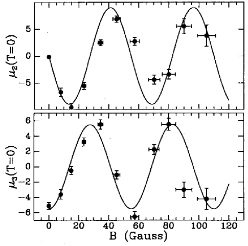
FIG. 34.: The second (top) and third (bottom) zero–temperature harmonic of the magnetic moment (induced by persistent currents in an ensemble of $10^{7}$ copper rings) versus the dc magnetic field. The Fourier decomposition was made with respect to the frequency of a small ac component in the field. One flux quantum through a single ring corresponds to 130 G. The magnitude of the oscillatory moment is estimated to be roughly $10^{-15}$ Am². Taken from Ref. [571].

The third persistent current experiment by Mailly, Chapelier, and Benoit [573] poses less of a problem for theory. In this experiment, the magnetic response of a single mesoscopic GaAlAs/GaAs ring was measured. This ring had an internal diameter of $2$ $\mu$m and an elastic mean free path $\ell=11\mu$m. It was therefore in the ballistic regime. In contrast to the previous two experiments, where the channel number $M$ was of the order of $10^{4}$, $M$ was quite small, $M=4$. A very interesting feature of the semiconductor ring was the possibility to connect it via an electrostatic gate to two external leads. A second gate was placed on one of the arms of the ring, making it possible to suppress all interference effects. With this unprecedented control over the ring it was possible to measure transport and thermodynamic properties in the same system. The current observed in the ring had the value $I_{0}=ev_{F}/L$, exactly as expected for an almost clean sample with very few channels.

In summary, the persistent currents predicted theoretically were observed in three independent experiments. In the diffusive regime, the measured values exceeded theoretical expectations by at least one to two orders of magnitude. This poses a serious challenge for theory.

2 Analytical theory for non–interacting electrons

The need to calculate the disorder average for the persistent current within the canonical (rather than the grand canonical) ensemble [570] led to three almost simultaneous publications by Schmid [574], v. Oppen and Riedel [575], and Altshuler, Gefen, and Imry [576]. The calculations for the average persistent current used the impurity perturbation technique. In Refs. [574, 576], the constraint of constant particle number $N$ was met by letting the chemical potential fluctuate, $\mu=\bar{\mu}+\delta\mu$, and by choosing $\delta\mu$ in such a way that – to first order in $\delta\mu$ – $N$ remained fixed. In Ref. [575], this approximation was avoided by relating the average current to the typical fluctuation of a single level, and by calculating the latter quantity using standard Green function techniques. Strictly speaking, the perturbative results derived in [574, 575, 576] are divergent at zero temperature $T$ and for vanishing flux $\phi$. However, this divergence is regularized either by finite values of $T$, or by the energy scale $1/\tau_{\varphi}$ set by inelastic processes. Both of these scales can realistically be assumed to be at least of the order of the single–particle level spacing $\Delta$. With this assumption, all three investigations yielded for the first even harmonics $I_{m}$ of the persistent current the values

$$I_{m}\approx\frac{\Delta}{\phi_{0}}\approx\frac{ev_{F}}{LM}=\frac{I_{0}}{M},$$ (50)

where $\Delta\approx hv_{F}/LM$. At first sight this seemed to contradict earlier numerical results [570] according to which the average current behaves as $\langle I\rangle\approx I_{0}(\ell/LM)^{1/2}$. However, it was pointed out in Ref. [576] that the first $\sqrt{E_{C}/\Delta}$ harmonics contribute to the current provided the regularizing cutoffs discussed above are of order $\Delta$. (Here, as always, $E_{C}=\hbar{\cal D}/L^{2}$ is the Thouless energy and ${\cal D}$ the diffusion constant). With $E_{C}/\Delta=g=M\ell/L$ and $g$ the dimensionless conductance, these considerations led to a maximal amplitude of

$$I_{\rm max}\approx\frac{\sqrt{\Delta E_{C}}}{\phi_{0}}\approx\frac{ev_{F}}{L}\sqrt{\frac{\ell}{ML}}\ ,$$ (51)

in good agreement with Ref. [570]. Unfortunately, these analytical results did not remove the discrepancy between theory and experiment: As stated above, the result (51) is too small by one to two orders of magnitude.

Altland et al. [577] used Random Matrix Theory and the supersymmetry method to calculate the persistent current non–perturbatively at zero temperature in the model of independent electrons. In this work, a novel approach was used to calculate the impurity–ensemble average within the canonical ensemble. The condition that all rings in the ensemble carried an integer (but not the same) number of electrons was imposed. The resulting expressions turned out to be equivalent to those obtained from the first–order expansion in $\delta\mu$ referred to above. The non–perturbative treatment removed the divergence typical for perturbative results and yielded the current at $T=0$, where all cutoffs lose their physical significance. This work [577] also contained the first calculation of the crossover from orthogonal to unitary symmetry within the supersymmetry formalism. The crossover occurs as the flux increases from $\phi=0$ (where orthogonal symmetry applies) to non–zero values. In keeping with the scope of our review, we discuss this application of Random Matrix Theory in more detail than previous work.

The persistent current $I(\phi)$ can be expressed as follows,

$$I(\phi)=-2\sum_{n=1}^{N}\frac{\partial E_{n}}{\partial\phi}=-2\int_{0}^{E}dE^{\prime}\,\left[\sum_{n=1}^{\infty}\frac{\partial E_{n}}{\partial\phi}\delta(E^{\prime}-E_{n})\right].$$ (52)

The factor 2 accounts for spin degeneracy. To account for the constraint of fixed particle number $N$, the upper integration limit $E$ has to be adjusted as a function both of flux and of disorder realization. This is impossible in practice. The difficulty is avoided as follows. We recall that the first experiment [571] used a wafer with $10^{7}$ rings. It is natural to expect that the particle numbers on these rings, although integer, were different. This suggests averaging $I$ over a range $K$ of particle numbers centered at some value $N_{0}\gg K$. The associated eigenvalues $E_{N}$ defining the upper limit of integration lie in an energy interval $S$,

$$I(\phi)=-\frac{2}{K}\int_{S}dE\int_{0}^{E}dE^{\prime}\,\left[\sum_{n=1}^{\infty}\frac{\partial E_{n}}{\partial\phi}\delta(E^{\prime}-E_{n})\right]\left[\sum_{N=1}^{\infty}\delta(E-E_{N}-\epsilon)\right].$$ (53)

Here, $E_{N}$ is the energy for which there are exactly $N$ electrons on the ring. The second $\delta$ function with infinitesimal positive increment $\epsilon$ in Eq. (53) guarantees the discreteness of the particle number in the ensemble of rings. At first sight nothing has been gained, the problem of adjusting $E$ has just been replaced by the problem of adjusting the full interval $S$. However, as is explained in detail in [577], the dependence of $S$ on flux and disorder can be neglected for $K\gg 1$. Expressing the $\delta$ functions in Eq. (53) in terms of Green functions we get for the ensemble–averaged persistent current

$$\langle I(\phi)\rangle = -\frac{2}{K}\int_{S}dE\int_{0}^{E}dE^{\prime}\,g(E,E^{\prime})$$ (54)

$$g(E,E^{\prime}) = \overline{\frac{1}{4\pi^{2}}{\rm tr}\left[\frac{\partial H}{\partial\phi}\frac{1}{E^{\prime+}-H}\right]{\rm tr}\left[\frac{1}{E^{-}-H}\right]+{\rm c.c.}}\ .$$ (55)

This is equivalent [577] to the expression $\langle I\rangle=\Delta\partial_{\phi}\overline{\left(\int_{0}^{\mu}dE\,{\rm tr}[\delta(E-H)]\right)^{2}}$ employed in Ref. [576] (apart from a sign error in Ref. [576]).

In Ref. [577], the model Hamiltonian (cf. Sec. II C),

$$H(\phi)=\frac{1}{2m}\left(\vec{p}-e\vec{A}\right)^{2}+V(\vec{x})$$ (56)

$$\overline{V(\vec{x})}=0;\quad\overline{V(\vec{x})V(\vec{y})}=\frac{1}{2\pi\nu\tau}\ \delta(\vec{x}-\vec{y})\$$ (57)

was used. Here, $\nu=1/\Delta V$ is the density of states (with $V$ the volume of the ring) and $\tau$ is the elastic scattering time. (Instead of a Gaussian random white noise potential as in Eq. (57), the Hamiltonian could have been chosen as a chain of coupled GOE matrices, see the IWZ model in Sec. VI C 3. Both models lead to the same non–linear $\sigma$ model). Introducing a supersymmetric generating functional for the Green functions as well as for the flux derivatives of $H$, one can write the average current as

$$\langle I(\phi)\rangle=\frac{1}{8\pi^{2}K}\int_{S}dE\int_{0}^{E}dE^{\prime}\,\Bigg{[}\left(\partial_{\phi_{\chi}}-\partial_{\phi_{s}}\right)\partial_{j}\overline{Z[\phi_{s},\phi_{\chi},j]}\bigg{|}_{j=0;\phi_{s}=\phi_{\chi}=\phi}$$ (58)

$$\hskip 227.62204pt+\ {\rm c.c.}\Bigg{]}\ ,$$ (59)

$$Z[\phi_{s},\phi_{\chi},j]=\int d[\Psi]\,\exp\left(\frac{i}{2}\int d^{2}x\,\Psi^{\dagger}(\vec{x})L(D+jI_{2})\Psi(\vec{x})\right)\ .$$ (60)

The definitions of the supersymmetric quantities appearing in Eq. (60) can be found in Ref. [577]. For the present purpose the following explanations hopefully suffice, cf. Sec. III C. The inverse propagator $D$ is basically given by $E-H$ with suitable additional matrix structure to account for (i) the different energy arguments $E,E^{\prime}$ and (ii) the necessary extension to the $8$–dimensional superspace. The quantities $\phi_{s},\phi_{\chi}$ are the flux arguments of those “copies” of $H$ which are associated with the Boson–Boson block and the Fermion–Fermion block, respectively. The matrix $I_{2}$ is diagonal with elements $1$ and $-1$. After the usual steps (averaging, Hubbard–Stratonovich transformation, gradient expansion) we obtain the following non–linear $\sigma$ model,

$$\langle I(\phi)\rangle = -\frac{1}{8\pi^{2}K}\frac{\pi^{2}\nu^{2}{\cal D}\ e}{8L}\int_{S}dE\int_{0}^{E}dE^{\prime}\,\int d[Q]\,{\rm trg}[QI_{2}]\ {\rm trg}[\nabla Q\ [\hat{K},Q]]$$ (62)

$$\quad\quad\times\ \exp\left[\frac{\pi\nu}{8}\int\,{\rm trg}[{\cal D}\ (\nabla Q)^{2}+2\Delta E\ LQ]d^{3}r\right]\ ,$$

where $\hat{K}$ is a suitable source matrix, where $\Delta E=E-E^{\prime}$, and where $\nabla=-i\vec{\partial}+(e\phi/L)[\tau_{3},\cdot]e_{\theta}$ is a covariant derivative with the gradient $\vec{\partial}$ and the tangential unit vector $e_{\theta}$. We note that Eq. (62) is of the form of Eq. (1) except for the redefinition $Q\rightarrow-iQ$. The matrix $\tau_{3}$ = diag $(1,-1)$ introduced at the end of Sec. VI A 1 breaks the symmetry between those parts of the $8\times 8$ supermatrix $Q$ that are connected by the operation of time reversal. As in the case of the spectral fluctuations discussed there, this matrix reflects the necessity to calculate the crossover from orthogonal to unitary symmetry for flux values near $\phi=0$. The divergence in the perturbative approaches discussed above originates from this crossover, more precisely from the “zero mode” in Eq. (62) (i.e. from the contribution with $Q\equiv Q_{0}={\rm const.})$ which cannot be treated adequately in a perturbative framework. Actually, symmetry breaking in this zero mode also poses a technical problem in the context of the supersymmetric formulation. The problem arises from the term ${\rm trg}([\tau_{3}Q_{0}]^{2})$ in the covariant derivative, cf. the exponent in Eq. (62). This problem was overcome by a trick which is a precursor of the parametrization of the $T$ matrix in Eq. (15). Focussing attention on the zero mode, one gets

$$\langle I_{0}(\phi)\rangle=-\frac{1}{8\pi^{3/2}}\frac{\sqrt{E_{C}\Delta}}{\phi_{0}}K(y)$$ (63)

with

$$K(y) = \sqrt{y}\int_{0}^{\infty}dx\,\int d[Q_{0}]\,\exp\left(y\ {\rm trg}\ [Q_{0}\tau_{3}Q_{0}\tau_{3}]+\frac{x}{4}\ {\rm trg}\ [Q_{0}L]\right)$$ (65)

$$\quad\quad{\rm trg}\ [Q_{0}I_{2}]\left({\rm trg}\ [Q_{0}\tau_{3}Q_{0}\hat{K}]-4\right)+{\rm c.c.}\ ,$$

where $y=\pi(E_{C}/\Delta)\ (\phi/\phi_{0})^{2}$ and $x=\pi\ \Delta E/\Delta$. After the final integration over $Q_{0}$ the result can be well parametrized by the expression $\langle I\rangle=(\sqrt{E_{C}\Delta}/\phi_{0})\ (\kappa_{1}\sqrt{y}/(1+\kappa_{2}y))$ with $\kappa_{1}\approx 2.25$ and $\kappa_{2}\approx 12.40$. This gives a maximal amplitude of $I_{\rm max}\approx 0.3\sqrt{E_{C}\Delta}/\phi_{0}$, in agreement with the estimates given in Ref. [576]. The modes with spatially varying $Q$ fields can be treated perturbatively and added to the zero mode result to obtain a full picture of the current [577].

In a closely related study, Efetov and Iida [578] calculated the persistent current from a dynamic response. This point of view has the advantage that the dynamic response is not sensitive to the use of the canonical or the grand canonical ensemble. Within the model (57) of non–interacting electrons in a ring threaded by a magnetic flux and with a slowly varying field

$$B(t)=B_{0}+B_{\omega}\cos(\omega t),$$ (66)

the density of the oscillating current can be written in linear response as

$$j_{\omega}=K(\omega)A_{\omega}\ .$$ (67)

Here, $K(\omega)$ is the current–current correlation function and $A_{\omega}$ is the vector potential corresponding to the magnetic field $B_{\omega}$. At first sight it is plausible that the current calculated from Eq. (67) in the limit of vanishing frequency $\omega\to 0$ should be basically equivalent to the thermodynamic current (see, however, the discussion below). The quantity $K(\omega)$ is essentially given by the correlator

$$\tilde{R}(\omega)=\overline{p_{r}G_{E}^{+}(r,r^{\prime})p_{r^{\prime}}G_{E-\omega}^{-}(r^{\prime},r)}\ ,$$ (68)

where $p_{r}=(1/m)[-i\nabla+eA]$ is the velocity operator and $G_{E}^{\pm}$ the retarded (advanced) Green function. This correlator can be expressed in the framework of the supersymmetry method as a functional average $\langle\ldots\rangle_{Q}$ over a field of $Q$ matrices [578],

$$\langle\ldots\rangle_{Q}=\int(\ldots)\exp\left(-S[Q]\right)DQ$$ (69)

with

$$S[Q]=-\frac{\pi\nu}{8}\int{\rm trg}\left(D[\nabla Q-ieA[Q,\tau_{3}]]^{2}+2i\omega LQ\right)dr\ .$$ (70)

This is, of course, absolutely analogous to Eq. (62). Without specifying the precise form of the terms in the angular brackets in Eq. (69) we confine ourselves to saying that the procedure is analogous to the one explained above in the context of the thermodynamic approach. Again, the calculation may be restricted to the zero mode, i.e. to a spatially constant $Q$ field. The final result for the current has a maximal amplitude of the order of $\sqrt{E_{C}\Delta}/\phi_{0}$, in agreement with Ref. [577]. However, the shape of the current as a function of the magnetic flux differs considerably from the one found in the thermodynamic calculation.

The relation between the thermodynamic and the dynamic approaches was addressed by Kamenev and Gefen [579]. These authors investigated a whole variety of averaging procedures, differing (i) in the initial preparation of the system under study and (ii) in the constraints imposed while the external field is varied adiabatically. According to Ref. [579], the thermodynamic calculation corresponds to the situation where both the initial occupation of levels and the evolution of the system with varying flux are determined within the canonical ensemble. The dynamic response, on the other hand, corresponds to a particular procedure: The initial occupation of levels is defined grand–canonically but is then held fixed as determined by the canonical ensemble. Hence there is no reason why the persistent currents calculated in both cases should coincide exactly. On physical grounds, however, one does not expect drastic (order–of–magnitude) discrepancies.

The same authors also investigated the magnetoconductance [580] and the conductance distribution [581] of isolated rings in the quantum regime, where the level widths are smaller than the level spacing. Significant differences between the canonical and the grand canonical ensemble were found.

3 Theories with electron–electron interaction

After it had generally been recognized that the experimental values for the persistent current could not be explained in the framework of theories which neglect the electron–electron interaction, numerous investigations appeared which addressed the role of these interactions. A detailed discussion of this vast body of work is completely beyond the scope of the present review which focusses on Random Matrix Theory. We restrict ourselves to a brief enumeration of relevant work. The difficulty in attempts to treat both disorder and interaction lies in the fact that disorder alone poses severe theoretical problems (witness the present section) while interactions add the full complexity of the non–relativistic many–body problem.

In an early paper by Ambegaokar and Eckern [582] (actually preceding the full solution of the non–interacting problem [574, 575, 576, 577]), the grand potential of a mesoscopic normal metal ring including electron–electron interactions was calculated to first order in the interaction. Evaluating both the Hartree and Fock diagrams, the authors found that the average persistent current is parametrically given by $E_{C}/\phi_{0}$, in apparent agreement with Ref. [571]. The same result was later derived in Ref. [574] from the condition of local charge neutrality. Also, the temperature dependence of the result, see Ref. [583], was closer to experiment than obtained in theories without interactions. However, diagrams of higher order in the interaction renormalize the Cooper channel and were estimated to reduce the result to roughly one order of magnitude below measured values [584]. A calculation of the typical current along similar lines [585] resulted in a very large value, $I_{\rm typ}\approx ev_{F}/L$, but was later corrected [586] to $I_{\rm typ}\approx ev_{F}\ell/L^{2}=E_{C}/\phi_{0}$. Work using density functional theory [587] also led to relatively large currents of order $E_{C}/\phi_{0}$, but the absence of renormalizing, higher–order corrections could again not be established. Recently, the results of Ref. [582] could be reproduced within a simple (non–diagrammatic) Hartree–Fock picture [588].

In a series of papers, the persistent current problem was approached from the point of view of Luttinger liquid theory. From very early work [589] it was known that in a Luttinger liquid the effect of a single impurity is exponentially enhanced (suppressed) for repulsive (attractive) interactions. It was possible to generalize the formalism to include the case of twisted boundary conditions necessary to describe a clean mesoscopic ring in a magnetic field [590] (see also Ref. [591]). Nevertheless the Luttinger liquid, predicting enhanced impurity scattering for interacting electrons, did not seem to be a promising candidate for explaining the discrepancy between theory and experiment. Interacting Fermions in clean, one–dimensional rings were also investigated in Ref. [592] by means of the Bethe ansatz. In a refined treatment [593] of the effect of impurities which improved on the work of Ref. [589] by going beyond simple perturbation theory for the disorder, spinless Fermions in one dimension and with repulsive interaction were investigated. An algebraic (rather than exponential) decay of the current with the ring circumference was found. On the other hand, Monte–Carlo simulations [594] indicated that for a strong impurity potential, the current may be enhanced. A significant new aspect was contributed to the discussion by Giamarchi and Shastry [595], who took into account the spin degree of freedom. In earlier work [596] on the localization properties of one–dimensional disordered electron systems a combination of the replica trick (to average over disorder) and renormalization group methods was used. The renormalization group equations derived in Ref. [596] were employed in Ref. [595] to prove that repulsive interactions can enhance the persistent current, provided the carriers have spin (see Ref. [597], and also Refs. [598, 599]). This work emphasized the important role of the additional spin degree of freedom and (indirectly) gave rise to the interesting question whether a second channel (i.e., a model beyond the strictly one–dimensional Luttinger liquid) would play a similar role. It was pointed out in Ref. [600] that the enhancement just mentioned does not lead back to the value for the clean ring.

Another approach [601] invoked the classical electromagnetic energy associated with charge fluctuations and long–range Coulomb forces to derive a very large average current of the order of $ev_{F}/L$. The critique [602] leveled against this work basically points out that the assumed coexistence of large fluctuations and long–range forces is highly implausible.

A new mechanism explaining why the Coulomb interaction might indeed counteract the influence of the disorder potential was suggested and investigated in Ref. [603]. The key point was a phase–space argument: By mixing many–particle states in a rather large energy interval, the Coulomb interaction redistributes the strength of the impurity potential to high–lying configurations, thus reducing the influence of impurity scattering on the ground state relevant for the persistent current. Numerical simulations supported this claim, but the relation of the model used to real physical systems remained controversial.

Much important work used computer simulations of lattice models of interacting particles. Small one–dimensional systems of spinless Fermions could be treated by numerical diagonalization of the Hamiltonian, but no enhancement of the persistent current was found [604, 605, 606, 607]. In Ref. [604] this fact was (at least partly) attributed to the onset of the Mott–Hubbard transition which sets in as the interaction strength increases. These results were confirmed in Ref. [608] in the framework of a Hartree–Fock approach. Similar conclusions were also reached in a recent study using the density–matrix renormalization–group algorithm [609]. Numerical investigations of one– and three–dimensional rings [610] which included first–order corrections due to interactions, found (among other results) agreement with Ref. [582] in the diffusive regime.

Exact diagonalization is possible only when the system sizes are severely restricted. It is an important task to devise reliable numerical approximation schemes capable of dealing simultaneously with interactions and disorder. One step in this direction was the development of the self–consistent Hartree–Fock method (SHF) [611, 612]. Through a self–consistency condition, higher–order terms in the interaction are effectively resummed. Therefore, the method goes beyond the analytical calculations in Ref. [582]. With this method, an enhancement of the persistent current has been found in three–dimensional rings and for long–range interactions [612]. A similar enhancement was observed after exact diagonalization of small two–dimensional cylinders with long–range interactions in Ref. [613]. For short–range (on–site and nearest–neighbor) interactions in two dimensions, on the other hand, spin again seems to be an important factor [614]: the current was found to be strongly suppressed in the spinless case but to be significantly enhanced once spin was included.

Why do interactions affect the persistent current but not the conductance? This very important question was addressed by Berkovits and Avishai [615]. The authors expressed the conductance as the compressibility of the system times the flux derivative of the ensemble–averaged persistent current. This formula leads to the plausible scenario that an enhancement of the persistent current is compensated by a corresponding reduction of the compressibilty, with zero net effect on the conductance.

C Transport in quasi one–dimensional wires

The main experimental information on mesoscopic systems is derived from transport studies: Each such system is connected to voltmeters and/or external voltage differences by a number of leads, and both the resistance tensor and, by implication, the conductance tensor are measured. Historically, these experiments raised questions of a conceptual nature. What is the meaning of a transport coefficient like the conductance in a system where inelastic effects and, hence, energy dissipation are absent by definition? This is not the place to review the heated discussion of nearly a decade ago. An overview over this subject is given in an article by Stone and Szafer [616]. Suffice it to say that there are two approaches to quantum transport in mesoscopic systems, the Kubo formula [617] based on linear response theory, and the scattering approach pioneered by Landauer [618], see Eqs. (72) and (74) below. The problem of dissipation in mesoscopic transport was mainly discussed in the framework of Landauer’s ideas. The key issue here were the so–called reservoirs, fictitious sources and sinks for electrons. These reservoirs were introduced to represent the macroscopic contacts attached to the mesoscopic probe. Energy dissipation occurs in, and irreversibility is caused by, these reservoirs. In this way, the conductance of a mesoscopic system could be meaningfully defined even though neither dissipation nor any irreversible processes occur in that system itself. This result can be seen as another manifestation of quantum coherence in mesoscopic systems: The wave function is coherent in the entire domain connecting the reservoirs.

The study of electron transport in quasi one–dimensional (1d) wires is particularly interesting, for several reasons. In contrast to strictly 1d systems, these wires possess a genuine diffusive regime. At the same time, they share many properties with strictly 1d systems. This is true, in particular, for the applicability of non–perturbative analytical methods. In the last decade, both the DMPK equation [619, 620] and the non–linear $\sigma$ model [44, 140] have been successfully used to describe such wires. This has led to an (almost) complete understanding of the physical properties of these wires for all length scales $L$.

By definition, the transverse dimensions of quasi 1d wires are large enough to accomodate a number ($\Lambda$) of transverse quantized modes (often referred to as channels) below the Fermi energy. Typically, $\Lambda$ is of the order $10^{2}$ or $10^{3}$, hence $\Lambda\gg 1$. At the same time, the transverse dimensions are small enough (i.e., of the order of the elastic mean free path $\ell$) so that no diffusion takes place in the transverse direction. The ballistic regime $L<\ell$ and the localized regime $L>\xi$ (with $\xi=\Lambda\ell$) are separated by the diffusive regime $\ell<L<\xi$ where Ohm’s law applies.

In a first part we briefly discuss the phenomenon of universal conductance fluctuations. This phenomenon triggered most of the interest in mesoscopic physics and quasi 1d systems. Subsequently, we describe the two non–perturbative approaches mentioned above. Both originate from or are at least intimately related to the concept of Random Matrix Theory. Lastly, we review the development leading to the insight that these two approaches, in spite of their considerable technical dissimilarity, are in fact equivalent.

1 Universal conductance fluctuations

In 1984, peculiar fluctuations in the conductance of small metallic wires [621, 622] and of small metallic rings [623, 624, 625, 626] were observed experimentally, see Fig. 7. These fluctuations occurred as a function of an external magnetic field. The same phenomenon was found in quasi 1d MOSFETs [627, 628, 629, 630] as a function of gate voltage. The phenomena are reviewed in Refs. [8, 631]. The fluctuations occurred at Kelvin temperatures in systems that were much larger than the elastic mean free path $\ell$, but smaller than the phase coherence length $L_{\phi}$, i.e. in what became known as the mesoscopic regime. Most strikingly, the amplitude of the fluctuations at low $T$ was of the order of $e^{2}/h$, independent of the mean conductance of the sample and of sample–specific details like length, material or geometric shape. Therefore, these fluctuations were dubbed “universal conductance fluctuations” (UCF). The fluctuation pattern turned out to be typical for a given sample and reproducible in consecutive measurements at fixed temperature, hence the name “magnetofingerprints”. This observation ruled out any explanation in terms of time–dependent fluctuation processes. In rings like the one shown in Fig. 30, a superposition of UCF and periodic oscillations of principal frequency $h/e$ was observed, see Fig. 35. This was a demonstration of the mesoscopic Aharonov–Bohm effect [8].

UCF can be qualitatively explained by estimating the level number fluctuations, see Sec. VI A 1, but compared with expectations based on classical physics, the UCF are abnormally large: From Ohm’s law and in $d$ dimensions, we have $\langle g\rangle\propto L^{d-2}$ for the dimensionless mean conductance $\langle g\rangle$. UCF implies ${\rm var}(g)\approx{\rm constant}$. Therefore, the relative fluctuations ${\rm var}(g)/\langle g\rangle^{2}$ of the conductance behave as $L^{2(2-d)}$. For a network of classical resistors of size $L$ in $d$ dimensions, on the other hand, one can show [632] that the relative fluctuations ${\rm var}(g)/\langle g\rangle^{2}$ of the conductance behave as $L^{-d}$: The relative fluctuations vanish as the system size goes to infinity. This is referred to as “self–averaging”. The existence of UCF implies that there is no self–averaging for $d=1,2$.

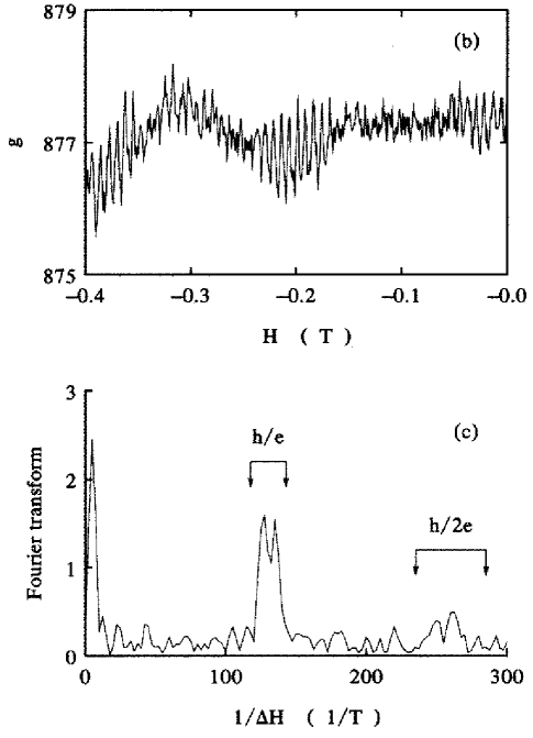
FIG. 35.: Top: The dimensionless conductance $g$ (i.e. the conductance in units of $e^{2}/h$) of a mesoscopic gold loop versus magnetic field. Bottom: The Fourier transform of the data in the top figure. Peaks in the spectral weight are abserved near $1/\Delta H=0$ (UCF), $130/T$ (principal Aharonov–Bohm periodicity), and $260/T$ (higher harmonic). Taken from Ref. [516].

Theoretical investigations by Altshuler, Lee, and Stone revealed that these fluctuations were due to complex quantum interference effects [633] typical for the diffusive regime. The amplitude was indeed found to be universal and of order $e^{2}/h$ [634, 635, 636]. Shortly thereafter, Imry [637] further elucidated the origin of UCF by assuming that the long–range stiffness in the spectra of Gaussian Random Matrix Theory carries over to certain parameters $x_{j}$ characterizing the transfer matrix of a disordered segment. With this assumption the universality of the conductance fluctuations followed immediately. While the assumption was not quantitatively correct, it helped to develop a simple and intuitive understanding of UCF (cf. the discussion of Ref. [184] at the beginning of Sec. VI A 1). We mention that UCF have much in common with but are different from Ericson fluctuations, cf. Sec. IV A.

The analytical modeling used an ensemble of impurity potentials of the kind described in Sec. II C. A general problem of stochastic modeling (first encountered in RMT in the context of nuclear physics, see Sec. II A) resurfaced in the present context: To compare ensemble averages with data, an ergodic hypothesis had to be invoked. It states that an ensemble average over the impurity potential is equal to the running average (taken over a range of values of the magnetic field strength or of the gate voltage) on a fixed member of the ensemble (i.e., the physical sample). This assumption is discussed in some detail in the comprehensive paper by Lee, Stone, and Fukuyama [632].

For a quantitative analysis, the multichannel Landauer formula has been the most useful starting point. This formula has acquired considerable importance in the interpretation of transport properties of mesoscopic systems. It expresses the dimensionless conductance $g$ in terms of the quantum–mechanical transmission amplitudes through the mesoscopic device.

To derive this formula from linear response theory, i.e., from the Kubo formula [617], we consider a finite quasi 1d disordered region in $d$ dimensions with volume $V=L_{\perp}^{d-1}L$. Infinite ideal leads with identical cross sections $L_{\perp}^{d-1}$ are attached to both ends of this rod of length $L$. In this model geometry, the zero temperature Kubo formula for the conductance reads

$$g=\left(\frac{2\pi}{L}\right)^{2}\sum_{k,l}\left|\int_{V}d^{3}r\frac{1}{2im}\left(\nabla\psi_{k}^{*}\psi_{l}-\psi_{k}^{*}\nabla\psi_{l}\right)\right|^{2}\delta(E_{F}-E_{k})\delta(E_{F}-E_{l})\ .$$ (71)

(72)

Here, $E_{F}$ is the Fermi energy, $\psi_{k}$ are the eigenstates of the system (including the leads) and $E_{k}$ the corresponding eigenvalues. The integral extends over the disordered region, and the derivatives are to be taken in the longitudinal direction of the quasi 1d rod. Lee and Fisher [638] have shown that Eq. (72) is equivalent to

$$g = \phantom{2}\sum_{a,b}(|S_{ab}^{RL}|^{2}+|S_{ab}^{LR}|^{2})$$ (73)

$$= 2\sum_{a,b}|S_{ab}^{RL}|^{2}\ ,$$ (74)

where $S_{ab}^{RL}$ and $S_{ab}^{LR}$ are those elements of the scattering matrix that connect the right lead ($R$) with the left one ($L$) and vice versa, respectively. Eq. (74) is known as the multichannel Landauer formula [639, 638]. It establishes a direct link between the conductance and scattering theory, and has been extended to the case of many external leads by Büttiker [640]. The proof of equivalence of the Kubo and the Landauer approach was further generalized by Stone and Szafer [616] and by Baranger and Stone [641]. (In the first of these papers, there are some misleading statements about the lack of unitarity of the scattering matrix which are due to an incorrect normalization of the wave functions).

At first sight, Eq. (74) seems absolutely obvious: Aside from a factor 2 for spin, $g$ is given by the total quantum–mechanical transmission probability through the mesoscopic device. At second sight, one begins to wonder, however: $g$ is expressed in terms of the scattering matrix. This quantity describes the dissipationless passage of electrons through the sample. How is it possible, then, that $g$ is a transport coefficient which accounts for dissipation? This is the issue discussed at the beginning of this subsection. Here, we only emphasize that Eq. (74) is another manifestation of quantum coherence in mesoscopic devices. Because of this coherence, it is problematic to define a conductivity, which would require local dissipation in the probe. Rather, properties of the entire device enter into the definition of the conductance.

The actual calculations employed impurity perturbation theory. An early overview is given in Ref. [632]. This technique is tailored towards the calculation of (products of) Green functions, and the conductance must first be expressed in terms of such functions. This can be done either by expressing the $S$ matrices in Eq. (74) in terms of such functions [140], or by using in Eq. (72) the identity

$$\langle r|G^{+}(E)-G^{-}(E)|r^{\prime}\rangle=-2\pi i\sum_{k}\psi^{*}_{k}(r)\psi_{k}(r^{\prime})\delta(E-E_{k})\ ,$$ (75)

where $G^{\pm}(E)=(E^{\pm}-H)^{-1}$. The resulting expression for $g$ is bilinear in the Green functions. After averaging over the ensemble, the only non–vanishing contribution has the form $\overline{G^{+}(r,r^{\prime};E_{F})G^{-}(r,r^{\prime};E_{F})}$. In essence, the calculation of such a term uses an expansion of the Green functions in powers of the impurity potential $V(r)$. (For the definition of $V(r)$, cf. Eq. 14). The ensuing perturbation series is well defined in the diffusive regime and can be reordered to yield a systematic expansion in powers of the disorder parameter $(k_{F}\ell)^{-1}$. To leading order in $(k_{F}\ell)^{-1}$, the Fourier representation of a single averaged Green function is given by [642]

$$G^{+}(p,p^{\prime})=\frac{\delta(p-p^{\prime})}{E_{F}-p^{2}/2m+i/2\tau}\ .$$ (76)

The average Green function acquires a finite lifetime $\tau=\ell/v_{F}$ (the elastic mean free time). In coordinate space, the Green function decays on the scale of the elastic mean free path. Again to leading order in $(k_{F}\ell)^{-1}$ one can show [642] that the expression $\overline{G^{+}(r,r^{\prime};E_{F})G^{-}(r,r^{\prime};E_{F})}$ is given by the diffusion propagator $\Pi(r,r^{\prime})$, a solution of the equation

$$\tau{\cal D}\Delta\Pi(r,r^{\prime})=\delta(r-r^{\prime}).$$ (77)

Here, ${\cal D}=v_{F}^{2}\tau/3$ is the diffusion constant. Calculating higher moments of the conductance amounts to calculating averages of higher products of Green functions and becomes increasingly complicated. For the variance of the conductance it turns out [634, 635] that

$${\rm var}(g)\propto\int d^{3}r\int d^{3}r^{\prime}\,\Pi(r,r^{\prime})\Pi(r^{\prime},r)={\rm tr}\,\Pi^{2}\ .$$ (78)

For a quasi 1d wire without spin–orbit scattering and obeying time–reversal symmetry, Eq. (78) yields the universal result $8/15$ [635]. For all three symmetry classes with $\beta=1,2,4$, the result is ${\rm var}(g)=8/(15\beta)$.

The impurity perturbation technique sketched above cannot give a complete picture of the transport properties of quasi 1d systems because it fails (as does any perturbative approach) in the localized regime. It is therefore necessary to consider alternative, non–perturbative approaches. This is the program for the remainder of this section on quasi 1d transport.

2 Dorokhov–Mello–Pereyra–Kumar equation

A first non–perturbative approach deals directly with the transfer matrix $M$ of a disordered conductor. This matrix is defined as follows. We consider a disordered sample connected to two ideal leads. The number of channels in each lead is denoted by $\Lambda$. The matrix $M$ expresses the $\Lambda$–dimensional vectors $\phi^{\prime}_{\rm in}$ and $\phi^{\prime}_{\rm out}$ in one lead (which describe the incoming and outgoing wave amplitudes in that lead) in terms of the corresponding $\Lambda$–dimensional vectors ($\phi_{\rm in}$ and $\phi_{\rm out}$) in the other lead,

$$\left[\begin{array}[]{c}\phi^{\prime}_{\rm out}\\ \phi^{\prime}_{\rm in}\end{array}\right]=M\left[\begin{array}[]{c}\phi_{\rm in}\\ \phi_{\rm out}\par\end{array}\right]\ .$$ (79)

The matrix $M$ differs from the scattering matrix $S$. The latter connects the outgoing wave amplituds in either lead with the incoming ones,

$$\left[\begin{array}[]{c}\phi_{\rm out}\\ \phi^{\prime}_{\rm out}\end{array}\right]=S\left[\begin{array}[]{c}\phi_{\rm in}\\ \phi^{\prime}_{\rm in}\end{array}\right]\ .$$ (80)

The two matrices $M$ and $S$ are, of course, not independent but are connected by a non–linear equation not given here. Both matrices yield equivalent descriptions of the scattering process. The virtue and usefulness of the transfer matrix lies in a multiplicative composition rule: The transfer matrix of a number of disordered regions arranged in series and pairwise connected by ideal leads, is the product of the transfer matrices of the individual regions. This property is used in the construction of the transfer matrix in the local approach described below. It relates directly to the scaling theory of localization.

Combining Eqs. (79) and (80) with the Landauer formula (74) one can show that the conductance is given in terms of the radial “eigenparameters” $\lambda_{i}$ (to be defined below) of $M$ as

$$g=2\sum_{i=1}^{\Lambda}\frac{1}{1+\lambda_{i}}\equiv 2\sum_{i=1}^{\Lambda}T_{i}\ ,$$ (81)

where we have defined the transmission eigenvalues $T_{i}=1/(1+\lambda_{i})$. The task is then to determine $M$ and, thus, $\langle g\rangle$ or higher moments of $g$.

Every microscopic realization of a disordered quasi 1d wire is associated with a particular transfer matrix $M$. This fact suggests the basic idea of the transfer matrix approach: To define an appropriate ensemble of transfer matrices that correctly reflects the transport properties of an ensemble of disordered wires. There are two different ways to do so, the global and the local approach. In the global approach developed by Pichard, Stone et al. [643, 644, 645], the statistical properties of the full transfer matrix are determined in a single step: The maximum entropy approach is used in conjunction with physically motivated constraints to determine an ensemble of transfer matrices. In the local approach by Dorokhov [619], Mello, Pereyra, and Kumar [620], the maximum entropy approach is employed to define an ensemble of transfer matrices for a small (but still macroscopic) piece of wire. The decomposition of the wire associated with this model is similar to the one employed in Sec. VI C 3 for the IWZ model, see Fig. 36. The full ensemble of transfer matrices for the entire system is then obtained by putting many of these small pieces in series, i.e. by multiplying the corresponding transfer matrices. This procedure defines a Brownian motion model for the transfer matrix and leads to a Fokker–Planck equation for its “eigenparameters” $\lambda_{i}$. This is the Dorokhov–Mello–Pereyra–Kumar (DMPK) equation. In the following we focus attention on this latter theory. The global approach has been reviewed in detail in Ref. [646].

We briefly sketch the derivation of the DMPK equation. We follow a formulation in Ref. [647] which was applied by Frahm and Pichard [448, 648] in a slightly different context, namely for a Brownian motion model for the $S$ matrix. We restrict ourselves to the case of unitary symmetry ($\beta=2$). The relevant symmetry of $M$ is dictated by current conservation and reads [646]

$$M^{\dagger}\Sigma_{z}M=\Sigma_{z},$$ (82)

where $\Sigma_{z}=$diag$(1,-1)$ in the block representation defined by Eq. (79). Putting $M=\exp(X)$ this implies

$$X=\left[\begin{array}[]{cc}a&b\\ b^{\dagger}&d\\ \end{array}\right]\ ^{\prime}$$ (83)

with $a^{\dagger}=-a$ and $d^{\dagger}=-d$.

Using this symmetry, we now consider $M(x)$ as a function of a variable $x$ which describes the length of the wire. We wish to find a differential equation for $M(x)$. We define a random process by

$$M(x+\delta x)=e^{\delta M}M(x)$$ (84)

where $\delta M$ is a random matrix which must have the same symmetry as $X$. For simplicity, we identify $\delta M$ with $X$ and introduce the following statistical assumptions (which can be justified in terms of a maximum entropy approach [620]): $\delta M$ has a Gaussian probability distribution with vanishing first moment and uncorrelated matrix elements $a,b,d$. The second moments are given by

$$\overline{{\rm tr}(a^{\dagger}a)}=\overline{{\rm tr}(d^{\dagger}d)} = W_{f}\Lambda^{2}\delta x\ ,$$ (85)

$$\overline{{\rm tr}(b^{\dagger}b)} = W_{b}\Lambda^{2}\delta x.$$ (86)

We recall that $\Lambda$ is the number of channels. The quantities $W_{f}$ and $W_{b}$ define the relative strength of the diagonal and non–diagonal elements, respectively.

It is useful to decompose the transfer matrix into radial and angular degrees of freedom,

$$M(x)=Ue^{H}V\ ,\quad M(x+\delta x)=\tilde{U}e^{H+\delta H}\tilde{V},$$ (87)

where $U={\rm diag}(u_{1},u_{2})$, $V={\rm diag}(v_{1},v_{2})$, and $H=\nu\Sigma_{x}$ (and similarly for $\tilde{U},\tilde{V}$, and $\delta H$). Here $u_{i}$ and $v_{i}$ are unitary matrices, $\nu$ is a diagonal matrix of “radial” parameters, and $\Sigma_{x}$ is the first Pauli matrix. The quantities $\nu_{i}$ are related to the “eigenparameters” $\lambda_{i}$ in Eq. (81) through $\lambda_{i}=\sinh^{2}(\nu_{i})$. It is the aim to express the variation $\delta H$ in the radial paramters as a function of the statistical input (86) for the random process (84). This is achieved by an expansion to second order in the small quantities $b$ and $b^{\dagger}$. The quantities of central interest are the increments $\delta\nu_{i}$ of the radial parameters. Their detailed properties follow from Eq. (86). For $\beta=2$ the result reads

$$\overline{\delta\nu_{j}} = \frac{1}{2}W_{b}\delta x\left(\sum_{k(\neq j)}\left(\coth(\nu_{j}-\nu_{k})+\coth(\nu_{j}+\nu_{k})\right)+2\coth(2\nu_{j})\right)\ ,$$ (88)

$$\overline{\delta\nu_{j}\delta\nu_{k}} = \frac{1}{2}W_{b}\delta x\delta_{jk}\ .$$ (89)

This defines a standard Brownian motion process leading immediately [126] to a Fokker–Planck equation for the distribution function $p(\nu,x)$ of the radial parameters (DMPK equation)

$$\partial_{x}p(\nu,x) = \frac{W_{b}}{4}\sum_{j}\partial_{\nu_{j}}\Bigg{(}\partial_{\nu_{j}}-2\sum_{k(\neq j)}\left(\coth(\nu_{j}-\nu_{k})+\coth(\nu_{j}+\nu_{k})\right)$$ (91)

$$\hskip 170.71652pt-2\coth(2\nu_{j})\Bigg{)}p(\nu,x)\ .$$

The differential operator on the r.h.s. of Eq. (91) is the radial part of the Laplacian on the space of transfer matrices [649]. Introducing as new variables the “eigenparameters” $\lambda_{i}=\sinh^{2}(\nu_{i})$, we get an alternative form of the DMPK equation,

$$\partial_{x}\hat{p}(\lambda,x)=\frac{2}{\xi}\sum_{j}\partial_{\lambda_{j}}J(\lambda)\lambda_{j}(1+\lambda_{j})\partial_{\lambda_{j}}J^{-1}(\lambda)\hat{p}(\lambda,x).$$ (92)

With $J(\lambda)=\prod_{j<k}|\lambda_{j}-\lambda_{k}|^{\beta}$, the definition for the elastic mean free path $\ell=1/(W_{b}(\Lambda+(2-\beta)/\beta))$ and the localization length $\xi=\ell(\beta\Lambda+2-\beta)$, Eq. (92) is valid for all three symmetry classes.

The DMPK equation has been solved by Beenakker and Rejaei [650, 651] in the unitary case ($\beta=2$). It is obviously of considerable interest to have an exact solution for the distribution function $\hat{p}(\lambda,x)$. The actual motivation for this work had another source, however: A puzzling discrepancy between the global approach [643, 644, 645] and diagrammatic perturbation theory. In the global approach it is assumed that all correlations among the eigenvalues $\lambda_{i}$ stem from the Jacobian $J(\lambda)$ introduced above. (Formally, this is just the square of the Vandermonde determinant discussed in Sec. III A 2). Therefore the distribution function must have the form

$$\hat{p}_{\rm glob}=e^{-\beta(\sum_{i<j}u(\lambda_{i},\lambda_{j})+\sum_{i}V(\lambda_{i}))}$$ (93)

with the logarithmic two–body repulsion $u(\lambda_{i},\lambda_{j})=-\ln|\lambda_{i}-\lambda_{j}|$ coming from the Jacobian. It was shown by Beenakker [652], however, that Eq. (93) leads to ${\rm var}(g)=1/2\beta$ (instead of the correct value $8/15\beta$), irrespective of the form of the confining potential $V(\lambda_{i})$. Hence the logarithmic repulsion of eigenparameters in Eq. (93) had to be incorrect. The correct interaction between the $\lambda_{i}$ was obtained with the help of a variant of the Sutherland transformation [650, 651]. This transformation maps the DMPK equation (91) onto a Schrödinger equation in imaginary time. For $\beta=2$, it has the form

$$-\ell\frac{\partial\Psi}{\partial x}=({\cal H}-U)\Psi$$ (94)

with

$${\cal H}=-\frac{1}{2\gamma}\sum_{i}\left(\frac{\partial^{2}}{\partial^{2}_{\nu_{i}}}+\frac{1}{\sinh^{2}2\nu_{i}}\right),$$ (95)

$\gamma=\beta\Lambda+2-\beta$, and $U=-\Lambda/2\gamma-\Lambda(\Lambda-1)\beta/\gamma-\Lambda(\Lambda-1)(\Lambda-2)\beta^{2}/6\gamma$. The Hamiltonian in Eq. (95) is the sum of single–particle Hamiltonians. The corresponding single–particle Green functions can be explicitly calculated and combined to give $G(\nu,x|\mu)$, the many–particle Green function of Eq. (94). From this function, one obtains $p(\nu,x)$ [650, 651]. Simplifying this expression for the metallic regime $\ell<x<\xi$, and transforming back to the $\lambda_{i}$, one finds [650, 651],

$$\hat{p}(\lambda,x) \propto e^{-\beta(\sum_{i<j}u(\lambda_{i},\lambda_{j})+\sum_{i}V(\lambda_{i},x))}$$ (96)

$$u(\lambda_{i},\lambda_{j}) = -\ln|\lambda_{j}-\lambda_{i}|/2-\ln\left|{\rm arsinh}^{2}\sqrt{\lambda_{j}}-{\rm arsinh}^{2}\sqrt{\lambda_{i}}\right|/2\ ,$$ (97)

$$V(\lambda_{i},x) = \frac{\Lambda\ell}{2x}{\rm arsinh}^{2}\sqrt{\lambda_{i}}\,(1+{\cal O}(\Lambda^{-1}))\ .$$ (98)

As the transmission eigenvalues $T_{i}=1/(1+\lambda_{i})$ go from $1$ to $0$, the $\lambda_{i}$ go from $0$ to $1$, and the “two–body interaction” term crosses over from $-\ln|\lambda_{j}-\lambda_{i}|$ to half that value. This shows that it is the failure of the global approach to correctly describe the behavior of weakly transmitting channels which is responsible for the slight discrepancy in the UCF.

The exact solution $\hat{p}(\lambda,x)$ was used by Frahm [653] to calculate all $m$–point correlation functions

$$R_{m}(\lambda_{1},\ldots,\lambda_{m},x)=\frac{\Lambda!}{(\Lambda-m)!}\int_{0}^{\infty}d\lambda_{m+1}\ldots d\lambda_{\Lambda}\,\hat{p}(\lambda,x)\ .$$ (99)

This was possible with the help of a generalization of the method of orthogonal polynomials [23]. With $m,n,j=1,\ldots,\Lambda$, $\hat{p}(\lambda,x)$ could be written as the product of two determinants of matrices of dimension $\Lambda$,

$$\hat{p}(\lambda,x)\propto{\rm det}[W_{n-1}(\lambda_{j},x)]{\rm det}[h_{m-1}(\lambda_{j},x)],$$ (100)

The functions $W_{n}$ and $h_{m}$ are defined in Ref. [653] and fulfill the biorthogonality relation $\int_{0}^{\infty}d\lambda\,W_{n-1}(\lambda,x)h_{m-1}(\lambda,x)=\delta_{nm}$. Defining the functions

$$K_{\Lambda}(\lambda,\tilde{\lambda};x)=\sum_{m=0}^{\Lambda-1}W_{m}(\lambda,x)h_{m}(\tilde{\lambda},x)$$ (101)

one finds that the $m$–point functions have the form of a determinant,

$$R_{m}(\lambda_{1},\ldots,\lambda_{m},x)={\rm det}[K_{\Lambda}(\lambda_{i},\lambda_{j};x)_{1\leq i,j\leq m}]\ .$$ (102)

From $R_{1}$ and $R_{2}$, Frahm [653] calculated explicitly the first two moments of the conductance $g=\sum_{i}1/(1+\lambda_{i})$. The results turned out to be equivalent to those obtained in the framework of the non–linear $\sigma$ model described in the next section.

Extending this formalism, Frahm and Müller–Groeling [654] calculated in the unitary symmetry class the autocorrelation function $\langle\delta g(L)\delta g(L+\Delta L)\rangle$ for all length scales. Within the framework of the DMPK approach, this was the first calculation of a four–point correlation function. Explicit analytical results were obtained in the diffusive regime and in the strongly localized regime. In the diffusive regime where $t=L/2\xi\ll 1$ and for large channel numbers $\Lambda\to\infty$ the correlation function is given by a squared Lorentzian,

$$\langle\delta g(t)\delta g(t+\Delta t)\rangle=\frac{4}{15}\frac{1}{(1+\frac{\Delta t}{t})^{2}}+{\cal O}(t)\ .$$ (103)

This result can be viewed as a generalization of the universality of var$(g)$. Equation (103) is independent of any absolute length scale, and the scale on which the correlation function decays with $\Delta t$ is set by the system size $t$ itself. In the strongly localized regime $t,\Delta t\gg 1$, on the other hand, one gets

$$\langle\delta g(t)\delta g(t+\Delta t)\rangle\propto(\Delta t)^{-3/2}t^{-3/2}e^{-\Delta t}e^{-t}\ .$$ (104)

In this limit the localization length $\xi$ sets an explicit scale for the decay of the correlations. In the crossover regime between metallic and localized behavior the analytical expressions derived in Ref. [654] had to be evaluated numerically. Examination of these results explicitly confirmed the view that a wire of length $L\gg\xi$ can be thought of as being composed of independently fluctuating segments of length $\xi$.

3 Non–linear $\sigma$ model for quasi 1d wires

The second approach to transport in quasi one–dimensional systems uses statistical properties of the Hamiltonian of the system under study rather than of the transfer matrix. For this reason, it is sometimes called microscopic, in contrast to the macroscopic DMPK approach. We prefer another terminology. We will refer to the DMPK approach and the $\sigma$ model approach also as to the random transfer matrix approach and the random Hamiltonian approach, respectively. In the latter approach, ensemble averages are calculated with the help of Efetov’s supersymmetry method [44, 46], see Sec. III C. This is close to Efetov’s original application of his method. In fact, starting from a single–particle Hamiltonian with a random white noise potential, Efetov [44] proved — among other things — that all wave functions in infinite quasi one–dimensional systems are localized for all three symmetry classes. The first model, however, to properly take into account the geometry discussed above including the coupling to the two leads, was introduced by Iida, Weidenmüller, and Zuk (IWZ) [140]. We briefly describe its main features.

The disordered region is modeled as a chain of $K$ segments, each roughly of the size of the mean free path $\ell$, see Fig. 36. The leads attached to the right and the left of the disordered region support $\Lambda_{1}$ and $\Lambda_{2}$ channels, respectively. Without the leads, the system is described by the Hamiltonian $H^{ij}_{\mu\nu}$, where the indices $i,j$ refer to the segments, while the indices $\mu,\nu$ denote the $N$ states per segment. As usual, the limit $N\rightarrow\infty$ is taken. The elements of $H$ are real ($\beta=1$), complex ($\beta=2$), or quaternion ($\beta=4$) numbers. States within one segment labelled $i$ are represented by the matrix $H^{ii}_{\mu\nu}$ with the probability distribution

$$P(H^{ii})\propto\exp\left(-\frac{\beta N}{4v_{1}^{2}}{\rm tr}(H^{ii})^{2}\right)\ .$$ (105)

States in adjacent segments are coupled by the matrices $H^{ij}_{\mu\nu}$ ($|i-j|=1$) with the probability distributions

$$P(H^{ij})\propto\exp\left(-\frac{\beta N^{2}}{2v_{2}^{2}}{\rm tr}(H^{ij}H^{ji})\right)\ .$$ (106)

Matrix elements $H^{ij}_{\mu\nu}$ with $|i-j|>1$ vanish identically. Matrix elements carrying different upper indices $(i,j)\neq(k,l)$ are uncorrelated. The Hamiltonian of the entire disordered region, a matrix of dimension $KN$, is denoted by ${\cal H}$. The coupling to the leads is effected by a fixed (non–random) rectangular matrix $W=W_{1}+W_{2}$ of dimension $KN\times(\Lambda_{1}+\Lambda_{2})$. It has elements $W^{i}_{\mu n}$, where $i$ and $\mu$ identify a segment and a state, respectively, in the disordered region and where $n$ refers to the channels in the leads. It is assumed that only the first (the last) segment couple to the left (the right) lead, repectively. Thus the elements of $W_{1}$ are non–zero only for $i=1$ and $1\leq n\leq\Lambda_{1}$, while the elements of $W_{2}$ are non–zero only for $i=K$ and $\Lambda_{1}<n\leq\Lambda_{1}+\Lambda_{2}$. For this model, the scattering matrix $S$ can be written down explicitly,

$$S=1-2\pi i\,W^{\dagger}(E-{\cal H}+i\pi WW^{\dagger})^{-1}W\ .$$ (107)

The ensemble of Hamiltonians defines an ensemble of scattering matrices. The latter determines the statistics of the conductance via the Landauer formula (74).

FIG. 36.: Schematic illustration of the IWZ model. The disordered region (shaded) is divided into $K$ segments. Ideal leads are attached to the right and the left of the disordered region.

The supersymmetric generating functional for a product of effective propagators $(E-{\cal H}\pm i\pi WW^{\dagger})^{-1}$ appearing in Eq. (107) has the form

$$\overline{Z[J]}\ =\ \int d[{\cal H}]P({\cal H})$$ (108)

$$\int D\psi\,\exp\left(\frac{1}{2}i\psi^{\dagger}L(E-{\cal H}+i\pi W_{1}W_{1}^{\dagger}L+i\pi W_{2}W_{2}^{\dagger}L+i\eta L+J)\psi\right)\ .$$ (109)

After averaging, Hubbard–Stratonovich transformation, integration over the $\psi$–fields and saddle–point approximation [140], the generating functional takes the form of a generalized non–linear $\sigma$ model,

$$\overline{Z[J]} = \int D[Q]\,\exp\Bigg{(}\frac{v_{2}^{2}}{2v_{1}^{4}}\sum_{i}{\rm trg}[Q_{i}Q_{i+1}]$$ (111)

$$\quad-\frac{1}{2}{\rm Trg}\ln(E-Q+i\pi W_{1}W_{1}^{\dagger}L+i\pi W_{2}W_{2}^{\dagger}L+J)\Bigg{)}\ .$$

Setting $E=0$ the matrices $Q_{i}$ obey the constraint $Q_{i}^{2}=-v_{1}^{2}$. The matrix $Q$ is block–diagonal, with diagonal entries $Q_{1},Q_{2},\ldots,Q_{K}$. The symbol ${\rm Trg}$ implies a trace over the segment label $i$ and the state label $\mu$.

The functional (111) has served as the starting point of several papers dealing with the diffusive regime and/or the localized regime of quasi one–dimensional mesoscopic systems. In the diffusive regime, where the dimensionless conductance $g$ is much larger than unity, the functional (111) can be evaluated perturbatively as follows [140]. The saddle–point manifolds of the matrices $Q_{i}$, $i=1,\ldots,K$ are parametrized in terms of a suitable set of independent variables. Terms of second order in these variables are proportional to $g$ [140] and are kept in the exponent. The exponential containing all terms of higher order than the second is expanded in a Taylor series. This reduces all integrations to an application of Wick’s theorem. The expansion generated in this way is an asymptotic expansion in inverse powers of $g$. In this way, conductance fluctuations were investigated in the orthogonal [140], unitary and symplectic [655] symmetry classes. Phase breaking processes could be taken into account in a phenomenological way [656]. The influence of a magnetic field on the conductance was studied in ring structures by calculating the weak localization correction [657] as well as the autocorrelation function versus magnetic field strength [658]. Resistance fluctuations were investigated in detail in three– [659], four– [660] and multi–lead [661] devices. Some, but not all, of the results in these papers have been obtained earlier by means of the impurity perturbation technique (see Ref. [632] and references therein). The perturbative evaluation of the supersymmetric functional for the IWZ model is involved but conceptually relatively simple. In its results, it is equivalent to the impurity diagram technique.

A non–perturbative treatment requires considerably more effort but leads to results which go beyond the domain of applicability of the impurity diagram technique. The appropriate technique, Fourier analysis on supermanifolds, was developed by Zirnbauer [662]. This technique was used by Zirnbauer to calculate the mean conductance [141] and by Mirlin, Müller–Groeling, and Zirnbauer to calculate the variance of the conductance [663] in quasi one–dimensional wires for all length scales and for all three symmetry classes. We now sketch the calculation for the orthogonal symmetry class.

For $\Lambda_{1}=\Lambda_{2}=\Lambda$ and in the limit of large channel number $\Lambda\gg 1$, the first two moments of the conductance can be expressed as integrals over the coset space of the $Q$ matrices (with the redefinition $Q\rightarrow Q^{\prime}=iQ/v_{1}$ and omitting the prime) [663],

$$\mu_{1} = \langle g\rangle=\frac{\Lambda^{2}}{2}\int D[Q]\,Q_{1}^{51}Q_{K}^{51}$$ (113)

$$\ \exp\left(-\frac{\Lambda}{8}{\rm trg}[(Q_{1}+Q_{K})L]\right)\exp\left(\frac{\xi}{32\ell}\sum_{i}{\rm trg}(Q_{i+1}-Q_{i})^{2}\right)\ ,$$

$$\mu_{2} = \langle g^{2}\rangle=\frac{\Lambda^{4}}{4}\int D[Q]\,Q_{1}^{51}Q_{1}^{62}Q_{K}^{51}Q_{K}^{62}$$ (115)

$$\ \exp\left(-\frac{\Lambda}{8}{\rm trg}[(Q_{1}+Q_{K})L]\right)\exp\left(\frac{\xi}{32\ell}\sum_{i}{\rm trg}(Q_{i+1}-Q_{i})^{2}\right)\ .$$

The superscripts on the preexponential terms indicate the appropriate element of the $8\times 8$ supermatrix $Q$. We have introduced the quantity $\xi=8(v_{1}^{2}/v_{2}^{2})\ell$. By comparison with Ref. [44] it can be identified with the localization length for the orthogonal case. Integrating over all $Q$ matrices except for those referring to the first and the last segment, $Q_{1}$ and $Q_{K}$, we obtain the heat kernel

$${\hat{W}}(Q_{1},Q_{K};L/2\xi)=\int dQ_{2}\ldots dQ_{K-1}\,\exp\left(\frac{\xi}{32\ell}\sum_{i}{\rm trg}(Q_{i+1}-Q_{i})^{2}\right)\ ,$$ (116)

(117)

where $L=K\ell$ is the system size (not to be confused with the supermatrix $L$ occuring, e.g., in Eqs. (108) and (111)). In the continuum limit and with the metric defined by the length element ${\rm trg}(dQdQ)/16$ one can show [663] that ${\hat{W}}$ fulfills the heat equation

$$\frac{\partial}{\partial s}{\hat{W}}(Q,Q^{\prime};s)=\Delta_{Q}{\hat{W}}(Q,Q^{\prime};s);\quad\lim_{s\to 0}{\hat{W}}(Q,Q^{\prime};s)=\delta(Q,Q^{\prime}).$$ (118)

Here, $s=L/2\xi$, $\delta(Q,Q^{\prime})$ is the $\delta$ function and $\Delta_{Q}$ the Laplace–Beltrami operator (Laplacian) on the coset space. It turns out that all the information about the first two conductance moments $\mu_{1}$ and $\mu_{2}$ is contained in the heat kernel. Using for the $Q$ matrices the parametrization $Q=\exp(X)L\exp(-X)$, one obtains the following expansion of the heat kernel in powers of $X$,

$${\hat{W}}(e^{X}Le^{-X},L;s)=1-\frac{1}{2}\mu_{1}\frac{{\rm trg}X^{2}}{4}+\frac{1}{8}\mu_{2}\left(\frac{{\rm trg}X^{2}}{4}\right)^{2}+\ldots$$ (119)

We notice that the coefficients of the two leading terms in this expansion are the first two moments of the conductance.

FIG. 37.: The variance of the conductance var$(g)$ for the GOE (solid line), GUE (dashed line), and GSE (dotted line) versus $L/\xi$.

Fourier analysis was invented to solve the heat equation and is expected to work here as well. Equation (118) presents a particularly complicated case, however, since it is defined on a curved supermanifold. Nonetheless, the basic idea remains the same. Here, we only give the result. For GOE symmetry, one finds

$$\mu_{n}(L)=\frac{\pi}{2}\int_{0}^{\infty}d\lambda\,\tanh^{2}(\pi\lambda/2)(\lambda^{2}+1)^{-1}p_{n}(1,\lambda,\lambda)T(1,\lambda,\lambda)$$ (120)

$$\quad+2^{4}\sum_{l\in 2{\bf N}+1}\int_{0}^{\infty}d\lambda_{1}d\lambda_{2}\,l(l^{2}-1)\lambda_{1}\tanh(\pi\lambda_{1}/2)\lambda_{2}\tanh(\pi\lambda_{2}/2)$$ (121)

$$\quad\times p_{n}(l,\lambda_{1},\lambda_{2})\prod_{\sigma,\sigma_{1},\sigma_{2}=\pm 1}(-1+\sigma l+i\sigma_{1}\lambda_{1}+i\sigma_{2}\lambda_{2})^{-1}T(l,\lambda_{1},\lambda_{2}),$$ (122)

where $T(l,\lambda_{1},\lambda_{2})=\exp(-2\tilde{\Delta}(l,\lambda_{1},\lambda_{2})L/4\xi)$, $\tilde{\Delta}(l,\lambda_{1},\lambda_{2})=l^{2}+\lambda_{1}^{2}+\lambda_{2}^{2}$ and

$$p_{1}(l,\lambda_{1},\lambda_{2}) = \tilde{\Delta}(l,\lambda_{1},\lambda_{2})\ ,$$ (123)

$$p_{2}(l,\lambda_{1},\lambda_{2}) = (\lambda_{1}^{4}+\lambda_{2}^{4}+2l^{4}+3l^{2}(\lambda_{1}^{2}+\lambda_{2}^{2})+2l^{2}-\lambda_{1}^{2}-\lambda_{2}^{2}-2)/2\ .$$ (124)

Corresponding results for the GUE and GSE were also calculated in Ref. [663]. While var$(g)=\mu_{2}-\mu_{1}^{2}$ showed exponential localization as a function of system length for GOE and GUE symmetry, the curve for the GSE case approached a finite limiting value as $L/\xi\to\infty$. This suggested that for the GSE there is no localization. A similar behavior had also been obtained for the mean conductance [141]. However, as discussed below, this unusual result turned out to be due to a subtle technical mistake [664]. In Fig. 37 we show the correct behavior of var$(g)$ for all three symmetry classes [663, 664].

4 Equivalence of non–linear $\sigma$ model and DMPK equation

The coincidence in both approaches of the first two moments of the conductance for the GUE [653] suggested at least a very close connection between the two methods. Further evidence in this direction was provided in Ref. [665]. Here the average density of transmission eigenvalues (see Eq. (81)) in quasi 1d wires,

$$\rho(T)=\langle\sum_{i}\delta(T-T_{i})\rangle\ ,$$ (125)

was calculated for $\beta=2$ within the $\sigma$ model approach. The result was identical with the one obtained from the DMPK equation [665]. This effectively extended the equivalence of the two approaches for the GUE to the average of all linear statistics, i.e. of all quantities $A$ that can be written as $A=\sum_{i}A(T_{i})$. On the other hand, the surprising results for $g$ and var$(g)$ obtained in the symplectic symmetry class within the non–linear $\sigma$ model [141, 663] were in striking disagreement with results obtained from the DMPK equation (which ruled out any delocalization [653]). Thus, a clarification of the relation between the DMPK equation and the $\sigma$ model for all $\beta$ was of considerable interest. This problem was solved by Brouwer and Frahm [664] who proved the equivalence of the two approaches for all three symmetry classes. We give a brief account of the main steps in the proof.

Before doing so we point out that the claimed equivalence holds only for the distribution function of the conductance but not for all parametric correlations of $g$ (like the autocorrelation function versus an external magnetic field, or the weak localization correction). This is because the DMPK approach is more limited than the $\sigma$ model approach, for the following reason. Within the random Hamiltonian approach, the calculation of parametric correlations is always possible, at least in principle, via a suitable modification of the random Hamiltonian (the actual calculation may be very cumbersome, of course). In contradistinction, the calculation of parametric correlations within the random transfer matrix approach leads to principal difficulties: In general it is not clear how to implement a parametric dependence into the transfer matrix in a dynamically meaningful way [449, 448].

The main idea of the proof consists in defining a suitable generating functional $Z({\hat{\theta}},\lambda)$ which combines the key quantities of both methods, namely the eigenparameters $\lambda_{i}$ of the transfer matrix and the radial paramters $\theta_{j}$ of the supersymmetric $Q$ matrix. The latter are defined by

$$Q = T^{-1}LT\ ,$$ (126)

$$T = \left[\begin{array}[]{cc}u^{-1}&0\\ 0&v^{-1}\end{array}\right]\exp\left[\begin{array}[]{cc}0&\hat{\theta}/2\\ \hat{\theta}/2&0\end{array}\right]\left[\begin{array}[]{cc}u&0\\ 0&v\end{array}\right]\ ,$$ (133)

where $\hat{\theta}=$diag$(\hat{\theta}_{a},\hat{\theta}_{b})$ and

$$\hat{\theta}_{a}=\left[\begin{array}[]{cc}\theta_{1}&\theta_{2}\\ \theta_{2}&\theta_{1}\end{array}\right]\ ;\quad\quad\hat{\theta}_{b}=\left[\begin{array}[]{cc}i\theta_{3}&i\theta_{4}\\ i\theta_{4}&i\theta_{3}\end{array}\right]\ .$$ (134)

Additional symmetry restrictions are imposed on the $\theta_{j}$ for $\beta=1,2,4$ [664]. The proof of equivalence proceeds by showing that $Z({\hat{\theta}},\lambda)$ obeys both, the DMPK equation (91) with respect to the variables $\lambda$, and the heat equation (118) with respect to the variables ${\tilde{\theta}}$. If in addition $Z({\hat{\theta}},\lambda)$ fulfills the proper initial conditions, the proof is complete.

A variant of the supersymmetric generating functional for the Green functions of the IWZ model serves this purpose,

$$Z[Q]=\int D\psi\,\exp\left(\frac{1}{2}i\psi^{\dagger}L(E-{\cal H}+i\pi W_{1}W_{1}^{\dagger}Q+i\pi W_{2}W_{2}^{\dagger}L+i\epsilon L)\psi\right)\ .$$ (135)

(136)

The precise definitions of the quantities involved here can be found in Ref. [664]. It can be shown [664] that $Z$ depends on $Q$ only through $\hat{\theta}$. Moreover, the dependence of $Z$ on the Hamiltonian ${\cal H}$ and on the coupling matrix elements $W_{1},W_{2}$ can be replaced by a dependence on the transmission eigenvalues $T_{i}=1/(1+\lambda_{i})$. Thus, $Z$ has the required form $Z=Z(\hat{\theta},\lambda)$. Furthermore, all transport quantities that can be obtained within the minimal $\sigma$ model (i.e. without increasing the dimension of $Q$) can be generated from Eq. (136) by taking proper derivatives with respect to the $\theta_{j}$.

We average $Z$ over the ensemble of Hamiltonians ${\cal H}$ and denote the result by a bar ($\overline{Z}$). We then use the heat kernel ${\hat{W}}(Q_{1},Q_{K};s)$ defined in Eq. (117), and we define the functions

$$f_{1(2)}(Q,Q_{1(K)})=\exp\left(-\frac{d}{2}\sum_{n}{\rm trg}\ln(1+x_{n}QQ_{1(K)})\right)\ ,$$ (137)

with $d=1(1,2)$ for $\beta=1(2,4)$. The quantities $x_{n}$ are essentially the eigenvalues of $W_{1}W_{1}^{\dagger}$ (for $f_{1}$) and $W_{2}W_{2}^{\dagger}$ (for $f_{2}$), respectively. As in Eq. (115), the functional $\overline{Z}$ can be expressed as an integral over the two $Q$ matrices which refer to the first and the last segment, respectively,

$$\overline{Z[Q]}=\int dQ_{1}\int dQ_{K}\,f_{1}(Q,Q_{1})f_{2}(L,Q_{K}){\hat{W}}(Q_{1},Q_{K};s)\ .$$ (138)

Because of the important symmetry property $\Delta_{Q^{\prime}}f_{1}(Q,Q^{\prime})=\Delta_{Q}f_{1}(Q,Q^{\prime})$, the averaged supersymmetric functional $\overline{Z}$ also fulfills the heat equation with the radial part $\Delta_{\hat{\theta}}$ of the full Laplacian $\Delta_{Q}$,

$$\frac{\partial}{\partial s}\overline{Z(\hat{\theta},\lambda)}=\Delta_{Q}\overline{Z(\hat{\theta},\lambda)}=\Delta_{\hat{\theta}}\overline{Z(\hat{\theta},\lambda)}\ .$$ (139)

We now onsider another average of the generating functional $Z(\hat{\theta},\lambda)$, defined by the use of the probability distribution $\hat{p}(\lambda,s)$, a solution of the DMPK equation (92), as weight factor. This average is indicated by the superscript $T$,

$$\overline{Z(\hat{\theta},\lambda)}^{T} = \int d\lambda_{1}\ldots d\lambda_{N}\,Z(\hat{\theta},\lambda)\hat{p}(\lambda,s).$$ (140)

It is obvious that $\overline{Z}^{T}$ obeys the DMPK equation,

$$\frac{\partial}{\partial s}\overline{Z(\hat{\theta},\lambda)}^{T} = (2/\gamma)\overline{D_{\lambda}Z(\hat{\theta},\lambda)}^{T}\ ,$$ (141)

where $D_{\lambda}$ is the differential operator on the r.h.s. of Eq. (92) (without the factor $2/\xi$).

To prove the identity of both approaches, it is shown [664] that

$$\Delta_{\hat{\theta}}Z(\hat{\theta},\lambda)\propto D_{\lambda}Z(\hat{\theta},\lambda)\ .$$ (142)

Substituting this result into Eq. (141) and interchanging the average over $\lambda$ and the differentiation with respect to ${\hat{\theta}}$, one finds that $\overline{Z}$ and $\overline{Z}^{T}$ obey the same differential equation (139). Consideration of the initial conditions in both cases [664] establishes the equivalence of both methods.

This insight implies, however, that the results for the GSE in Refs. [141, 663] are incorrect. (We recall that these results differ from those of the DMPK approach). Inspection shows that the finite (i.e., non–zero) limiting values ($L\rightarrow\infty$) for the first two moments of the conductance are technically due to a zero mode of the Laplacean (118). In Ref. [664] it was shown that in the GSE case, this zero mode is not a single–valued function on the space of $Q$ matrices, and that it does not exist when the Kramers degeneracy is correctly taken into account. Therefore, the contribution due to this mode in Refs. [141, 663] to the Fourier expansions and to the expressions for the moments of the conductance, has to be omitted. In this way, corrected expressions for the symplectic symmetry class were obtained in Ref. [664]. These expressions show localization as expected from the DMPK equation.

D Random band matrices

Originally, Random Matrix Theory was introduced by defining a number of matrix ensembles which describe generic features of many microscopically different systems. An important ingredient was the postulated invariance (orthogonal, unitary or symplectic) in Hilbert space. This concept was shown to have enormous power: Physical systems are grouped into few universality classes characterized by very general symmetry properties. Many examples were given in the previous section where the three Gaussian ensembles played a prominent role. It is natural to ask whether generalized ensembles of random matrices exist from which the generic properties of extended systems can likewise be generated. These ensembles must, of course, contain the linear dimensions of the system in parametric form. The IWZ model described in Sec. VI C 3 suggests that such ensembles do indeed exist, at least for quasi 1d wires, and that they differ from the classical ensembles by relinquishing the requirement of (orthogonal, unitary or symplectic) invariance. We now show that quasi 1d wires can be modeled by an ensemble of random band matrices (RBMs). Early investigations of RBMs are summarized in chapter 20 of Mehta’s book [23].

A band matrix is characterized by the dimension $N$ and by the bandwidth $b$. The latter defines the distance from the main diagonal beyond which the matrix elements become either zero or are negligibly small. An ensemble of RBM’s is obtained by assuming that the matrix elements within the central band are uncorrelated Gaussian distributed random varibles with zero mean and a variance which effectively defines the energy scale. As long as $b\approx N$ the RBM ensembles are clearly equivalent to Wigner’s Gaussian ensembles, while for $b={\cal O}(1)$ we deal with an almost diagonal matrix with uncorrelated eigenvalues and strongly localized eigenfunctions. This shows that RBMs represent one way to interpolate between chaotic systems with Wigner–Dyson statistics and Poisson regularity (see Refs. [135, 136, 261] for another possibility). The wish to describe intermediate level statistics was indeed the original motivation which led Seligman, Verbaarschot, and Zirnbauer [488] to the investigation of RBM ensembles. Many numerical investigations of these ensembles by Casati et al. and Wilkinson et al. followed [666, 667, 668, 669].

In Sec. VI C 3, we have introduced the Hamiltonian of the IWZ model [140]. As mentioned above, this Hamiltonian, although endowed with some fine structure, has the general form of a random band matrix. Another physical system that has been mapped on a random band matrix is the kicked rotor [47, 67, 667]. It has been argued [47] that in a certain basis the evolution operator $S$ connecting values of the wavefunction before and after a single kick, exhibits the structure of a RBM. For the kicked rotor, one classically expects unbounded diffusion in angular momentum space once the strength of the kick exceeds a critical value. Quantum mechanically, however, “dynamical localization” sets in and the diffusion is eventually suppressed, see Sec. V B. A first connection between dynamical and Anderson localization was established in Ref. [330]. Recently, the correspondence between the kicked rotor and RBMs (and hence the correspondence between dynamical and Anderson localization) has been made more exact. Altland and Zirnbauer [670] have developed a field theory for the time–dependent Hamiltonian

$$H(t)=\frac{\tilde{l}^{2}}{2}+k\cos(\tilde{\theta}+a)\sum_{n=-\infty}^{\infty}\delta(n\tau-t)\ ,$$ (143)

which defines the quantum kicked rotor. This approach is still under discussion, see Ref. [671]. The quantities $\tilde{l}$ and $\tilde{\theta}$ are the operators corresponding to the angular momentum $l$ and the angular coordinate $\theta$, $k$ determines the kick strength and $\tau$ its period, and $a$ is a symmetry breaking parameter similar to a magnetic field. Using a novel variant of the Hubbard Stratonovich transformation the authors of Ref. [670] claim that the long wave–length behavior of Eq. (143) is described by the one–dimensional non–linear $\sigma$ model. As we will see, the same is true for RBMs. These two examples suffice to show how much insight can be gained by analysing RBMs.

Numerical simulations [668] have shown that the fluctuation properties of observables derived from RBMs are governed by the scaling parameter $\tilde{x}=b^{2}/N$. For completeness we mention that a second scaling parameter arises if the diagonal elements of the RBM are allowed to increase linearly in size with increasing index [669]. Fyodorov and Mirlin [139] studied RBMs analytically and derived a non–linear $\sigma$ model which turned out to be identical to the one found by Efetov [44] for non–interacting electrons in a quasi 1d wire. This proved the close correspondence between RBMs and random quasi 1d systems. If one associates the matrix size $N$ with the length $L$ of the sample and uses the result (see below) that the localization length $\xi$ scales like $b^{2}$, it becomes clear that $\tilde{x}$ is proportional to the conductance $g=\xi/L$. We now sketch the proof.

The ensemble of $N\times N$ real and symmetric band matrices $H$ has independent Gaussian distributed random elements $H_{ij}=H_{ji}$ with zero mean value and variance

$$\overline{H_{ij}^{2}}=\frac{1}{2}A_{ij}[1+\delta_{ij}]\ .$$ (144)

Here, $A_{ij}$ decays (sufficiently fast) on the scale $b$. The asymptotic behavior for large $|l-m|$ of the two–point correlation function

$$K_{lm}=\overline{\left[\left(E+i\epsilon-H\right)^{-1}\right]_{ll}\ \left[\left(E-i\epsilon-H\right)^{-1}\right]_{mm}}$$ (145)

defines the localization length $\xi$. With the help of the averaged supersymmetric functional

$$\overline{Z[J]} = \int d[\sigma]\,\exp\left(-S[\sigma,J]\right)\ ,$$ (146)

$$S[\sigma,J] = \frac{1}{2}{\rm trg}\sum_{ij}\sigma_{i}(A^{-1})_{ij}\sigma_{j}+\frac{1}{2}{\rm trg}\sum_{i}\ln(E-\sigma_{i}+i\epsilon L+J_{i})$$ (147)

the average of the correlation function $K_{lm}$ can be expressed as

$$K_{lm}=\frac{1}{4}\frac{\partial^{2}\overline{Z[J]}}{\partial J^{1}_{l}\partial J^{2}_{m}}\ .$$ (148)

In Eq. (147), the $\sigma_{i}$ ($i=1,\ldots,N$) are a set of $8\times 8$ supermatrices (not yet restricted to the saddle–point manifold) and $J$ is a suitably defined [139] source field with elements $\pm J^{(1,2)}_{l}$ $(l=1,\ldots,N)$. The saddle–point approximation is justified because $N\gg 1$ and $b\gg 1$. In the continuum limit one defines $x/d=|l-m|$ where $d$ is some suitable small length scale, e.g. the lattice constant and arrives at

$$K_{lm} = \left(\frac{\pi\nu d}{4}\right)^{2}\int d[Q]\,F(Q(0),Q(x))\exp\left(-S[Q]\right)\ ,$$ (149)

$$S[Q] = -\frac{\pi\nu}{8}\int{\rm trg}\left[{\cal D}(\nabla Q)^{2}+2i\omega LQ\right]dx.$$ (150)

Here $\nu$ is the density of states per unit length. To define the diffusion constant ${\cal D}$, we write $A_{ij}=a(|i-j|)=a(x/d)$, define $B_{2}=(1/2)\sum a(r)r^{2}\propto b^{2}$ and have ${\cal D}=\pi\nu dB_{2}$. The precise form of the preexponential term $F(Q(0),Q(x))$ in Eq. (150) can be found in Ref. [139]. The $8\times 8$ supermatrix $Q$ belongs to the saddle–point manifold discussed in Refs. [44, 46]. Thus, the one–dimensional $\sigma$ model of Eq. (150) is identical to the one of Ref. [44]. The localization length for this model has been calculated in Ref. [44] and is given by

$$l_{\rm loc}\equiv\xi/d=4\pi\nu D/d\propto b^{2}\ .$$ (151)

Invoking the one–parameter scaling hypothesis [672] we see that the scaling properties of a RBM can depend only on the ratio of localization length and matrix size $N$. According to Ref. [139], this explains the scaling parameter $b^{2}/N$ found numerically in [668].

In Refs. [673, 674, 675, 398], the investigation of RBMs was extended to the statistical properties of the corresponding eigenfunctions. The main results are summarized in Ref. [676]. First, Fyodorov and Mirlin showed how to formulate various statistical observables involving eigenfunctions in the framework of the non–linear $\sigma$ model, i.e. for arbitrary dimension of the disordered sample. Second, they solved the $\sigma$ model in one dimension and calculated the distribution functions of the following three quantities for arbitrary system length $L$: the $n$th component $\psi_{n}^{(k)}$ of the $k$th eigenfunction, the inverse participation ratio

$$P_{2}=\sum_{n}|\psi_{n}^{(k)}|^{4}\ ,$$ (152)

and the product $r(L)=|\psi_{0}^{(k)}\psi_{L}^{(k)}|^{2}$ of amplitudes taken from opposite ends of the wire. The distribution of $r(L)$ turned out to be log–normal in the insulating regime. This implies a Gaussian distribution for the localization lengths.

Technically, these results were derived by expressing the desired observable, in particular its moments, in terms of arbitrarily high products of Green functions. Employing the supersymmetry formalism these moments could then be expressed in terms of (the discrete variant of) the $\sigma$ model in Eq. (150). The one–dimensional chainlike structure of the $Q$ matrices suggested the use of a method [677] patterned like the transfer matrix approach. This led to a recurrence relation and eventually to a comparatively simple differential equation [673]. In subsequent papers [674, 398, 675] appropriate generalizations of this method were used.

E Transport in higher dimensions

Many of the rigorous results reviewed so far in this section on transport properties are restricted to quasi one–dimensional systems. This is mainly due to the fact that the $\sigma$ model has been well under control in the one–dimensional case but not in higher dimensions. Very recently, however, important progress has been made, and interesting information was obtained, from the $\sigma$ model for $d=2$ and $d=3$. It is useful to briefly recall the history of the non–linear $\sigma$ model and of scaling theory prior to a discussion of this development. We thereby extend the historical remarks of Sec. II C. For simplicity of notation, and deviating from former usage, we use in the present subsection $g$ for the average conductance and $\delta g$ for the difference between the conductance and its average value.

1 Scaling theory and distributions

In Sec. II C it was mentioned that early scaling ideas by Thouless [34] were developed into a one–parameter scaling theory by Abrahams et al. [672]. This theory received strong support from perturbative calculations by Anderson, Abrahams, and Ramakrishnan [678], Abrahams and Ramakrishnan [679], Gorkov, Larkin, and Khmelnitskii [680], and from field–theoretical considerations involving a non–linear $\sigma$ model by Wegner [681]. His field–theoretical approach, subsequently developed in a series of papers [682, 39, 683, 684, 685, 686], marked the beginning of a development that led to the omnipresence of the $\sigma$ model (now in its supersymmetric form [44]) in modern discussions of disordered systems.

Scaling theory determines the dependence of the dimensionless conductance $g(L)$ on the linear dimension $L$ of the system. The initial condition is set by the strength of the disorder as measured by the conductance $g_{0}=g(\ell)$ at the scale of the elastic mean free path $\ell$. The following general picture emerged. For large $g$ the $\beta$ function has the form

$$\beta(g)=\frac{d\ln g}{d\ln L}=\frac{L}{g}\frac{dg}{dL}=(d-2)-\frac{a}{g}$$ (153)

where the constant $a$ is of order unity. The $\beta$ function is seen to depend on $g$ as the single parameter, hence the term one–parameter scaling. For $\beta(g)>0$ the conductance increases with increasing system size and we deal with a conductor supporting extended electron states. For $\beta(g)<0$, however, the conductance scales to zero with growing $L$, and we are in an insulating regime with localized eigenfunctions. As long as $d\leq 2$, $\beta(g)$ is always negative and one expects all states to be localized. In three dimensions, however, the asymptotic value of $g$ depends on the initial value $g_{0}$ of the conductance. We introduce (for $d=3$) the critical conductance $g_{c}\equiv a$, which is defined by the condition $\beta(g_{c})=0$. For $g_{0}>g_{c}$ we have a conductor and for $g_{0}<g_{c}$, an insulator. The point $g_{0}=g_{c}$ defines the mobility edge or metal–insulator transition. This picture is qualitative but in a nutshell represents today’s view of disordered systems. However, reasons have emerged to call into question the basic tenets of one–parameter scaling. This has come about as follows.

Altshuler, Kravtsov, and Lerner [687, 688, 689] emphasized that the transport properties of a disordered sample cannot be characterized by the mean conductance $g$ alone for which the above–mentioned scaling theory had been formulated. Instead, anomalously large sample–to–sample fluctuations have to be accounted for even in the weak localization regime (see Sec. VI C 1 on universal conductance fluctuations, UCF). It was therefore proposed in Ref. [687] to study the whole distribution of the conductance, and of the density of states, and to develop a scaling theory for all moments of these quantities. Before we briefly outline the method used to pursue this program we summarize the main results [687, 689] on conductance fluctuations some of which contradict the one–parameter scaling hypothesis.

We focus attention on the $n$th cumulants $\langle(\delta G)_{c}^{n}\rangle$ of the conductance $G=(e^{2}/\hbar)g$. For $n<g_{0}$ it was found that

$$\langle(\delta G)_{c}^{n}\rangle\propto g^{2-n}\left(\frac{e^{2}}{\hbar}\right)^{n}\ .$$ (154)

The first cumulant is equal to $g$ itself and changes with $L$ according to Eq. (153). The second cumulant, i.e. the variance of $G$, does not depend on $g$ and therefore stays constant in the metallic regime (UCF). Higher moments are small by powers of $g^{-1}$ and can be neglected for $g\gg 1$. Hence, for not too large fluctuations $\delta g$ and for $g\gg 1$, the distribution function is almost Gaussian,

$$f(\delta g)\propto\exp\left[-(\delta g)^{2}\right]\ ,$$ (155)

and one–parameter scaling applies: The distribution function is completely determined by the mean conductance. Close to the localized regime with $g\approx 1$, however, all higher moments are of comparable size and the distribution function is strongly non–Gaussian. It was emphasized in Refs. [687, 689] that this picture is not entirely correct because it neglects certain classes of perturbative corrections to the high–order cumulants of the conductance. Thus, deviations from the Gausssian form (155) must occur in the distant tails of the distribution even in the regime of weak localization where $g\gg 1$. In these tails, the distribution turned out to be logarithmically normal,

$$f(\delta g)\propto\frac{1}{\delta g}\exp\left[-\frac{1}{4u}\ln^{2}\left(\frac{\delta g}{g}\frac{1}{\tau\Delta}\right)\right]$$ (156)

where $u=\ln\left(\sigma_{0}/\sigma\right)$, where $\sigma$ is the conductivity of the system with linear dimension $L$, and where $\sigma_{0}$ is the classical (Drude) conductivity. (We recall that $\tau$ is the elastic mean free time and $\Delta$ is the average single–particle level spacing). In two dimensions, $\sigma$ is identical to the conductance $g(L)$ while $\sigma_{0}$ corresponds to $g_{0}$.

The non–Gaussian tails in Eq. (156) can be traced back to additional contributions to the cumulants of $g$ arising from the above–mentioned perturbative corrections,

$$\langle(\delta G)_{c}^{n}\rangle_{\rm add}\propto g_{0}\left(\frac{\ell}{L}\right)^{2n-d}e^{u(n^{2}-n)}\left(\frac{e^{2}}{h}\right)^{n}\ .$$ (157)

For $n<g_{0}$ these terms are insignificant but for $n>g_{0}$ they dominate those in expression (154) and lead to the log–normal tails in the expression (156). The tails dominate the distribution function (i) in the metallic regime $g\gg 1$ for fluctuations $\delta g\geq\sqrt{g_{0}}$ and (ii) in the region of strong localization for fluctuations $\delta g\geq\sqrt{g_{0}}/\ln g_{0}$. Exact results for the distribution function in one dimension [690, 691, 692] coincide with formula (156). An important point in this expression is the dependence on $u$, i.e. on both $\sigma$ and $\sigma_{0}$. This introduces another microscopic parameter in addition to the scale–dependent conductance $g=\sigma L^{d-2}$. This is at variance with the hypothesis of one–parameter scaling in its strict form. We briefly return to this issue later. A formally similar violation of one–parameter scaling had earlier been observed by Kravtsov and Lerner [693] in their investigation of the frequency dependence of the diffusion constant ${\cal D}$. With the substitutions $\delta g\to\delta\nu$ and $g\to\langle\nu\rangle$, the asymptotic form of the distribution of the density of states is also given by Eq. (156).

2 Renormalization group analysis

First formal investigations employed the replica trick [35] described in Sec. II C. We recall that this method circumvents the problem of normalization of the generating functional for the Green functions by considering $k$ replicas of the system under study. At some point in the calculation the limit $k\rightarrow 0$ is taken. This procedure is fully justified only within perturbative treatments [36]. This, however, suffices for the present purpose. In Refs. [687, 688, 689, 694, 695, 696, 697], moments of both the conductance and the density of states were considered. For the former, the replica functional reads

$$\langle G^{n}\rangle \propto \prod_{i=1}^{n}\ {\rm tr}\left[\frac{\partial^{2}}{\partial h_{i}^{2}}\frac{\int d[Q]\exp(-S[Q,h])}{\int d[Q]\exp(-S[Q,h=0])}\right]\Bigg{|}_{h=0,k=0}\ ,$$ (158)

$$S[Q,h] = \frac{1}{t}\int{\rm tr}\left(\nabla Q-\frac{1}{L}[h,Q]\right)^{2}d^{d}r\ .$$ (159)

Here, $t^{-1}=\pi\nu{\cal D}/8\propto g$, $Q$ is a matrix field in replica space containing commuting entries. The matrix $Q$ is analogous to the supermatrix $Q$ in previous sections, and $h$ is a source matrix with components $h_{i}$. The detailed structure of $Q$ and $h$ is given in Ref. [687]. The moments of the density of states are represented analogously,

$$\langle\nu^{n}(\epsilon)\rangle \propto \prod_{i=1}^{n}\frac{\partial}{\partial\omega_{i}}\frac{\int d[Q]\exp(-S[Q,\omega])}{\int d[Q]\exp(-S[Q,\omega=0])}\Bigg{|}_{\omega=0,k=0}\ ,$$ (160)

$$S[Q,\omega] = -\frac{1}{2}\int\,{\rm tr}(\omega LQ)\frac{d^{d}r}{L^{d}}\ .$$ (161)

The components $\omega_{i}$ of the source matrix $\omega$ are defined in Ref. [687]. The replica matrix $Q$ in Eqs. (159) and (161) is subject to the same constraints as its supersymmetric counterpart, namely $Q^{2}=1$ and ${\rm tr}\,Q=0$. The combination of the two actions in Eqs. (159) and (161) yields

$$S[Q,h,\omega]=\int\,{\rm tr}\left[\frac{1}{t}\left(\nabla Q-\frac{1}{L}[h,Q]\right)^{2}-\frac{1}{2L^{d}}\omega LQ\right]d^{d}r$$ (162)

Both formally and in physical content the action $S$ in Eq. (162) corresponds to the supersymmetric action (17) in the presence of a magnetic field. The source matrix $h$ plays the role of the symmetry–breaking term $\propto\tau_{3}$, and $\omega$ is analogous to the frequency in Eq. (17).

Equations (159) to (162) are based on the usual gradient expansion (long wave–length limit). The authors of Refs. [687, 688, 689, 694, 695, 696, 697] made the important observation that additional higher order terms, in particular higher–order gradient terms, have to be included in the action (162). To define the basic structure of these terms we introduce the covariant derivative

$${\cal D}_{\alpha}=\nabla_{\alpha}-\frac{1}{L}[h^{\alpha},\cdot]\ ,$$ (163)

where the index $\alpha$ refers to the direction in coordinate space. We suppress details of the spatial dependence. Then the additional contributions to the action (162) are given by

$$S_{n}^{\rm add}[h] = z_{n}\int{\rm tr}({\cal D}Q)^{2n}d^{d}r$$ (164)

$$S_{m}^{add}[\omega] = Y_{m}\int{\rm tr}(\omega LQ)^{m}d^{d}r$$ (165)

and

$$S_{n,m}\,=\,z_{n,m}\int{\rm tr}\left[({\cal D}Q)^{2n}(\omega LQ)^{l}d^{d}r\right]$$ (166)

with certain (bare) coupling constants $z_{n}$, $Y_{m}$, and $z_{n,m}$.

The perturbative analysis of the replica functional proceeds as indicated after Eq. (111) for the supersymmetric functional. In the perturbation series generated from the action (162) without the additional terms in Eqs. (164) to (166), a certain class of terms appears. In two dimensions, these terms are logarithmically divergent (in $L/\ell$). In principle, such terms can be summed effectively with the help of a renormalization group analysis of the generating functional. This would lead to a change of the prefactors of the vertices in Eq. (162). However, considerations involving particle number conservation, the Einstein relation, and the continuity equation prove that the action (162) does not change its form under renormalization . It therefore depends on the single parameter $t^{-1}\propto g$. This result is consistent with the one–parameter scaling hypothesis [687]. However, higher moments of both the conductance and the density of states are determined [687, 689] by the higher–order vertices (164), (165), and (166) which introduce a large number of parameters, $z_{n}$, $Y_{m}$, and $z_{n,m}$. The additional contributions (157) to the higher moments of the conductance and, therefore, to the asymptotics (156) of the distribution function for g are due to such higher–order terms. The number of diagrams originating from these terms is so high and their structure so complicated that a direct summation appears to be hopeless. Therefore, one has to perform the renormalization group analysis for the extended $\sigma$ model including the terms (164), (165), and (166).

The principle of such an analysis is the following. In order to distinguish between slow and fast variables, the $Q$ matrix is parametrized in the form

$$Q=\tilde{U}^{\dagger}Q_{0}\tilde{U}=\tilde{U}^{\dagger}U_{0}^{\dagger}LU_{0}\tilde{U}\ .$$ (167)

Here, the fast variables are given by $Q_{0}=U_{0}^{\dagger}LU_{0}$ and the slow ones by $\tilde{Q}=\tilde{U}^{\dagger}L\tilde{U}$. Integration over the fast variables yields a functional of the slow modes $\tilde{Q}$ alone which serves as a basis for the next iteration of this procedure. Lowest–order perturbation theory for the fully renormalized functional results in an effective summation of the higher–order terms in the expansion of the “bare” functional.

Using the results obtained in this way [687, 688, 689], several authors [687, 688, 689, 698, 699, 700, 643] have addressed the question whether or not one–parameter scaling applies to mesoscopic fluctuations. To some extent this is a question of definition [689]. As we have seen, the asymptotic tails of the distribution functions for $g$ and $\nu$ depend on the bare conductivity $\sigma_{0}$ as an additional microscopic parameter. Therefore, these tails are not determined by $\sigma$ (or $g$) alone and one might say that one–parameter scaling is violated. It turns out, on the other hand, that renormalization of the parameters $z_{n}$, $Y_{m}$, and $z_{n,m}$ in the higher–order terms does not influence the coupling constant $1/t$ in Eq. (159). One could argue that this is the essence of one–parameter scaling. A more detailed discussion can be found in Ref. [689].

The mesoscopic fluctuations just discussed are intimately related to current–relaxation processes [701, 688]. This is seen by considering the distribution function of the time–dependent conductance $G(t)$ which describes the response of the current to a $\delta$ function pulse (in time) in the potential. This distribution function also exhibits log–normal tails as in Eq. (156), cf. Fig. 38. We return to this point in the context of the supersymmetric $\sigma$ model, see Sec. VI E 3.

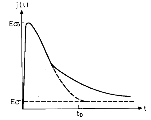
FIG. 38.: Schematic current response of a disordered conductor to an electric field of the form $E(t)=E\Theta(t)$, where $\Theta(t)$ is the step function. For times greater than the diffusion time $t_{d}$, higher quantum corrections lead to log–normal (rather than exponential) decay towards the equilibrium value $E\sigma$. Taken from Ref. [702].

The local density of states $\nu(\vec{r},\epsilon)=-{\rm Im}G^{+}(\vec{r},\vec{r};\epsilon)/\pi$, of particular interest for the metal–insulator transition, was investigated by Lerner, Altshuler, and Kravtsov [703, 689]. In the metallic regime the distribution of $\nu(\vec{r},\epsilon)$ turned out to be Gaussian with log–normal tails, as discussed above for the conductance and the density of states. In the vicinity of the metal–insulator transition, however, the distribution was found to be completely log–normal [703, 689]. Recently, McCann and Lerner [704] showed that this log–normal distribution is linked to multifractal exponents for the cumulants of the local density of states. Multifractal analysis had been pioneered by Wegner [122] who found a whole set of critical exponents for the moments of the inverse participation ratio at the metal–insulator transition, and by Castellani and Peliti [705] who suggested that the electron wave functions at the transition are multifractal. We now describe recent work which has brought multifractal analysis and properties of asymptotic distributions within reach of the non–linear $\sigma$ model.

3 Supersymmetry approaches

Muzykantskii and Khmelnitskii [511] introduced the novel idea that a non–trivial saddle–point configuration of the usual $\sigma$ model in Eqs. (1) and (2) determines the asymptotic tails of the distribution of mesoscopic quantities in one, two, and three dimensions. Starting from Ohm’s law in its time–dependent form,

$$I(t)=\int_{-\infty}^{t}dt^{\prime}\,G(t-t^{\prime})V(t^{\prime})\ ,$$ (168)

these authors expressed the average time–dependent conductance $G(t)$ in terms of the usual supersymmetric functional,

$$G(t)=\int\frac{d\omega}{2\pi}\exp(-i\omega t)\int d[Q]P(Q)\exp(-S[Q])\ ,$$ (169)

where the action $S[Q]$ is given by Eq. (2). The classical (Drude) term has been suppressed. The next steps can probably be best understood when viewed as arising from a saddle–point approximation with respect to both $Q$ and $\omega$ of the combined action

$$S_{\rm comb}[Q,\omega]=-\frac{\pi\nu}{8}\int{\rm trg}[D(\nabla Q)^{2}+2i\omega LQ]d^{d}r+i\omega t\ .$$ (170)

Variation of Eq. (170) with respect to $\omega$ yields the “self–consistency equation” [511]

$$\int\frac{d^{d}r}{V}{\rm trg}[LQ]=\frac{4t\Delta}{\pi}\ .$$ (171)

Variation with respect to $Q$ under the constraint $Q^{2}=1$ leads to an equation reminiscent of the Eilenberger equation [706] for dirty superconductors,

$$2D\nabla(Q\nabla Q)+i\omega[L,Q]=0\ .$$ (172)

This saddle–point approximation should not be confused with the one necessary to derive the $\sigma$ model of Eqs. (1) and (2). While the latter restricts the $Q$ matrices to the coset space with $Q^{2}=1$, the present one fixes the spatial variation of the $Q$ matrices within this coset space. The matrix equation (172) as well as Eq. (171) can be reduced to two equations involving only one scalar function $\theta(\vec{r})$ [511]. Boundary conditions on $\theta$ determine the solutions for $d=1,2$ and $3$.

Two different regimes are distinguished by values of the parameter $t\Delta$ which defines the size of the r.h.s. of the self–consistency equation (171). Physically, $t\Delta$ determines whether individual states in the mesoscopic probe can be resolved. For $t\Delta\ll 1$ and with $t_{D}$ the diffusion time, $G(t)$ is proportional to $\exp(-t/t_{D})$, irrespective of the dimensionality. In the opposite limit $t\Delta\gg 1$ the results depend on $d$. For $d=1$ one finds $G(t)\propto\exp(-g\ln^{2}(t\Delta))$ and for $d=2$, $G(t)\propto(t\Delta)^{-g}$. Here $g$ is the dimensionless conductance. These results do not apply for arbitrarily long times because beyond a certain limit, $t>t^{*}$, the diffusion approximation was found to break down [511]. In this extremely asymptotic regime the function $\theta$ fluctuates on a scale exceeding the elastic mean free path: The spatial derivative obeys $\theta^{\prime}>1/\ell$, and this contradicts the conditions under which $\theta$ is constructed. Therefore, the ultra–long time limit in $d=1,2$ and the regime $t\Delta\gg 1$ in $d=3$ seemed to be inaccessible and the comparison with the results of Altshuler, Kravtsov, and Lerner [689] was inconclusive.

Mirlin [707] observed, however, that the regime $t>t^{*}$ can be reached if the additional constraint $\theta^{\prime}<1/\ell$ is taken into account in solving Eqs. (171) and (172). This modifies the boundary conditions employed in Ref. [511]. For a two–dimensional disk of radius $R$ Mirlin found the following asymptotic behavior in time,

$$G(t)\propto\exp\left(-\frac{\pi\beta g}{4}\frac{\ln^{2}(t/g\tau)}{\ln(R/\ell)}\right)\qquad\qquad(t\Delta\gg(R/\ell)^{2})\ .$$ (173)

This expression agrees exactly with the (slightly amended) result of Ref. [689].

The calculation of eigenfunction statistics, in particular the distribution of eigenfunction components, in the framework of the supersymmetric non–linear $\sigma$ model has been pioneered by Fyodorov and Mirlin [398, 676, 708, 520, 709]. We have already mentioned some of their work in Sec. VI D. The main results for the distribution function $f(u)$ of the eigenfunction amplitudes $u=|\psi(\vec{r}_{0})|^{2}$ are the following [709]. We consider the function

$$Y(Q_{0})=\int_{Q(\vec{r}_{0}=Q_{0}}d[Q]\exp(-S[Q])\ ,$$ (174)

where $Q(\vec{r}_{0})=Q_{0}$ is held fixed at the observation point $\vec{r}_{0}$, and the action $S[Q]$ is essentially given by Eq. (2) (see [709] for the precise notational conventions). In the limit of vanishing frequency $\omega$, and for both orthogonal ($\beta=2$) and unitary ($\beta=1$) symmetry, this function depends on $Q_{0}$ only via the radial parameter $\lambda_{1}$, $Y(Q_{0})\rightarrow\tilde{Y}(-2\beta i\nu\omega\lambda_{1})$. In terms of $\tilde{Y}(z)$ the desired distribution functions can be expressed as [398, 708]

$$f(u) = \frac{1}{V}\frac{d^{2}}{du^{2}}\tilde{Y}(u)\hskip 119.50148pt(\beta=2)\ ,$$ (175)

$$f(u) = \frac{2\sqrt{2}}{\pi Vu^{1/2}}\frac{d^{2}}{du^{2}}\int_{0}^{\infty}\frac{dz}{z^{1/2}}\tilde{Y}(z+u/2)\qquad(\beta=1)\ ,$$ (176)

where $V$ is the volume of the system. These general formulas are valid for arbitrary dimension. In the limit of a constant supermatrix $Q$ (zero mode approximation) the functional Eq. (174) becomes equivalent to Gaussian Random Matrix Theory, see Sec. VI A 1. In this case we obtain the Porter–Thomas distribution discussed in detail in Sec. III E 1,

$$f(u) = V\exp(-uV)\hskip 68.28644pt(\beta=2)\ ,$$ (177)

$$f(u) = \sqrt{\frac{V}{2\pi u}}\exp(-uV/2)\qquad\quad(\beta=1)\ .$$ (178)

For quasi 1d systems, the integral in Eq. (174) can be solved exactly [398]. With $x=L/\xi\ll 1$ the ratio of system length and localization length, and the coefficient $\alpha=2(1-3L_{-}L_{+}/L^{2})$, where $L_{-}$ and $L_{+}$ are the distances from $\vec{r}_{0}$ to the sample edges, the distribution function for $y=uV$ reads [398, 676, 520, 709]

$$f^{(\beta=2)}(y) = \exp(-y)\left[1+\frac{\alpha x}{6}(2-4y+y^{2})+\ldots\right]\hskip 56.9055pt(y\leq x^{-1/2})\ ,$$ (179)

$$f^{(\beta=1)}(y) = \frac{\exp(-y/2)}{\sqrt{2\pi y}}\left[1+\frac{\alpha x}{6}(3/2-3y+y^{2}/2)+\ldots\right]\hskip 19.91684pt(y\leq x^{-1/2})\ ,$$ (180)

$$f(y) \propto \exp\left(\frac{\beta}{2}\left[-y+\frac{\alpha}{6}y^{2}x+\ldots\right]\right)\hskip 65.44142pt(x^{-1/2}\leq y\leq x^{-1})\ ,$$ (181)

$$f(y) \propto \exp\left(-2\beta\sqrt{y/x}\right)\hskip 122.34692pt(y\geq x^{-1})\ .$$ (182)

In $d>1$ dimensions only approximate methods to evaluate Eq. (176) are available. Let us define the parameter $\kappa=\sum_{\vec{q}}(2\pi\nu{\cal D}\vec{q}^{\,2}V)^{-1}$, where the summation extends over the eigenmodes of the Laplace operator in the sample. This sum depends strongly on dimensionality. A perturbative treatment of the non–zero modes in Eq. (176) leads to results [520] identical to the first two lines in Eq. (182) with $\alpha x/6$ replaced by $\kappa$.

For large amplitudes $y\geq\kappa^{-1/2}$ perturbative methods are no longer admissible. Falko and Efetov [710] employed a saddle–point approximation similar to the one introduced in Ref. [511] to derive the following result for $d=2,3$,

$$f(y) \propto \exp\left(\frac{\beta}{2}(-y+\kappa y^{2}+\ldots)\right),\qquad\qquad(\kappa^{-1/2}\leq y\leq\kappa^{-1})$$ (183)

$$f(y) \propto \exp\left(-\frac{\beta}{8\kappa}\ln^{d}(\kappa y)\right),\hskip 99.58464pt(y\geq\kappa^{-1})\ .$$ (184)

Here, $\kappa=\ln(L/\ell)/4\pi^{2}\nu{\cal D}$ for $d=2$ and $\kappa\propto(k_{F}\ell)^{2}$ for $d=3$, where $k_{F}$ is the Fermi momentum and $\ell$ the elastic mean free path. In particular it was possible to investigate the inverse participation numbers $u_{n}=\int_{0}^{\infty}u^{n}f(u)du$. By studying the dependence of these quantities on system size one can address the question of multifractality of the wave functions. In two dimensions and for system sizes $L$ smaller than or of the order of the localization length, the multifractal nature of the wave functions had been established numerically [711, 712], with the result

$$t_{n}\propto L^{-\tau(n)-2},\qquad\qquad\tau(n)=(n-1)d^{*}(n)\ .$$ (185)

The fractal dimension $d^{*}(n)\neq 2$ had been found to depend on the moment considered. In Ref. [710], this fractal dimension was derived analytically,

$$d^{*}(n)=2-\frac{1}{\beta}\frac{n}{2\pi^{2}\nu{\cal D}},$$ (186)

together with the corresponding power law decay in the tails of the wave functions

$$|\psi(r_{0}+r)|^{2}\propto r^{-2\mu}\ .$$ (187)

In Eq. (186) the order $n$ of the moment is restricted by the requirement that $d^{*}(n)>0$. The exponent $\mu$ in Eq. (187) is smaller than unity and varies from wavefunction to wavefunction.

We see from Eq. (184) that the asymptotic behavior of $f(y)$ is again logarithmically normal, in close analogy to the distribution functions for the conductance [689, 511, 707] and for the density of states [687, 689] discussed above. What is the origin of all these log–normal tails? Already in the metallic regime, they appear as an early manifestation of localization, and they become more pronounced as one approaches the localized regime. This suggests the following interpretation. Even in the metallic regime there exist rare states which are localized. As we approach the localized regime, there occur rare states with abnormally strong localization. The log–normal tails are due to the occurrence of such “atypical states” at any value of $g$. This connection between atypical states and asymptotic distribution functions is an active field of research [709, 713, 714, 715].

In conclusion it is satisfying to see how recent progress in the evaluation of the $\sigma$ model helped to provide strong support for earlier calculations [687, 688, 689] of mesoscopic distribution functions based on a combination of perturbation theory and renormalization group methods.

F Interaction–assisted coherent transport

In 1990, Dorokhov [716] considered particles moving in a strictly one–dimensional random potential. He showed that the localization properties of a pair of particles bound tightly by a harmonic potential differ from those of non–interacting particles. In particular, he predicted a sizeable enhancement of the pair localization length for the case where the pair energy is sufficient to excite high–lying modes of the two–particle system. Four years later, it was suggested by Shepelyansky [717] that the wavefunction of two interacting particles in a one–dimensional disordered chain might extend over a length scale $\xi_{2}$ much larger than the one–particle localization length $\xi_{1}$, irrespective of the sign of the two–particle interaction. Shepelyansky’s result indicated that interactions among electrons might significantly alter or modify our present understanding of transport and localization properties of mesoscopic systems. This important development should be seen in connection with the persistent current problem in Sec. VI B. We recall that this problem has led to the general belief that interactions are vital for the understanding of the equilibrium (i.e. ground state) properties of mesoscopic rings.

Technically, the problem of two interacting particles in a random potential can be mapped onto an effective Hamiltonian which turns out to be a random band matrix with strongly fluctuating diagonal entries. Matrices of this type had not been studied previously, and the two–particle problem is, therefore, also interesting from the point of view of Random Matrix Theory.

1 Idea and scaling picture

Shepelyansky [717] considered the following Schrödinger equation for the two–particle wavefunction $\psi_{n_{1}n_{2}}$ in one dimension,

$$[E_{n_{1}}+E_{n_{2}}+U\delta_{n_{1}n_{2}}]\psi_{n_{1}n_{2}}$$ (188)

$$\qquad+\ V[\psi_{n_{1}+1,n_{2}}+\psi_{n_{1}-1,n_{2}}+\psi_{n_{1},n_{2}+1}+\psi_{n_{1},n_{2}-1}]=E\psi_{n_{1}n_{2}}\ .$$ (189)

Here, $n_{1}$ und $n_{2}$ are the (discrete) coordinates of the first and second electron, respectively, $E_{n_{1}}$ and $E_{n_{2}}$ are on–site energies drawn randomly from the interval $[-W,W]$, $U$ characterizes the strength of the Hubbard interaction, and $V$ is the hopping integral. All lengths are measured in units of the lattice spacing and are, therefore, dimensionless. For $U=0$, and not too strong disorder, the one–particle localization length $\xi_{1}$ in the middle of the energy band is roughly given by $\xi_{1}\approx 25(V/W)^{2}$ [718, 719, 720]. We define the two–particle localization length $\xi_{2}$ as the typical scale on which the two–particle wavefunction decays. It was predicted [717] that in the interacting case,

$$\xi_{2}\approx\frac{1}{32}\left(\frac{U}{V}\right)^{2}\xi_{1}^{2}\ ,$$ (190)

provided $\xi_{1}\gg 1$ and $U/V={\cal O}(1)$. This result is noteworthy in two respects: First, for sufficiently large $\xi_{1}$ (i.e. sufficiently weak disorder) one can have a significant enhancement of $\xi_{2}$ as compared to $\xi_{1}$. Second, since the interaction strength $U$ enters the expression (190) quadratically, the effect does not depend on the sign of the interaction.

A first qualitative numerical confirmation of this effect came from the study of the wave packet dynamics for Eq. (189). The time–dependent quantities $\sigma_{+}=\langle(|n_{1}|+|n_{2}|)^{2}\rangle/4$ and $\sigma_{-}=\langle(|n_{1}|-|n_{2}|)^{2}\rangle$ (characterizing center of mass and relative motion, respectively) are shown in Fig. 39. (The angular brackets denote an average over the wave packet probability distribution at a given time $t$). An enhancement effect is clearly visible.

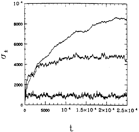
FIG. 39.: Time dependence of the second moments $\sigma_{+}$ and $\sigma_{-}$ defined in the text for $W=0.7$ and $V=1$ and (from top to bottom): $U=1$ ($\sigma_{+}$), $U=1$ ($\sigma_{-}$), and $U=0$ ($\sigma_{+}$). Taken from Ref. [717].

The result (190) was obtained in two rather independent ways. In Ref. [717] the problem was mapped onto the above–mentioned random band matrix with strongly fluctuating diagonal elements which was studied numerically. The result (190) was obtained from a fit to numerical data. Imry [721], on the other hand, invoked a generalization of Thouless’ famous scaling block picture to rederive Eq. (190). We treat both approaches in turn.

It is useful to rewrite Eq. (189) in a basis defined by the single–particle eigenfunctions of the non–interacting part of the system. This yields

$$H_{ij,kl} = (\epsilon_{i}+\epsilon_{j})\delta_{ki}\delta_{jl}+\tilde{Q}_{ij,kl}\ ,$$ (191)

$$\tilde{Q}_{ij,kl} = U\sum_{n}\varphi_{i}(n)\varphi_{j}(n)\varphi_{k}(n)\varphi_{l}(n)\ .$$ (192)

In this representation the Hamiltonian is naturally decomposed into two pieces: a diagonal matrix carrying the eigenvalues $\epsilon_{i}\in[-B,B]$ of the non–interacting system with bandwidth $B\approx 2(2V+W)$, and a non–diagonal matrix $\tilde{Q}_{ij,kl}$ originating from the interaction operator and defined by the overlap of four eigenfunctions $\varphi_{i}$. A typical matrix element $\tilde{Q}$ can be estimated [717] as $\tilde{Q}\approx U/\xi_{1}^{3/2}$.

Since the wave functions $\varphi_{i}$ are localized the Hamiltonian (192) possesses band structure. Shepelyansky used the crucial assumption that all elements of the matrix $\tilde{Q}_{ij,kl}$ in Eq. (192) can be chosen as independent random variables centered at zero. In this way, the Hamiltonian in Eq. (192) is replaced by an effective random Hamiltonian. The latter is the sum of two random matrices: (i) A random band matrix with bandwidth $\xi_{1}^{2}$ and Gaussian distributed elements with variance $U/\xi_{1}^{3/2}$. (ii) A random diagonal matrix with Gaussian distributed elements having variance $B=2(2V+W)$. The addition of the random diagonal matrix to the random band matrix defines a new class of random band matrices. This new class differs significantly from an ordinary random band matrix if the diagonal elements fluctuate much more strongly than the off–diagonal elements. This condition is met in the present case since $\xi_{1}\gg 1$ and $U$ is typically of the order of $V$. Studying the localization properties of the eigenfunctions of this effective Hamiltonian by means of the transfer matrix method, Shepelyansky arrived at the result (190).

In an alternative approach, Imry [721] generalized the ideas of Thouless [517], see Sec. II C, to the two–body problem. He divided the system into blocks of size $\xi_{1}^{2}$. The interaction operator (192) couples the two–particle levels of one block with those of its neighbor. The generalization of the Thouless argument then says: If the “two–particle Thouless energy” $E_{C}^{(2)}$ is larger (smaller) than the two–particle level spacing $\Delta_{2}$ in each of the blocks, the system is conducting (localized), respectively. Using Fermi’s golden rule and the estimate $\tilde{Q}\approx U/\xi_{1}^{3/2}$ given above, Imry obtained $E_{C}^{(2)}=\tilde{Q}^{2}/\Delta_{2}\approx U^{2}/B\xi_{1}$. Here, $B=\Delta_{2}\xi_{1}^{2}$ is the bandwidth which for $\xi_{1}\gg 1$ is proportional to $V$. In analogy to the one–electron case, Imry defined a “two–particle conductance” $g_{2}$ by

$$g_{2}(\xi_{1})=\frac{E_{C}^{(2)}}{\Delta_{2}}=\frac{U^{2}}{B^{2}}\xi_{1}.$$ (193)

For $\xi_{1}\gg 1$ one can clearly have $g_{2}\gg 1$ and the system is far from being localized for electron pairs. Assuming that $g_{2}$ as a function of the length $L$ of the system behaves like a proper conductance, i.e. that $g_{2}(L)\propto L^{-1}$ in one dimension, and using $g_{2}(\xi_{2})\approx 1$ as the definition of $\xi_{2}$, Imry obtained finally

$$\frac{\xi_{2}}{\xi_{1}}=g_{2}(\xi_{1})=\frac{U^{2}}{B^{2}}\xi_{1}\ \ \Leftrightarrow\ \ \xi_{2}=\left(\frac{U}{B}\right)^{2}\xi_{1}^{2}.$$ (194)

Apart from numerical factors which cannot be determined in this approach, the result (190) has been reproduced in a few lines.

2 Microscopic approaches and refinements

Both approaches described above rest on rather important assumptions and approximations. We mention, in particular, the statistical assumptions of the effective random band matrix approach (which are also implicit in the scaling picture, and which neglect all correlations among matrix elements), and the assertion that $g_{2}$ has the scaling behavior of a proper conductance. Therefore, the work of Shepelyansky and Imry was followed by a number of investigations [722, 723, 724] all of which started from the microscopic problem defined by Eq. (189).

Frahm et al. [722] employed the transfer matrix method to solve the Schrödinger equation (189). These authors found that in the parameter range considered, $V=U=1$ and $W=0.7\ldots 2.0$, the two–body localization length behaved as $\xi_{2}\propto\xi_{1}^{\alpha}$ with $\alpha=1.65$. This was the first direct confirmation of the enhancement effect. The exponent $\alpha$ differed from the predicted value $(\alpha=2)$, however. In Ref. [722] this discrepancy was attributed to the strongly non–Gaussian distribution of the interaction matrix elements $\tilde{Q}_{ij,kl}$ in Eq. (192). We will see later, however, that the discrepancy may also be an artifact of fitting an exponent in the crossover regime from $\xi_{2}\propto\xi_{1}$ to $\xi_{2}\propto\xi_{1}^{2}$.

A very direct demonstration of interaction–assisted coherent pair propagation is due to Weinmann et al. [723]. These authors considered a strongly localized, one–dimensional, disordered ring threaded by a magnetic flux. The idea was to identify coherently propagating electron pairs by the periodic flux dependence of their eigenvalues. The period should be given by $h/2e$ instead of $h/e$, the value for single electrons. Indeed, many states with $h/2e$ admixtures were found in Ref. [723], some of them with almost perfect $h/2e$ periodicity. The associated wave functions showed the characteristic “cigar shape” expected when a pair of typical size $\xi_{1}$ travels coherently over a distance $\xi_{2}$, cf. Fig. 40. This result provided compelling evidence for Shepelyansky’s effect.

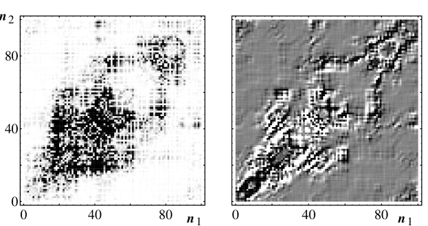
FIG. 40.: A particular two–electron wave function (left) of a one–dimensional, disordered ring and the corresponding local current distribution (right) demonstrating interaction–assisted coherent transport. In the left figure, dark and bright regions indicate high and low probability density, respectively. In the right figure, dark and bright regions indicate local currents in the direction and against the direction of increasing electron coordinates $n_{1}$, $n_{2}$, respectively. Taken from Ref. [723].

A Green function approach introduced by v. Oppen et al. [724] made it possible to investigate in a very efficient way the dependence of the two–particle localization length on the interaction strength $U$. For the problem defined by Eq. (189), a new scaling parameter could be identified. Irrespective of the symmetry of the two–body wave function (Bosons or Fermions), it was found numerically that the ratio $\xi_{2}/\xi_{1}$ depends exclusively on the parameter combination $\mid U\mid\xi_{1}/V$,

$$\frac{\xi_{2}}{\xi_{1}}=\frac{1}{2}+c\frac{\mid U\mid}{V}\xi_{1},$$ (195)

where $c$ is a number of the order $10^{-1}$. It is remarkable that the dependence on $U$ is linear instead of quadratic as predicted in Refs. [717, 721]. Attempts to explain this result are discussed further below. Equation (195) implies that asymptotically, $\xi_{2}\propto\xi_{1}^{2}$, in contrast to the exponent $\alpha=1.65$ found in Ref. [722]. The obvious explanation suggested by Eq. (195) is that the results of Ref. [722] apply only in the crossover region where the dependence of $\xi_{2}$ on $\xi_{1}$ changes from linear to quadratic.

It would be very desirable to have information on the enhancement effect in $d>1$ dimensions. Because of the metal–insulator transition and the question how the mobility edge might be affected by coherent pair propagation, data for $d>2$ dimensions would be of particular interest. However, direct simulations for $d=3$ run into severe numerical difficulties since the size of the basis grows with the linear dimension $N$ like $N^{6}$. The only numerical information on the delocalization effect for $d>1$ comes from simulations of the kicked rotor model by Borgonovi and Shepelyansky [725, 726]. If in a $1d$ model, the time dependence of the perturbing kick is modeled as the superposition of $\nu$ periodic oscillations with incommensurate frequencies, the resulting problem corresponds to a hopping model in $d=\nu+1$ dimensions. A similar correspondence for the case of two interacting kicked rotors can be used to study two interacting particles in higher dimensions. The gain in numerical efficiency is impressive. It amounts to a factor $N^{4}$ [726]. Two cases were investigated. They correspond to an interacting pair in effective dimensions $d_{\rm eff}=2$ and $d_{\rm eff}=2.5$, respectively. The main results of Refs. [725, 726] can be summarized in terms of the behavior of two quantities, $\sigma_{+}$ and $\sigma_{-}$, defined as the distance travelled by the pair and as its typical size, respectively. For $d_{\rm eff}=2$, a saturation of $\sigma_{+}$ as function of time was observed. In the case $d_{\rm eff}=2.5$, however, $\sigma_{+}$ grew without saturation even in a regime where single particles are localized. This was a first numerical indication that pairs might be delocalized earlier than single particles. The numerical data in Ref. [726] also confirmed qualitative arguments in Ref. [725]. It had been predicted that the size of the diffusing electron pairs grows logarithmically with time, while their motion is, correspondingly, slightly subdiffusive: the diffusion constant is inversely proportional to $\ln^{\mu}t$, with $\mu$ of the order of 1.

The linear dependence (195) of $\xi_{2}$ on the interaction strength $U$ was addressed again in a recent study by Weinmann and Pichard [146]. Equations (193) and (194) show that it suffices to investigate the $U$–dependence of the two–particle Thouless energy $E_{C}^{(2)}$. Analytical arguments and numerical simulations [146] show that for system sizes of the order of $\xi_{1}$, there are two regimes for $E_{C}^{(2)}$: a linear ($E_{C}^{(2)}\propto U$) and a quadratic one ($E_{C}^{(2)}\propto U^{2}$). The crossover occurs for $E_{C}^{(2)}\approx\Delta_{2}$. Unfortunately, this result does not directly lead to the appropriate scaling parameter $|U|\xi_{1}/V$, and additional statistical assumptions are necessary to explain Eq. (195) [146]. Analytical investigations of this problem in the framework of a suitable random matrix model were performed by Guhr and Müller–Groeling [261], who derived a novel analytical expression for the spectral two–point correlation function. Jacquod, Shepelyansky, and Sushkov [727] have pointed out that the linear $U$–dependence should only apply close to the band center of the two–particle problem. In all other regions of the spectrum they predict an essentially quadratic dependence of $\xi_{2}$ on $U$.

We have seen that the problem of two interacting particles in a random potential naturally leads to a random band matrix with strongly fluctuating diagonal elements. This class of random matrices generalizes the ordinary random band matrices studied in the context of chaotic quantum systems and transport in quasi 1d wires [139, 673, 674, 398]. It has led to partly [728] and fully [729, 730] analytical work on the properties of the following ensemble of matrices,

$$H_{nn^{\prime}}=\eta_{n}\delta_{nn^{\prime}}+\zeta_{nn^{\prime}}/\sqrt{2b+1}\quad\quad(n,n^{\prime}=1,...,N)\ .$$ (196)

Here, $b$ is the bandwidth and $\eta_{n}$ and $\zeta_{nn^{\prime}}$ are uncorrelated random variables. In Ref. [728] the $\eta_{n}$’s were drawn from the interval $[-W_{b},W_{b}]$ and the $\zeta_{nn^{\prime}}$’s from $[-1,1]$ provided that $|n-n^{\prime}|\leq b$. Otherwise, $\zeta_{nn^{\prime}}=0$. In Refs. [729, 730] the distribution of the $\eta_{n}$’s was rather arbitrary but characterized by a strength $W_{b}$ while the $\zeta_{nn^{\prime}}$’s had a zero–centered Gaussian distribution with variance $\overline{|\zeta_{nn^{\prime}}|^{2}}=(1+\delta_{nn^{\prime}}(\beta-2))A_{nn^{\prime}}/2$. Here $A_{nn^{\prime}}$ differs from zero essentially only in the interval $|n-n^{\prime}|\leq b$ where it has the typical value unity. In both cases, the typical size of the variables is given by the parameter $W_{b}$ and by unity, respectively.

In Ref. [728], two main results for the regime $1\ll W_{b}<\sqrt{b}$ were established by analytical arguments and numerical simulations: (i) For a fixed unperturbed state with energy $\eta_{n}$, the local density of states $\rho_{n}(E)=(1/\pi)\overline{G_{nn}^{+}(E)}$ is always of Breit–Wigner form,

$$\rho_{n}(E)=\frac{\Gamma/2\pi}{(E-\eta_{n})^{2}+\Gamma^{2}/4},$$ (197)

where $\Gamma=\pi/3W_{b}$. (ii) The scale defined by the localization length $\xi=b^{2}/2W_{b}^{2}$ differs from the one set by the inverse participation ratio $\xi_{\rm IPR}=\langle(\sum_{n}|\psi_{\lambda}(n)|^{4})^{-1}\rangle_{\lambda}=b^{2}/4W_{b}^{4}$, where $\psi_{\lambda}(n)$ is an eigenfunction of the Hamiltonian (196) and $\langle...\rangle_{\lambda}$ denotes a spectral average. This means that typical wave functions have very strong site–to–site fluctuations (We recall that the ensemble (196) is of interest only if $W_{b}\gg 1$).

Simultaneously and independently, Fyodorov and Mirlin [729] and Frahm and Müller–Groeling [730] investigated the ensemble (196) by means of the supersymmetric non–linear $\sigma$ model. In these papers, the findings in Ref. [728] were analytically confirmed and extended. In addition to the localization length $\xi$ and the local density of states $\rho_{n}(E)$, the full set of generalized inverse participation ratios $P_{q}=\sum_{n}|\psi_{n}^{(k)}|^{2q}$, and the distribution of the eigenvector components were calculated. These latter quantities were shown to be connected with those for ordinary random band matrices by an appropriate rescaling with a factor $\rho_{n}(E)/\bar{\rho}$ [729, 730], where $\bar{\rho}$ is the average density of states. Specialization of these results to the cases considered in Ref. [728] confirmed all major results obtained there.

A variant of the Hamiltonian ensemble (196) was used by Frahm, Müller–Groeling, and Pichard [731, 732] to investigate the pair dynamics in arbitrary dimension. Generally speaking, the main result of these papers was the analytical proof that the concepts familiar from transport theory of non–interacting electrons also apply mutatis mutandis to the case of electron pairs. A supersymmetric non–linear $\sigma$ model for the two–point function of the effective Hamiltonian was derived. Under omission of source terms, the result is

$$Z_{\rm pair} = \int d[Q]\exp(-S_{\rm pair}[Q])\ ,$$ (198)

$$S_{\rm pair}[Q] = -\frac{\Gamma^{2}B_{2}}{8B_{0}^{2}}\int dR\,{\rm trg}(\nabla_{R}Q)^{2}-i\frac{\pi}{4}\omega\,h\left(\frac{\Gamma}{\omega}\right)\rho_{0}(E)\int dR\,{\rm trg}(QL)\ .$$ (199)

Here, $B_{0}$ and $B_{2}$ are numbers characterizing the band structure of the Hamiltonian, $\rho_{0}(E)$ is the density of unperturbed (non–interacting) states, and $\Gamma$ is the interaction–induced spreading width of these states at the scale $\xi_{1}$. The function $h(\Gamma/\omega)$ is defined in Ref. [731, 732]. Equation (198) must be compared with the corresponding expression for transport of non–interacting electrons in metals [44] introduced in Sec. VI A 1,

$$Z = \int d[Q]\exp(-S[Q])\ ,$$ (200)

$$S[Q] = -\frac{\pi\nu}{8}\int{\rm trg}\left[{\cal D}(\nabla Q)^{2}+2i\omega LQ\right]dr\ .$$ (201)

Here, the scaling parameter of localization theory is the conductivity $\sigma=\nu{\cal D}$. It is clear that Eqs. (198) and (201) are very closely related. This led to the following statements: (i) The effective “conductivity” $\sigma_{\rm eff}=\nu_{\rm eff}(\omega)D_{\rm eff}(\omega)\approx U^{2}\xi_{1}^{2}/W_{b}^{2}$ of the pairs plays exactly the same role as the one–particle quantity $\sigma$. This rigorously justifies Imry’s scaling approach [721]. For $d=1$ one has $\sigma_{\rm eff}\propto\xi_{2}$ so that Eq. (190) is recovered. (ii) The mean quadratic displacement of the pairs increases weaker than linearly, $\langle R^{2}(t)\rangle\propto t/\ln(\Gamma t)^{d}$ for some time scale so that the pairs move subdiffusively. This confirms numerical findings [725, 726] discussed above. (iii) It is possible to define a pair Thouless energy $E_{C}^{(2)}$ below which the spectral statistics of the diffusing pair states is of Wigner–Dyson type. For energy scales larger than $E_{C}^{(2)}$ one recovers the Altshuler–Shklovskii regime [184].

In summary, we have seen that in its essentials, Shepelyansky’s discovery, the phenomenon of interaction–assisted coherent transport of pairs of particles, has been corroborated by a wealth of subsequent work.

3 Finite particle density

The problem of two interacting particles addressed in the previous paragraph is academic, at least for electrons. Indeed, in the many–body case the exclusion principle may prevent virtual transitions into states which are essential for coherent pair propagation. Hence it is necessary to study coherent pair propagation at finite particle density. Only two papers have so far (partly) addressed this important issue [721, 733]. In Ref. [733], von Oppen and Wettig considered two interacting quasiparticles above the Fermi surface in one dimension. Formally, the only difference to previous work was the blocking of all single–particle states up to the Fermi energy $E_{F}$. The interaction of particles within the Fermi sea with each other and with the two quasiparticles was not taken into consideration. It is argued [733] that this procedure amounts to a low–density approximation. It was found that slightly above $E_{F}$, the quasiparticle pair was localized on the scale $\xi_{1}$. With increasing excitation energy the enhancement effect was eventually recovered, but the energy scale for this to happen is given by the bandwidth. This result appears to rule out the possibility to observe coherent pair propagation in an experiment at low temperature in one dimension. Imry [721] has emphasized that the situation might be more favorable in higher dimensions. He argued that for $d=3$ the mobility edge for pairs could be located below the mobility edge for single particles. Let $\epsilon_{m1}$ and $\epsilon_{m2}$ be the excitation energies of the mobility edges for single particles and pairs, respectively. Then, according to Ref. [721],

$$\epsilon_{m2}\propto\epsilon_{m1}^{\tilde{\nu}d/2}\ ,$$ (202)

where $\tilde{\nu}$ is the critical exponent defined by $\xi_{1}\propto\epsilon_{m1}^{-\tilde{\nu}}$. Invoking the Harris criterion [734], $\tilde{\nu}d/2>1$, it is clear that $\epsilon_{m2}\to 0$ faster than $\epsilon_{m1}$, as claimed.

Much more work is necessary to clarify the phenomenon of interaction–assisted coherent transport in many–body systems. The whole field is rather new and progresses rapidly. The most recent developments include a detailed study of the enhancement mechanism in 1d [735], a numerical investigation [736] of two quasiparticles in 2d and 3d, and an unfortunate controversy concerning the role of finite size effects [737, 738].

G RMT in condensed matter physics — a summary

To conclude our overview over developments in condensed matter physics where RMT has played a significant role we now try to summarize and judge the importance and prospects of RMT in this field.

The most direct and therefore also historically first application of RMT in solid state theory was to spectral fluctuations. Roughly, we can distinguish two periods: One in which research focussed on proving the validity of Wigner–Dyson (WD) statistics for some range of parameters, and a second one where efforts were concentrated on identifying deviations from this universal limit. Thus, WD statistics was first established as a valid means of description and then used as a standard of reference. Identifying the limits of validity of WD statistics in the description of spectral fluctuations has turned out to be very fruitful. It has led to a better understanding of the various regimes (clean, ballistic, ergodic, diffusive, critical, and localized) in mesoscopic physics. In this context the $\sigma$ model has served at least two purposes. First, it provided the proof that an ergodic regime with WD type of spectral correlations exists and, second, it turned out to be the proper tool to calculate a number of corrections to this result. We have seen that such corrections were also discovered with the help of diagrammatic perturbation theory and/or scaling arguments. The discovery of a third class of spectral statistics at the mobility edge (different from both RMT and Poisson statistics) poses an interesting challenge: The construction of a stochastic Hamiltonian which reproduces critical spectral fluctuations. Although experimental verification of the theoretical predictions seems to be out of reach for years to come, finding such an ensemble would undoubtedly improve our understanding of the mobility edge. An interesting recent step in this direction is due to Kravtsov and Muttalib [739].

Persistent currents in mesoscopic rings are closely connected with spectral fluctuations. It is therefore natural to expect RMT to play an important role in this problem, too. However, the contribution of RMT to the persistent current problem has been comparatively moderate so far, for several reasons. Initially, one of the main problems was a conceptual one: How to calculate averages in the canonical ensemble. When this question had been answered and first perturbative results had become available, non–perturbative calculations based on RMT did provide the complete and singularity–free solution of the persistent current problem for non–interacting electrons at zero temperature. This was an interesting technical achievement, but it did not alter the discrepancy between theory and experiment. Moreover it is now widely held that the important effect to be understood is the interplay between disorder and electron–electron interactions. Unfortunately this task is at present beyond the scope of RMT. One may speculate that the embedded ensembles investigated some 20 years ago in nuclear physics could one day prove useful.

Applications of RMT to transport in quasi 1d systems have been particularly successful. The paradigm “quasi 1d wire” has united three formerly separate research activities, the random transfer matrix approach, the random Hamiltonian approach of the IWZ model, and random band matrices. Within well–defined limits these three approaches are indeed equivalent. The random transfer matrix method illustrates that RMT is not restricted to modeling the Hamiltonian of a system. This fact has been known at least since Dyson introduced the circular ensembles of $S$ matrices. For spectral problems the distribution of eigenvalues and, thus, a modeling of the Hamiltonian are of central importance. In transport problems, on the other hand, it is the distribution of transmission coefficients that matters. These coefficients are directly related to the eigenparameters of the transfer matrix. The ensemble of random transfer matrices corresponding to an ensemble of disordered quasi 1d wires therefore appears to offer the most direct approach to transport properties. However, an important and sometimes decisive advantage of the Hamiltonian formulation is its great flexibility. Any modification of the system under study is defined in terms of its Hamiltonian and there is absolutely no question about how to incorporate this change into the Hamiltonian formalism. It is far less obvious how the transfer matrix has to be adapted to such a modification. The autocorrelation function of the conductance versus magnetic field strength illustrates this point. This quantity can easily be formulated within the Hamiltonian approach and has been calculated in the diffusive regime. A similar treatment is, unfortunately, still missing in the framework of the transfer matrix approach.

Techniques of the $\sigma$ model have proven to be particularly valuable. Both the equivalence of the transfer matrix approach and the IWZ model, and the relation between random band matrices and quasi 1d wires were established with this technique. Random band matrices are found to play the same role for quasi 1d systems as do the Gaussian ensembles for zero–dimensional systems like atoms, molecules, nuclei, or quantum dots. It is of interest to ask whether generic ensembles of random matrices exist which model properties of higher–dimensional systems.

Problems in $d>1$ dimensions have taken center stage in recent work on the non–linear $\sigma$ model. A systematic improvement of techniques has led from the zero–dimensional case (with perturbative corrections) to exact solutions in quasi 1d systems and, via the recently discovered non–trivial saddle–point solutions, to substantial progress in the understanding of two– and higher–dimensional systems. It has been possible to establish contact with, and to reproduce results of, earlier perturbative renormalization group calculations. This is the most recent success of a program which goes ever further beyond the universal limit of the Gaussian ensembles.

Another step towards more general matrix ensembles has been taken in the context of interaction–assisted coherent pair propagation. The effective Hamiltonian describing two particles in a 1d random potential turned out to be a random band matrix with strong fluctuations on the diagonal. The necessity to introduce a new matrix ensemble originated from the presence of both disorder and interactions. The disorder defines the diagonal entries (localized states) while the interaction induces couplings between these basis states. Again, the $\sigma$ model turned out to be the appropriate tool to investigate the newly defined ensemble. Differences and similarities between ordinary band matrices and those with strongly fluctuating diagonal elements could be identified, leading to an improved understanding of coherent pair propagation. It would be desirable to extend this work and to construct a matrix ensemble which correctly accounts for generic features of Hamiltonians with one– and two–body operators. The improved understanding of the interplay between disorder and interactions might also be helpful in the persistent current problem.

We have seen that RMT has found wide applications in condensed matter physics. These applications go far beyond the scope of the original Gaussian ensembles. In this development, the supersymmetry method has been an invaluable tool. Mapping a random matrix model or a microscopic, effective Hamiltonian onto a non–linear $\sigma$ model reduces the physical content to its very essence: Seemingly dissimilar models turn out to be equivalent, at least in certain regimes. Several examples were mentioned above. The supersymmetry approach is also useful to establish the correspondence between dynamical localization in the kicked rotor and Anderson localization in a thick metallic wire, or to show that interaction–assisted propagation of pairs can be described in terms similar to one–particle diffusion. The list can be continued. Still, there are many open questions. We have mentioned phenomena for which no adequate matrix model has been constructed up to now. Doing so remains a challenge for the future.

VII Field theory and statistical mechanics

In previous sections (Secs. I to III) of our review we have dealt with the history and with mathematical aspects of RMT. With this insight into the foundations and the scope of RMT the subsequent applications to many body physics (Sec. IV), quantum chaos (Sec. V), and disordered systems (Sec. VI) probably came as no surprise. In the present section we discuss the importance of RMT for fields of physics which at first sight seem to have little in common with the more obvious fields of applications just mentioned. In particular we summarize the relation of RMT to interacting Fermions in one dimension (Sec. VII A), to QCD (Sec. VII B), and to field theory and quantum gravity (Sec. VII C). The existence of these “exotic” relations once again demonstrates the universality and ubiquity of RMT.

A RMT and interacting Fermions in one dimension

A deep-lying connection exists between classical Random Matrix Theory and special systems of interacting Fermions in one dimension. This fact was first demonstrated in work by Calogero [740] and by Sutherland [741]. Recently, Simons, Lee, and Altshuler [189, 742] have extended this result to the case of correlation functions. This important work has led to a whole network of connections between different branches of physics. Moreover, it has made it possible to calculate the (hitherto unknown) time–dependent correlation functions of such Fermionic systems using RMT.

We consider the $N$–particle Hamiltonian

$$H_{C}=-\frac{\hbar^{2}}{2m}\left[\sum_{i=1}^{N}\frac{\partial^{2}}{\partial\lambda_{i}^{2}}-\frac{\beta}{2}(\beta-2)\sum_{i<j}\frac{1}{(\lambda_{i}-\lambda_{j})^{2}}\right]+\sum_{i}V(\lambda_{i})$$ (1)

where the position of particle $i$ with $i=1,\ldots,N$ in one dimension is given by $\lambda_{i}$. It was shown by Calogero [740] that $H_{C}$ is integrable provided the potential is Gaussian, $V(\lambda_{i})\propto\lambda_{i}^{2}$. Moreover, for this choice of $V$ the ground state of $H_{C}$ defines a probability distribution $P_{N\beta}(\{\lambda_{i}\})$ of the particle positions $\lambda_{i}$ which coincides [740] with the joint probability density $P_{N\beta}(\{\epsilon_{i}\})$ for the rescaled eigenvalues $\epsilon_{i}$ (see below) with $i=1,\ldots,N$ of the three Gaussian ensembles with $\beta=1,2,4$. The positions $\lambda_{i}$ have to be measured in units of the mean interparticle distance. There is a certain freedom in defining the statistics of the particles described by Eq. (1). Without entering into a detailed discussion we will think of these particles as spinless Fermions.

Putting the confining potential $V(\lambda_{i})$ equal to zero and constraining the motion of the $N$ particles to a circle leads to the Sutherland Hamiltonian [741]

$$H_{S}=-\frac{\hbar^{2}}{2m}\left[\sum_{i=1}^{N}\frac{\partial^{2}}{\partial\lambda_{i}^{2}}-\frac{\beta}{2}(\beta-2)\left(\frac{\pi}{N}\right)^{2}\sum_{i<j}\frac{1}{\sin^{2}[\pi(\lambda_{i}-\lambda_{j})/N]}\right]\ .$$ (2)

The square of the ground–state wave function of $H_{S}$ is equal to the equilibrium distribution of Dyson’s circular ensembles. In the limit $N\to\infty$ the correlation functions of the Hamiltonians (1) and (2) are expected to coincide. We focus attention on the Sutherland Hamiltonian.

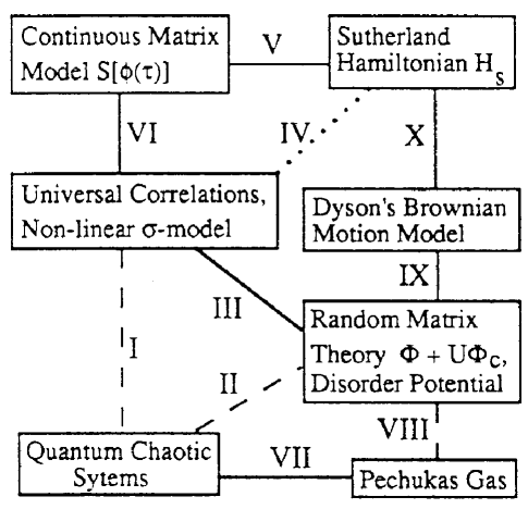
FIG. 41.: Connections between various branches of physics. Taken from Ref. [743].

To formulate the conjecture made in Ref. [189, 742] we recall some results concerning parametric correlation functions of RMT, see Sec. III H 2. We consider the random Hamiltonian

$$H(U)=H_{1}+UH_{2}\ ,$$ (3)

where $H_{1}$ belongs to one of the three Gaussian ensembles, and where $H_{2}$ is a fixed traceless matrix drawn from the same ensemble. The dimensionless parameter $U$ measures the strength of the perturbation $H_{2}$. The eigenvalues $E_{i}$ of $H$ are obviously functions of this strength, $E_{i}=E_{i}(U)$. To display universal aspects of the correlation between the eigenvalues, it is necessary to rescale both $U$ and the $E_{i}$. This is done by defining the rescaled eigenvalues $\epsilon_{i}=E_{i}/\Delta$ where $\Delta$ is the mean level spacing, and the rescaled strength

$$u^{2}=\left\langle\left(\frac{\partial\epsilon_{i}(U)}{\partial U}\right)^{2}\right\rangle U^{2}.$$ (4)

The resulting universal expressions for the level–density autocorrelation functions have been given in Sec. III H 2, see Eq. (215). Simons, Lee, and Altshuler [189, 742] conjectured that these universal functions coincide with the time–dependent particle density correlation functions of $H_{S}$. To establish such a connection, one must identify differences in imaginary time $\tau$ and position $\lambda$ with those in perturbation strength $u$ and energy $\omega$ according to the rules

$$u^{2}=2\tau,\qquad\qquad\omega=\lambda\ .$$ (5)

The first evidence for the conjecture came from expansions of the time–dependent particle density correlation functions $k_{\beta}(\lambda,\tau)$. To leading order in $\tau$ and $1/\tau$, respectively, these functions were shown to agree with the corresponding limits of the level–density autocorrelators (215). Subsequent investigations by the same authors [744, 743] and by Narayan and Shastry [745] established the equivalence of both types of correlation functions exactly. At the same time, Simons and coworkers [744, 743] set up and completed a network of interrelations between different branches of physics that is schematically shown in Fig. 41. We explain and summarize the various connections in the sequel.

The link between the Sutherland Hamiltonian and the universal parametric correlations of Random Matrix Theory has been established in three different ways. First, there are the asymptotic expansions of $k_{\beta}(\lambda,\tau)$ just mentioned (connection IV in Fig. 41). These expansions provide a very direct link between the two fields but are not exact and, in addition, restricted to those correlators for which explicit expressions are known. In practice, these are the two–point correlators. Second, it can be shown that both $H_{S}$ and the non–linear $\sigma$ model for the universal correlators are related to a continuous matrix model introduced in Refs. [744, 743] (connections V and VI). Third, Dyson’s Brownian motion model can be invoked to relate $H_{S}$ with the random matrix Hamiltonian (3) and consequently also with the universal correlations (connections III, IX, and X). We will treat the two exact approaches in turn. In a final paragraph we briefly summarize important new results for 1d Fermions.

1 Continuous matrix model

Following Refs. [744, 743] we consider the partition function

$$Z = \int D\Phi(\tau)\exp\left(-S[\Phi(\tau)]\right)$$ (6)

$$S[\Phi(\tau)] = \frac{1}{\hbar}\int_{-\infty}^{\infty}d\tau\,{\rm tr}\left[\frac{m}{2}\left(\frac{\partial\Phi(\tau)}{\partial\tau}\right)^{2}+V(\Phi)\right]$$ (7)

describing the propagation of $N\times N$ random matrices $\Phi$ from one of the Gaussian ensembles in a potential $V(\Phi)$. The Hamiltonian corresponding to the path integral (7) reads

$$H={\rm tr}\left[-\frac{\hbar^{2}}{2m}\left(\frac{\delta}{\delta\Phi}\right)^{2}+V(\Phi)\right]\ .$$ (8)

With the help of the diagonalization $\Phi(\tau)=\Omega(\tau)\Lambda(\tau)\Omega(\tau)^{\dagger}$ the “Laplacian” $\delta/\delta\Phi$ in Eq. (8) can be separated into radial ($\Lambda$) and angular ($\Omega$) degrees of freedom,

$$\left(\frac{\delta}{\delta\Phi}\right)^{2}=\sum_{i}\frac{1}{J(\lambda_{i})}\frac{\partial}{\partial\lambda_{i}}J(\lambda_{i})\frac{\partial}{\partial\lambda_{i}}+Y(\Omega,\lambda_{i})\ .$$ (9)

Here $J(\lambda_{i})=\prod_{i<j}|\lambda_{i}-\lambda_{j}|^{\beta}$ is the Jacobian known from Random Matrix Theory. In the limit $N\to\infty$ the angular part $Y(\Omega,\lambda_{i})$ can be neglected, and we arrive at the Hamiltonian $H_{C}$ of Eq. (1) provided (i) the potential $V(\Phi)$ does not depend on angular degrees of freedom and (ii) a factor $[J(\lambda_{i})]^{1/2}$ is absorbed into the wavefunctions. Such a connection between an $N$–Fermion Hamiltonian and a continuous matrix model had originally been discussed by Brezin, Itzykson, Parisi, and Zuber [746]. In particular, ground–state expectation values of $H_{C}$ can be expressed in terms of the path integral (7),

$$\langle 0|\ldots|0\rangle=Z^{-1}\int D\Phi(\tau)\ldots\exp(-S[\Phi(\tau)])\ .$$ (10)

The proof of equivalence between the time–dependent $m$–point ground–state correlators of $H_{C}$ (or, equivalently, $H_{S}$) and the $m$–point level–density autocorrelation functions of the random matrix model of Eq. (3) is carried out as follows [744, 743]. Supersymmetric non–linear $\sigma$ models are derived for both types of quantities in the large–$N$ limit. The two non–linear $\sigma$ models are shown to coincide.

The $m$–point ground–state correlators of $H_{C}$ are given by

$$\langle 0|f_{m}(\{\lambda_{\alpha},\tau_{\alpha}\})|0\rangle=\left\langle 0\left|\prod_{\alpha=1}^{m}{\rm tr}\left(\frac{1}{\lambda_{\alpha}^{\pm}-\Phi(\tau_{\alpha})}\right)\right|0\right\rangle.$$ (11)

The quantities $f_{m}$ can be expressed in a standard way in terms of a supersymmetric generating function,

$$Z_{m}(\{\lambda_{\alpha},\tau_{\alpha},J_{\alpha}\})=\int d[\psi]\exp\left[i\psi^{\dagger}(\hat{\lambda}-\hat{\Phi}(\tau)+\hat{J}I)\psi\right]\ .$$ (12)

According to Eq. (10), calculating the ground–state expectation value of $Z_{m}$ amounts to averaging over $\Phi(\tau)$ with the probability density $\exp(-S[\Phi(\tau)])$. Since we are intersted in the universal large–$N$ limit of the correlation functions we can restrict ourselves to the Gaussian case and choose $V(\Phi)\propto{\rm tr}\,\Phi^{2}$. Then the average can be trivially performed. As in other derivations of a non–linear $\sigma$ model, subsequent steps involve [744, 743] a Hubbard–Stratonovich transformation and a saddle–point approximation. The final expression in terms of $4m\times 4m$ supermatrix fields reads

$$\langle 0|Z_{m}|0\rangle = \int d[Q]\exp(-F[Q])$$ (13)

$$F[Q] = i\frac{\pi}{2}\sum_{\alpha}{\rm trg}[(\lambda_{\alpha}^{\pm}+J_{\alpha}I)Q_{\alpha\alpha}]+\frac{\pi^{2}\beta}{8\hbar}\sum_{\alpha\beta}|\tau_{\alpha}-\tau_{\beta}|{\rm trg}[Q_{\alpha\beta}Q_{\beta\alpha}]\ ,$$ (14)

where the mean interparticle distance and $\hbar^{2}/2m$ have been set equal to unity. In a similar way, the correlators of the random matrix Hamiltonian (3)

$$f_{m}(\{\Omega_{\alpha},U_{\alpha}\})=\prod_{\alpha=1}^{m}{\rm tr}\left[\frac{1}{\Omega_{\alpha}^{\pm}-H_{1}-U_{\alpha}H_{2}}\right]$$ (15)

can also be represented in terms of a non–linear $\sigma$ model involving the appropriately rescaled parameters $\omega_{\alpha}=\Omega_{\alpha}/\Delta$ and $u_{\alpha}$ (see above). For $m=2$, this $\sigma$ model can be shown to coincide with that of Eq. (14) after the formal replacements

$$\omega_{\alpha}\leftrightarrow\lambda_{\alpha},\qquad\qquad(u_{\alpha}-u_{\beta})^{2}\leftrightarrow 2|\tau_{\alpha}-\tau_{\beta}|/\hbar\ .$$ (16)

For $m=2$, this establishes the correspondence between the two types of correlation functions. For $m>2$ the replacements (16) cannot be realized by a single unique set of transformations $u_{\alpha}=u_{\alpha}(\{\tau_{\beta}\})$. Instead a slightly more complicated argument has to be invoked, see Refs. [744, 743]. This completes the proof in the general case.

2 Use of Dyson’s Brownian motion model

To establish the link between one–dimensional interacting Fermions and universal parametric correlations via Dyson’s Brownian motion model, Narayan and Shastry [745] started from the Calogero Hamiltonian (1) with $V(\lambda_{i})=\lambda_{i}^{2}/4a^{2}$. For imaginary time $\tau=it$, the time–dependent Schrödinger equation involving $H_{C}$ yields for the quantity $P(\{\lambda_{i}\};\tau)=\psi_{0}(\{\lambda_{i}\})\psi(\{\lambda_{i}\};t)$ the Fokker–Planck equation

$$\frac{\partial P(\{\lambda_{i}\};\tau)}{\partial\tau}=\sum_{i}\frac{\partial}{\partial\lambda_{i}}\left[\frac{\partial P}{\partial\lambda_{i}}+\frac{\lambda_{i}}{a^{2}}P\right]-\sum_{i\neq j}\frac{\partial}{\partial\lambda_{i}}\left[\frac{\beta}{\lambda_{i}-\lambda_{j}}P\right]\ .$$ (17)

Here, $\psi_{0}$ is the ground–state wave function of $H_{C}$. To interpret Eq. (17), we may consider the $\lambda_{i}$ as the position coordinates of $N$ classical particles. Then, Eq. (17) describes the dynamics of the Wigner–Dyson Coulomb gas [58], the $N$ particles being confined by a harmonic potential and interacting via a pairwise logarithmic repulsion (connection X).

In a next step, Narayan and Shastry considered the evolution of the eigenvalues of a perturbed random matrix model similar to Eq. (3),

$$H(x)=H_{0}\cos(\Omega x)+V\sin(\Omega x)/\Omega\ ,$$ (18)

where $H_{0}$ and $V$ are drawn from one of the Gaussian ensembles. For any $x$, $H(x)$ is perturbed by $H^{\prime}(x)=\partial H/\partial x$ and the evolution of the eigenvalues $\epsilon_{i}(x)$ can be expressed as a set of first–order differential equations,

$$\frac{d\epsilon_{i}}{dx} = H_{ii}^{\prime}\ ,$$ (19)

$$\frac{dH_{ii}^{\prime}}{dx} = -\Omega^{2}\epsilon_{i}+\sum_{i\neq j}\frac{2|H_{ij}^{\prime}|^{2}}{\epsilon_{i}-\epsilon_{j}}\ ,$$ (20)

$$\frac{dH_{ij}^{\prime}}{dx} = \sum_{k\neq i,j}H_{ik}^{\prime}H_{kj}^{\prime}\left(\frac{1}{\epsilon_{i}-\epsilon_{k}}+\frac{1}{\epsilon_{j}-\epsilon_{k}}\right)+H_{ij}^{\prime}(H_{jj}^{\prime}-H_{ii}^{\prime})\frac{1}{\epsilon_{i}-\epsilon_{j}}\ .$$ (21)

Interpreted classically, these equations describe the dynamics of $N$ point particles at the positions $\epsilon_{i}$ ($i=1,\ldots N$) and constitute the so–called Pechukas gas [172]. With certain assumptions about the properties of irregular systems, in particular their eigenfunctions, Pechukas derived [172] linear level repulsion from the above equations (connection VII). Moreover, the classical system corresponding to Eqs. (21) has been shown to be integrable [172, 174]. In Ref. [745], infinitesimal increments $\delta\epsilon_{i}$ of the eigenvalues $\epsilon_{i}$ were considered. With the identification $x^{2}=2\tau$, the following statistical properties of the $\delta\epsilon_{i}$ could be derived in the large–$N$ limit,

$$\langle\delta\epsilon_{i}\rangle = -\frac{\epsilon_{i}}{a^{2}}\delta\tau+\beta\sum_{i\neq j}\frac{\delta\tau}{\epsilon_{i}-\epsilon_{j}}\ ,$$ (22)

$$\langle\delta\epsilon_{i}^{2}\rangle = 2\delta\tau\ .$$ (23)

After setting $\lambda_{i}=\epsilon_{i}$ these two equations imply the Fokker–Planck equation (17) for the distribution function $P(\{\epsilon_{i}\};\tau)$. This completes connection IX in Fig. 41. Taking into account the close relation between the Hamiltonians (3), (18) and the non–linear $\sigma$ model [44, 187, 188, 192] (connection III), we see that the second exact link between universal correlations and the Sutherland Hamiltonian has been established. Prior to the publication of Ref. [745], Beenakker [185] already noticed the relation between the universal parametric correlators and Dyson’s Brownian motion model within the hydrodynamic limit.

Finally, it remains to comment on the connections I, II, and VIII in Fig. 41. The corresponding lines are dashed because one has to assume ergodicity, i.e. the equality of the ensemble average in Random Matrix Theory and the running average over energy in a real microscopic system. In many cases this hypothesis has been checked numerically. Numerical confirmations for connection I include the case of quantum billiards [187, 188, 192], hydrogen in a magnetic field [481], and strongly correlated many–particle systems [747]. Connection II is also based on numerical evidence, and connection VIII is discussed in Ref. [57].

3 Further results

The calculation of the dynamical density–density correlators for $\beta=1,2$ and $4$ and the discovery of the various relations discussed in the preceding Secs. VII A 1 and VII A 2 have stimulated important further progress in the understanding of interacting Fermions in one dimension. Using the information provided by Simons et al., Haldane [748] conjectured the form of the density–density correlator for the Calogero–Sutherland model for all rational values of $\beta$. In these cases there is, of course, no known relation to Random Matrix Theory. Independently, Minahan and Polychronakos [749] used group–theoretical arguments to guess the two–point density correlator for integral values of $\beta/2$. Even earlier, Haldane and Zirnbauer [750] calculated the retarded part of the single–particle Green function for $\beta=4$ and later [751] extended their results to $\beta=1$ and to the advanced part. Haldane’s conjecture was proven by Ha [752] with the help of the theory of Jack polynomials [753]. At the same time Ha extended the results derived in Refs. [750, 751] to arbitrary rational $\beta/2$, thus confirming another conjecture by Haldane [754]. Forrester [755] seems to have been the first author to introduce methods involving Jack polynomials in the present context. He, too, used such methods [756] to prove Haldane’s second conjecture.

This shows how new results in Random Matrix Theory have eventually led to novel dynamical correlation functions for a whole class of interacting Fermion systems.

B QCD and chiral Random Matrix Theory

During the last few years, RMT has been applied successfully to certain aspects of quantum chromodynamics (QCD). More precisely, some properties of data generated from lattice gauge calculations have been shown to agree with RMT predictions. This is true, in particular, for level correlation functions and for low–energy sum rules. Other data like those on the chiral phase transition have been semiquantitatively reproduced by RMT. These discoveries are important, and have generated much interest, because they show that QCD possesses generic features. RMT is expected to be the ideal tool to identify and quantify such features. Thus, application of RMT to lattice QCD data will hopefully help to separate the generic from the system–specific properties, and to identify the latter. The work was pioneered by Verbaarschot and his colleagues at Stony Brook. Our references are incomplete. Fairly complete lists can be found in Refs. [757, 758].

Lack of space forces us to treat this topic but briefly, without paying attention to the historic development, and without attempting to put these developments into the overall context of QCD. We confine ourselves to a description of those aspects which are most relevant for RMT. We show evidence that lattice data do have generic features (Sec. VII B 1),

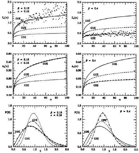
FIG. 42.: Comparison of lattice data and RMT predictions for the number variance $\Sigma_{2}$, for the $\Delta_{3}$ statistic, and for the nearest neighbor spacing distribution $p(s)$. Left: Wilson Fermions, right: Kogut-Suskind Fermions. Taken from Ref. [759].

we sketch the connection between QCD and RMT and introduce the chiral ensembles (Sec. VII B 2), we describe the application of chiral Random Matrix Theory (chRMT) to the chiral phase transition (Sec. VII B 3), and we mention some current lines of interest and open problems (Sec. VII B 4).

1 Evidence for generic features

The first piece of evidence comes from studies of the spectrum of the Euclidean (and Hermitean) Dirac operator

$$iD/=i\partial/+g\frac{\lambda^{a}}{2}A/$$ (24)

for massless Fermions. Here, $g$ is the coupling constant, the matrices $\lambda^{a}$ are the generators of the gauge group, and $A/$ are the gauge fields.

Kalkreuter [760] has calculated the spectrum of $iD/$ for an $SU(2)$ gauge theory on the lattice, both for Wilson and for staggered Fermions. These data have been used to calculate the NNS distribution $p(s)$ and the $\Delta_{3}$ statistic (cf. Eqs. (76) and (83)). The results are shown and compared with chRMT predictions in Fig. 42, taken from Ref. [759]. (The symmetry of the Dirac operator on the lattice differs from the case of the continuum. Wilson and staggered Fermions correspond to the chGOE and chGSE, respectively, both defined in Sec. VII B 2). The agreement is impressive. It shows that the spectral fluctuation properties of the Dirac operator are generic. Somewhat unfortunately, these properties have virtually no bearing on physical observables in QCD.

Another universal property (absent in classical RMT) occurs because the spectrum of $iD/$ is symmetric about zero. The operator $iD/$ anticommutes with $\gamma_{5}$ and the eigenvalues $\lambda_{n}$ therefore occur in pairs $\pm\lambda_{n}$ with opposite signs. Thus, level repulsion should affect directly the average spectral density $\rho(\lambda)$ near zero energy ($\lambda=0$) in a generic way. Here, $\rho(\lambda)$ is defined as

$$\rho(\lambda)=\langle\sum_{n}\delta(\lambda-\lambda_{n})\rangle.$$ (25)

The average (indicated by angular brackets) is taken over all gauge field configurations. The weight factor is the exponential of the Euclidean action. The expected generic dependence of $\rho(\lambda)$ on $\lambda$ near $\lambda=0$ has direct consequences for QCD because the value of $\rho(0)$ is related to the vacuum expectation value $\langle\overline{q}q\rangle$ of the chiral condensate by the Banks–Casher formula $\langle\overline{q}q\rangle=-\pi\rho(0)/V$ where $V$ is the space–time volume. Chiral symmetry is broken if $\langle\overline{q}q\rangle$ is finite (non–zero). In this case, $\rho(0)\sim V$, and the spacing of eigenvalues is $\sim 1/V$ rather than $\sim 1/V^{1/4}$ as would be the case for a non–interacting system. Chiral symmetry is restored for $\rho(0)=0$.

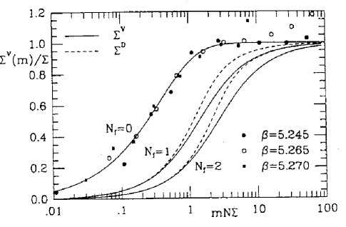
FIG. 43.: Dependence of the chiral condensate on the quark mass. Dots: Lattice data. Solid curve: RMT prediction. Taken from Ref. [761].

First evidence in favor of this assertion (universality of $\rho(\lambda)$ near $\lambda=0$) came from the Leutwyler–Smilga sum rules [762] for the eigenvalues $\lambda_{n}$. For any integer $k$, the sum rules yield closed expressions for $V^{-2k}\sum_{n}\lambda_{n}^{-2k}$. This sum can in turn be written as an integral over $\rho(\lambda)$. It was shown [16] that the sum rules can be derived from chRMT. Moreover, it was conjectured that the microscopic limit $\rho_{S}(z)=\rho(z/(V|\langle\overline{q}q\rangle|))/(V|\langle\overline{q}q\rangle|)$ of the spectral density, obtained by rescaling the argument by $1/(V|\langle\overline{q}q\rangle|)$, should in the thermodynamic limit be a universal function. This conjecture was validated when it was shown [761] that lattice results for the dependence of the chiral condensate on the mass of the valence quarks can be reproduced using the chRMT result for $\rho_{S}$ as the only input, see Fig. 43.

Perhaps the most compelling evidence so far for the universality of $\rho(\lambda)$ near $\lambda=0$ is obtained from a comparison of lattice data for staggered Fermions in the quenched approximation with chRMT predictions. The lattice calculations were performed for strong coupling ($\beta=4/g^{2}=2.0$) and for four different lattice

FIG. 44.: Microscopic spectral density (upper row) and distribution of the smallest eigenvalue of the Dirac operator for four different lattice sizes. The histograms represent lattice data, the dashed curves correspond to chRMT predictions. Taken from Ref. [763].

sizes $V=L^{4}$ with $L=4,6,8$, and $10$, resulting in 9979, 9953, 3896, and 1416 configurations, respectively [763]. The comparison is shown in Fig. 44. Higher correlation functions also display universal features.

2 Chiral random matrix ensembles

The chiral random matrix ensembles can best be introduced by writing the Euclidean Dirac operator of Eq. (24) in matrix form. We choose a chiral basis (consisting of eigenstates of $\gamma_{5}$). In this basis, $iD/$ only couples states of opposite chirality and has the form

$$\left[\matrix{0&iD/\cr(iD/)^{\dagger}&0}\right]\ .$$ (26)

This suggests defining a random matrix model with matrices of the form

$$\left[\matrix{0&W\cr W^{\dagger}&0}\right]$$ (27)

where $W$ is a random matrix. In the chiral random matrix models, the average over gauge fields with the exponential of the Euclidean action as weight factor is replaced by the average over the matrices $W$ with a suitable weight factor $P(W)$ as in Sec. III A 1. Normally, $P(W)$ is chosen as a Gaussian. The limit $N\rightarrow\infty$ of the dimension $N$ of $W$ is taken.

Depending on the symmetry of $iD/$ (which must be reflected in the symmetry of $W$), there are [764] three chiral ensembles, in complete analogy to Sec. III A 1. They depend on the number $N_{c}$ of colors and on the representation (fundamental [f] or adjoint [a]) of the Fermions. The chiral Gaussian unitary, orthogonal and symplectic ensembles are defined, respectively, and apply as follows: (i) chGUE ($W$ complex): for [f] and $N_{c}\geq 3$, (ii) chGOE ($W$ real): for [f] and $N_{c}=2$, and (iii) chGSE ($W$ real quaternion): for [a] and $N_{c}\geq 2$. In the case of lattice calculations with $SU(2)$ gauge symmetry, the chGOE (the chGSE) applies for Wilson Fermions (for staggered Fermions, respectively).

The chiral random matrix ensembles differ from the classical ensembles introduced in Sec. III A 2 mainly in their behavior near $\lambda=0$. As a consequence of the chiral symmetry of $iD/$, in these ensembles the point $\lambda=0$ plays a special role, and the translational symmetry of the classical ensembles is broken. Near $\lambda=0$ there is repulsion of pairs of eigenvalues of opposite sign. This causes $\rho_{S}(x)$ to become generic. A very similar mechanism operates in the unitary ensemble describing Andreev scattering, see Sec. VI A 2. By way of example, we give here the form of $\rho_{S}(x)$ for the chGUE. It depends on the number $N_{f}$ of flavors and on the topological charge $\nu$,

$$\rho_{S}(x)=\frac{x}{2}\left(J_{N_{f}+\nu}^{2}(x)-J_{N_{f}+\nu+1}(x)J_{N_{f}+\nu-1}(x)\right)\ .$$ (28)

The special role of the point $\lambda=0$ does not, however, affect the form of the NNS distribution $p(s)$, or of the $\Delta_{3}$ statistic which in the bulk are the same as for the classical ensembles, see Fig. 42.

3 The chiral phase transition

As shown in Sec. VII B 1, for zero quark masses chiral random matrix models yield a non–zero value of the chiral condensate. This describes the spontaneous breaking of chiral symmetry at zero temperature. Two models have been put forward which modify Eq. (27) in such a way that temperature is included in a schematic way [765, 766, 767, 768]. These models aim at a description of the chiral phase transition. In both models, a temperature–dependent diagonal matrix $D$ is added to $W$ in Eq. (27).

What happens qualitatively to $\rho(\lambda)$ as $D$ is increased, starting from $D=0$? We focus attention on the global properties of $\rho$ and disregard the local suppression of $\rho$ at $\lambda=0$ displayed in Sec. VII B 1. In the simplest case where $D$ is a multiple of the unit matrix, $D=D_{0}{\bf 1}_{N}$, two limiting cases are obvious. At $D_{0}=0$, $\rho(\lambda)$ has the shape of a semicircle. For $W=0$ and $D_{0}>0$, on the other hand, all eigenvalues have values $\pm D_{0}$. Keeping $D_{0}$ fixed and increasing $W$ from $W=0$ will lift the degeneracy of eigenvalues of fixed sign and generate two semicircles with identical radii and with centers at $\pm D_{0}$. The two semicircles do (do not) overlap if their radii are smaller (bigger) than $D_{0}$. We now apply these insights to the chiral phase transition. We use the fact that according to the Banks–Casher formula, the chiral condensate is proportional to $\rho(0)$. We keep $W$ fixed and increase $D_{0}$, starting from $D_{0}=0$. The semicircle becomes deformed. At the value of $D_{0}$ where it splits into two semicircles, $\rho(0)$ vanishes, and the chiral phase transition occurs. This is basically the mechanism employed in both Refs. [765, 768].

We have discussed this point in some detail because it shows that in describing the chiral phase transition in terms of chRMT, use is made of the semicircle law, not one of the generic properties of chRMT. And the critical exponents for the phase transition are determined by the shape of the semicircle at the end of the spectrum. Is this procedure trustworthy? Several authors have investigated non–Gaussian probability distributions $P$ for classical RMT, where $P(H)$ has the form $\exp(-{\rm tr}V(H))$ with $V(H)$ some polynomial, see Sec. VIII. It was found that in the limit of infinite dimension, the spectra are generically confined to a finite interval, and that the behavior of the mean level density near the end points is always of semicircle type. More precisely: Near the end point $a$ of the spectrum, the mean level density $\rho(E)$ behaves like $(E-a)^{\alpha}$ with $\alpha$ a rational number between zero and one. This lends support to the models of Refs. [765, 768]. Still, it must be kept in mind that RMT does not necessarily give a correct prediction of the details of the chiral phase transition.

The two models mentioned above differ in detail. In Ref. [765], the temperature is included schematically in the form of the lowest Matsubara frequency, and $D$ is accordingly chosen as $\pi T{\bf 1}$. With $T_{c}$ the critical temperature, the temperature dependence of the chiral condensate $\langle\overline{q}q\rangle(T)$ is given by $\langle\overline{q}q\rangle(T)=\langle\overline{q}q\rangle(0)\sqrt{1-(T/T_{c})^{2}}$. The chiral phase transition is of second order with mean field critical exponents. The inclusion of all Matsubara frequencies [766, 767] yields very similar results. In the model of Ref. [768] (which was inspired by the instanton liquid model), a fraction $\alpha$ of the diagonal elements of $D$ vanishes (with $0\leq\alpha\leq 1$ trivially), while the rest has identical values $d$. Both $\alpha$ and $d$ are (unknown) monotonically increasing functions of $T$. For a phase transition to occur, $\alpha$ must be equal to one, and $d$ must exceed a critical value $d_{c}$. The order as well as the critical exponents of the chiral phase transition depend on the way in which $\alpha$ and $d$ approach $1$ and $d_{c}$, respectively. A comparison between these results and lattice and/or instanton model calculations may shed light on the temperature–dependence of $\alpha$ and $d$.

4 Current lines of research and open problems

The field is still quite young. Yet, a fair number of papers has appeared. For recent reviews see Refs. [757]. Aside from the topics mentioned above, these papers have addressed the following points. (a) The spectrum of the Dirac operator at finite temperature [769]; (b) the calculation of $k$–point functions at finite $T$ (with $k>2$) [770] (c) the finite volume QCD partition function for finite quark masses [771]; (d) the spectrum of the lattice Dirac operator for Wilson Fermions; (e) inclusion of the chemical potential in chRMT [772, 773, 774, 775]. The last point is probably the most difficult but also the most challenging because on the lattice, unquenched calculations with a chemical potential seem beyond reach. As mentioned above, this list is incomplete.

C Random matrices in field theory and quantum gravity

After some preliminary remarks (Sec. VII C 1) we briefly explain the use of topological concepts and RMT in general field theory (Sec. VII C 2) before we discuss the special example of two–dimensional quantum gravity in Sec. VII C 3.

1 Preliminary remarks

In the stochastic models discussed through most of this review, random matrices were used successfully to simulate generic properties of the Hamiltonian or of a scattering matrix in a quantum problem described by the Schrödinger equation. In Sec. VII B we have seen that this substitution also works for certain aspects of relativistic quantum mechanics where the Dirac equation applies. Demonstrative experiments present strong evidence for the usefulness of this same procedure in the study of classical wave phenomena, see Sec. V D. This holds true, in particular, for electromagnetic waves which, in three dimensions, are described by a vectorial Helmholtz equation, and for elastomechanical waves which are described by Navier’s equation.

We now turn to stochastic models where the use of random matrices has a different origin. The representative examples given below stand for a whole class of problems where it is the fields — rather than the Hamiltonian or another linear operator — which are replaced by an ensemble of random matrices. Often, the replacement has topological reasons. Cases in point are field theory (Sec. VII C 2), and quantum gravity in two dimensions (Sec. VII C 3). Although differently motivated, these random matrix models are, at least on the formal and on the mathematical level, often closely related to the ones discussed in other sections of this review. Because of this connection, a fruitful transfer of insights and methods between both areas exists. We expect that in future years this transfer will become even stronger in both directions.

2 Planar approximation to field theory

Consider a non–Abelian gauge theory with internal symmetry group $SU(N)$. We treat $N$ as a parameter and study the limit of large $N$. Such a study is motivated by quantum chromodynamics where the gauge group is $SU(3)$ because quarks come in three colors. In the absence of exact solutions for $SU(3)$, it is hoped that the results for large $N$ might be of help.

A useful classification of the diagrams generated by the perturbation expansion of the field theory in powers of the coupling constant uses topological concepts. Surfaces can be classified topologically in terms of their genus. For instance, a sphere has genus $h=0$, a torus has genus $h=1$, etc. The diagrams are classified by the minimum genus of the surface needed to draw them. Diagrams with genus zero are called planar. It was shown by ’t Hooft [776] that the asymptotic expansion of the field theory in inverse powers of $N$ yields terms which correspomd exactly to this topological classification. Only planar diagrams survive in the limit $N\rightarrow\infty$, provided the coupling constant is properly scaled with $N$. The higher order terms in $1/N$ correspond to non–planar diagrams which have to be drawn on surfaces of genus $h$ higher than zero.

The generality of this result suggests that a model study of the expansion of field theories might be very useful. Brezin et al. [746] studied models for the planar approximations of $\varphi^{3}$ and $\varphi^{4}$ theories. We focus here on the $\varphi^{4}$ theory. In a $d$-dimensional space $x_{\mu},\mu=1,\ldots,d$ such a theory is defined by a Lagrangean of the type

$${\cal L}=\partial_{\mu}\varphi\partial_{\mu}\varphi+\frac{1}{2}\varphi^{2}+\tilde{g}\varphi^{4}$$ (29)

where $\tilde{g}$ is the coupling constant. A model for this theory is obtained by replacing the field $\varphi(x)$ with a Hermitean $N\times N$ matrix $M(x)$. The model Lagrangean reads

$${\cal L} = {\rm tr}\left(\partial_{\mu}M\partial_{\mu}M\right)+V(M,g)$$ (30)

$$V(M,g) = \frac{1}{2}{\rm tr}M^{2}+\frac{g}{N}{\rm tr}M^{4}\ .$$ (31)

The global invariance group of this Lagrangean is the group $SU(N)$. Thus, it is possible to study the planar limit by taking the limit $N\rightarrow\infty$ while the parameter $g$ is held fixed. The Feynman rules for the diagramatic expansion of this matrix model in powers of $g$ involve the two matrix indices and are a straightforward extension of those for scalar or vector fields. To make plausible the explicit occurrence of the factor $1/N$ in the coupling constant $g/N$, we refer to the discussion in Sec. VIII where more general non–Gaussian weight factors with a polynomial potential in the exponent will be considered. Within this model one can generically solve the so-called counting problem, i.e. one can find the number $E^{(d)}(g)$ of connected planar vacuum diagrams of a given order in $g$ in $d$ dimensions. We discuss this for $d=0$ and $d=1$.

In zero dimensions, each diagram is unity, apart from an overall weight. This implies [746] that, up to a $g$-independent normalization constant, $E^{(0)}(g)$ can be obtained from the large–$N$ limit of the expression

$$\exp\left(-N^{2}E^{(0)}(g)\right)=\int d[M]\exp\left(-V(M,g)\right)\qquad(N\to\infty)$$ (32)

with the usual flat measure $d[M]$. To connect to standard random matrix theory, the integrand can be viewed as a non–Gaussian probability density. For large $N$, the normalization integral yields the counting function versus $g$. It is shown in Ref. [746] that this counting function coincides with the one of the $\varphi^{4}$ theory. In the large–$N$ limit, there are no contributions due to the matrix structure of the fields $M$.

Using the $U(N)$ invariance of the integrand, we reduce the problem to integrations over the eigenvalues $\lambda_{n},n=1,\ldots,N$ where the squared Vandermonde determinant $\Delta_{N}^{2}(\lambda)$ appears in the integrand. To compute the large–$N$ limit of Eq. (32), the method of steepest descent is used and yields saddle–point equations for the eigenvalues $\lambda_{n}$. The counting function $E^{(0)}(g)$ is approximated by the logarithm of the integrand of the right hand side of Eq. (32) taken at these saddlepoints. In a proper continuum limit, the resulting sums are replaced by integrals. This yields

$$E^{(0)}(g)=\int_{-2a}^{+2a}d\lambda u(\lambda)\left(\frac{1}{2}\lambda^{2}+g\lambda^{4}\right)-\int_{-2a}^{+2a}d\lambda u(\lambda)\int_{-2a}^{+2a}d\lambda^{\prime}u(\lambda^{\prime})\ln|\lambda-\lambda^{\prime}|$$ (33)

(34)

where $u(\lambda)$ is the mean level density, and where $-2a$ and $+2a$ with $a=a(g)$ are the end points of the spectrum. The first term on the right hand side of Eq. (34) is due to the potential $V(M,g)$, the second one, due to the Vandermonde determinant. The factor $1/N$ in the coupling constant in Eq. (30) has disappeared. This is because the continuum limit involves a rescaling of the eigenvalues by a factor of $\sqrt{N}$. Brezin et al. [746] find an explicit result for $u(\lambda)$. In the limit $g=0$, this result reduces to the Wigner semicircle law. Hence, a closed expression for the counting function $E^{(0)}(g)$ is obtained. In the planar limit, the coefficients of an expansion of $E^{(0)}(g)$ in powers of $g$ give the desired combinatorical factors.

For $d=1$ the planar approximation provides an interesting connection to the Calogero–Sutherland Model and related theories, see Sec. VII A. We replace the Lagrangean of Eq. (30) by the Hamiltonian and quantize the latter. This yields

$${\cal H}=-\frac{1}{2}\Delta+V(M,g)$$ (35)

where the kinetic term is the usual Laplacian in matrix space,

$$\Delta=\sum_{n=1}^{N}\frac{\partial^{2}}{\partial M_{nn}^{2}}+\frac{1}{2}\sum_{n<m}\left(\frac{\partial^{2}}{\partial{\rm Re}^{2}M_{nm}}+\frac{\partial^{2}}{\partial{\rm Im}^{2}M_{nm}}\right)\ .$$ (36)

It can be shown [746] that for large $N$, the counting function $E^{(1)}(g)$ is given by the lowest eigenvalue of ${\cal H}$,

$${\cal H}\psi=N^{2}E^{(1)}(g)\psi\ .$$ (37)

The value of $E^{(1)}(g)$ is found by varying the expectation value of ${\cal H}$ with respect to the functions $\psi$ in the limit of large $N$. The ground–state wave function $\psi$ can only depend on the radial degrees of freedom. This is so because the $U(N)$ invariance of the potential $V(M,g)$ implies the condition $\psi(M)=\psi(UMU^{\dagger})$. Hence, $\psi$ is a symmetric function of the eigenvalues $\lambda_{n}$ of $M$. To construct such symmetric wave functions $\psi$, Brezin et al. make the ansatz

$$\psi(\lambda_{1},\ldots,\lambda_{N})=\frac{\omega(\lambda_{1},\ldots,\lambda_{N})}{\Delta_{N}(\lambda)}\ .$$ (38)

The Vandermonde determinant $\Delta_{N}(\lambda)$ is antisymmetric in the eigenvalues $\lambda_{n}$. Since $\psi$ is symmetric, $\omega$ has to be antisymmetric as well. This ansatz reduces the kinetic part of Eq. (35) to the Euclidean Laplacian of the $N$ matrix eigenvalues $\lambda_{n},n=1,\ldots,N$. If, moreover, the interaction is of $\varphi^{4}$ or related type, the Hamiltonian acquires the form of $N$ non–interacting Fermions, described by the antisymmetric wavefunction $\omega(\lambda_{1},\ldots,\lambda_{N})$. This construction yields explicit results for the counting function. It also shows the connection to the Calogero–Sutherland model, see Sec. VII A.

By adding to the potential the terms ${\rm tr}M_{k}M_{k^{\prime}}$, Itzykson and Zuber [130] extended these investigations to $K$ coupled matrix fields $M_{k},k=1,\ldots,K$. In the resulting model, the $U(N)$ invariance is broken. In the case $K=2$, it was possible to integrate analytically over the diagonalizing groups. The result, the famous Itzykson-Zuber integral, was later identified as a special case of a more general formula due to Harish-Chandra [129].

3 RMT and two-dimensional quantum gravity

As in field theory, the use of Random Matrix Theory in two–dimensional quantum gravity is motivated topologically. Again, the basic idea derives from the planar approximation. The starting point is string theory, providing a link to the theory of random surfaces where further applications exist. A review was recently given by Abdalla et al. [777]. Here, we only try to motivate the use of RMT in quantum gravity.

We consider a $d$-dimensional space in which functions $X^{\mu}(\xi_{0},\xi_{1}),\ \mu=1,\ldots,d$ parametrize the position of a string on the two-dimensional world sheet $(\xi_{0},\xi_{1})$. For the description of the string dynamics, it is convenient to use the Polyakov string action [778],

$$S=\frac{1}{2}\int d^{2}\xi\sqrt{|g|}g^{\alpha\beta}\partial_{\alpha}X^{\mu}\partial_{\beta}X_{\mu}\ .$$ (39)

Here $g_{\alpha\beta}(\xi_{0},\xi_{1})$ with $\alpha,\beta=0,1$ is the two–dimensional gravitational field. Minimization of the functional $S$ with respect to the $X^{\mu}$ and to the fields $g_{\alpha\beta}$ gives the correct equations of motion for the string with all required constraints. However, further contributions like a cosmological term have to be added to the action $S$. The partition function of a string action of this type is then given by the functional integral

$$Z=\int D[X]\int D[g]\exp(-S)\ .$$ (40)

The integration over the gravitational field amounts to a summation over all topologies of the two-dimensional surface described by the string. Therefore, the partition function can be expanded in terms of the genus $h$ and the area $A$ of the surface,

$$Z=\sum_{h=0}^{\infty}\kappa_{0}^{2h}\int_{0}^{\infty}dA\exp\left(-\mu_{B}A\right)Z_{h}(A)\ .$$ (41)

Here $\mu_{B}$ is the bare cosmological constant and $\mu_{B}A$ is the cosmological term of the action. The expansion proceeds in powers of the bare string coupling constant $\kappa_{0}$. The expansion coefficients $Z_{h}(A)$ are the partition functions for fixed genus $h$ and area $A$. At this point, the connection to the previous section becomes apparent where the genus expansion was motivated by the topology of diagrams. Hence, the $h=0$ term in Eq. (41) corresponds to a planar approximation.

A way to proceed in actual calculations is to discretize the surfaces of given genus $h$, i.e. the sphere, the torus and so on, using polygons with a fixed number $n$ of edges. Discretized models for

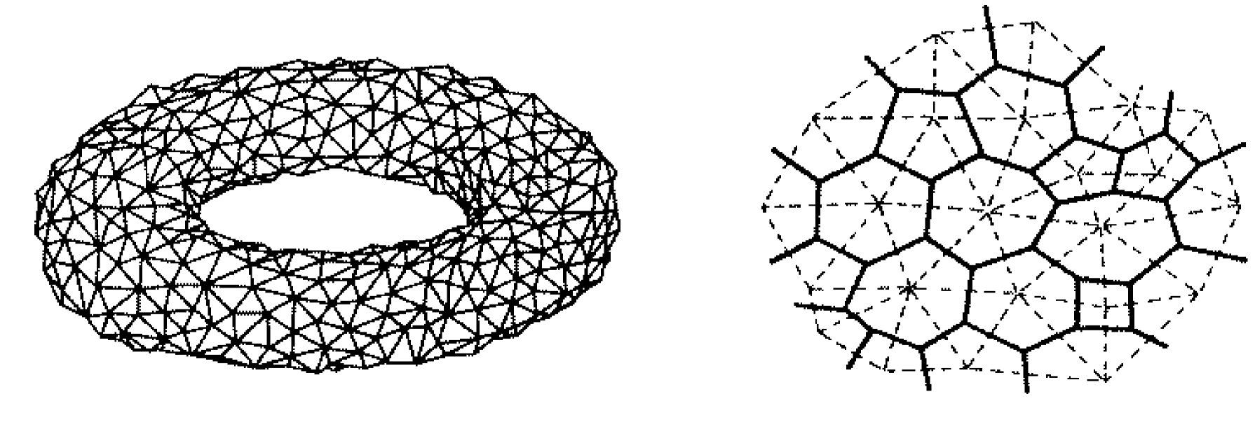
FIG. 45.: Left hand side: A triangulated torus. Right hand side: A piece of a triangulated surface (dashed lines) superposed with its dual (solid lines). Taken from Ref. [777].

random surfaces were introduced by David [779], Kazakov [780] and Ambjørn, Durhuus and Fröhlich [781]. Apparently, these authors were inspired by Regge’s work [782] of 1961. Explicit calculations are often easier in such discretized models than in the continuum version.

The dual graph of a discretization of a surface is defined by connecting the centers of the covering $n$-gons with lines. These dual graphs are typical Feynman graphs of given genus $h$ of a zero-dimensional $\varphi^{n}$ field theory. Thus, the partition functions $Z$ can be approximated in terms of a model of the $\varphi^{n}$ type. A triangulated torus and the dual of a piece of a triangulated surface are shown in Fig. 45. However, certain constraints must be observed. Most importantly, the partition functions $Z_{h}(A)$ in Eq. (41) show a double scaling relation. It turns out that only Hermitean $N\times N$ matrices $M$ meet all the requirements. The resulting matrix model is of the type

$$Z^{\prime} = \int d[\varphi]\exp\left(-N{\rm tr}V(M)\right)$$ (42)

$$V(M) = \frac{1}{2}M^{2}+\sum_{n>2}(g_{n}\Lambda^{(n-2)/2})M^{n}\ .$$ (43)

The $g_{n}$ are coupling constants and $\Lambda$ is associated with the cosmological constant. As in the previous section, an asymptotic expansion in inverse powers of the dimension $N$ effectively yields a diagrammatic genus expansion. The coefficient functions have the desired scaling properties and are identified with the functions $Z_{h}(A)$. The expansion parameter $1/N$ plays the role of the string coupling constant $\kappa_{0}$ in the discretized version of Eq. (41).

VIII Universality

The overwhelming majority of investigations involving invariant random matrix ensembles deals with the Gaussian case (GRMT). However, the requirement that the ensemble should be invariant under appropriate (unitary, orthogonal, or symplectic) transformations in matrix space, admits a much wider class of matrix ensembles with a probability density $P_{N\beta}(H)$ of the form

$$P_{N\beta}(H)=Z^{-1}\exp\left(-{\rm tr}V(H)\right)\ .$$ (1)

Here, $Z^{-1}$ is the normalization constant or inverse partition function. The potential $V(H)$ is arbitrary provided the existence of $Z$ is guaranteed. The Gaussian case corresponds to the choice

$$V(H)=\frac{\beta}{4v^{2}}H^{2},$$ (2)

where $v$ and the elements of the $N\times N$ matrix $H$ have the dimension energy. For other forms of the Gaussian potential typically used in the literature we refer to the discussion at the end of Sec. III A 2. It has been mentioned in the Introduction of this review that the choice (2) is dictated by mathematical convenience rather than by physical principles. Under these circumstances it is necessary and important to ask which statistical properties are generic, i.e. common to all or very many ensembles defined in Eq. (1), and which are specific for the Gaussian case. This is the issue referred to as “universality”.

First convincing numerical evidence in favor of universality was provided by Porter and Rosenzweig [783], see Appendix A.1 of Mehta’s book [23]. These authors calculated the eigenvalue density and the nearest neighbor spacing distribution for the Gaussian probability density and for the densities $P(H_{ij})=(1/2)\Theta(1-|H_{ij}|)$ and $P(H_{ij})=(1/2)(\delta(H_{ij}+1)+\delta(H_{ij}-1))$. In all these cases they found convergence to the semicircle law (eigenvalue densities) and to a curve close to the Wigner surmise (spacing distribution), respectively. For obtaining the semicircle law, statistical independence of the matrix elements is the essentil ingredient. This investigation greatly enhanced the confidence in the usefulness of RMT. From the mathematical point of view, an interesting connection to the theory of free random variables was found by Voiculescu [784].

Orthogonal polynomials [23] provide a powerful analytical tool to investigate Gaussian as well as non–Gaussian ensembles of random matrices. We briefly outline this method. Upon diagonalization of the matrices $H$ one obtains the joint probability density function for the eigenvalues,

$$P_{N\beta}^{(E)}(E_{1},\ldots,E_{N})=Z^{-1}\prod_{i<j}|E_{i}-E_{j}|^{\beta}\exp\left(-\sum_{i}V(E_{i})\right),$$ (3)

where $Z$ is now defined without the integration over angles. We have chosen the energy eigenvalues $E_{i}$ as arguments instead of the dimensionless quantities $x_{i}$, see Sec. III A 2. Equation (3) involves the Vandermonde determinant $\prod_{i<j}(E_{i}-E_{j})={\rm det}[(E_{i})^{j-1}]$. The value of this determinant remains unchanged if the monomials $(E_{i})^{j-1}$ are replaced by arbitrary (but linearly independent) polynomials $p_{n}(E)$ with degrees $n=0,1,\ldots,N-1$. If one chooses these polynomials to be orthogonal in the following sense,

$$\int_{-\infty}^{\infty}dE\exp\left(-V(E)\right)p_{n}(E)p_{m}(E)=\delta_{nm}\ ,$$ (4)

and if one defines the functions

$$\psi_{n}(E)=p_{n}(E)\exp(-V(E)/2)$$ (5)

the joint probability density in the case $\beta=2$, to which we restrict ourselves here, has the form

$$P_{N2}^{(E)}(E_{1},\ldots,E_{N})={\rm det}[K(E_{i},E_{j})].$$ (6)

We have defined the kernel

$$K(E,E^{\prime})=\sum_{i=0}^{N-1}\psi_{i}(E)\psi_{i}(E^{\prime})\ .$$ (7)

In the Gaussian case Eq. (4) defines the Hermite polynomials. All correlation functions

$$R_{\beta k}(E_{1},\ldots,E_{k})\propto\int dE_{k+1}\ldots dE_{N}\ P_{N\beta}^{(E)}(E_{1},\ldots,E_{N})$$ (8)

can now be expressed in terms of this kernel. For the mean density of eigenvalues $\rho(E)\equiv R_{(\beta=2)1}(E)$ and for the connected two–point correlation function $T_{\beta 2}(E,E^{\prime})=\rho(E)\rho(E^{\prime})-R_{\beta 2}(E,E^{\prime})$ we have, in particular,

$$\rho(E) = K(E,E)$$ (9)

$$T_{(\beta=2)2} = [K(E,E^{\prime})]^{2}.$$ (10)

Fox and Kahn [785], Leff [786], and Bronk [787] investigated certain “classical” cases of non–Gaussian potentials $V(E)$, see also chapter 19 in Ref. [23]. The cases studied explicitly include the potentials corresponding via Eq. (4) to the Legendre [786], Laguerre [785, 787], and Jacobi [785, 786] polynomials. In these particular examples the kernel $K(E,E^{\prime})$ was shown to be universally given by

$$K(E,E^{\prime})=\frac{1}{\pi}\frac{\sin(\rho(\hat{E})(E-E^{\prime}))}{E-E^{\prime}}.$$ (11)

in the large–$N$ limit and for $\beta=2$. Performing the limit $N\to\infty$ was made possible by the well–known Christoffel–Darboux formula, see Eq. (20). Given $\hat{E}$, Eq. (11) holds for values of $E$ and $E^{\prime}$ where the mean level density is essentially constant, $\rho(\hat{E})\simeq\rho(E)\simeq\rho(E^{\prime})$. The result (11) implied that after proper rescaling (“unfolding”) of the energy variable, two– and higher–point correlation functions were identical for the classical ensembles, in contrast to the mean level density. As a result, the conjecture [786] that correlations should be “relatively insensitive” to the form of the potential $V(E)$, became highly plausible.

Further significant progress in the universality problem had to wait until 1990. Motivated by problems in two–dimensional quantum gravity (see Sec. VII C), Ambjørn, Jurkiewicz, and Makeenko [788] then discovered a very general and far–reaching result. (We follow the summary in Ref. [789]). We consider a unitary random matrix ensemble with a general polynomial potential

$$V(H)=\sum_{k}\frac{g_{k}}{k}H^{k}\ .$$ (12)

The coefficients $g_{k}$ are essentially arbitrary except that for $N\to\infty$ the mean level density should be non–zero in only one finite interval. Using an expansion of the resolvents in powers of $H$, i.e. a perturbative method, and keeping only terms of leading order in $N^{-1}$, Ambjørn et al. calculated the connected part $G(E,E^{\prime})$ of the two–point Green function in the large–$N$ limit. We remind the reader that a $1/N$ expansion is equivalent to a topological expansion in the genus of the surfaces needed to draw the diagrams of the field theory defined by Eq. (12), see Sec. VII C 2. While Brezin et al. [746] had found that the mean level density $\rho(E)$ does depend on the details of the potential $V(H)$ it was now shown by Ambjørn et al. that $G(E,E^{\prime})$ depends on the potential only through the spectral end points $a$ and $b$. In the special case of a symmetric potential $V(H)=V(-H)$ with $b=-a$, $G(E,E^{\prime})$ is given by [788]

$$G(E,E^{\prime})=\overline{{\rm tr}(E-H)^{-1}\ {\rm tr}(E^{\prime}-H)^{-1}}-\overline{{\rm tr}(E-H)^{-1}}\ \ \overline{{\rm tr}(E^{\prime}-H)^{-1}}=$$ (13)

$$\frac{1}{4(E-E^{\prime})^{2}}\left(-2+\frac{(E^{2}-a^{2})+(E^{\prime 2}-a^{2})}{\sqrt{(E^{2}-a^{2})(E^{\prime 2}-a^{2})}}\right)-\frac{1}{4}\frac{1}{\sqrt{(E^{2}-a^{2})(E^{\prime 2}-a^{2})}}\ .$$ (14)

(15)

The general formula for non–symmetric potentials and an extension to complex rather than Hermitean matrices is also given in Ref. [788]. The general connected n–point Green functions

$$G(E_{1},\ldots,E_{n})=N^{2n-2}\overline{N^{-1}{\rm tr}(E_{1}-H)^{-1}\ldots N^{-1}{\rm tr}(E_{n}-H)^{-1}}^{\,c}$$ (16)

were shown [788] to be also universal in the sense stated above. In addition to the results in leading order, a systematic $1/N^{2}$ expansion of the $n$–point correlators and of the free energy $F={\rm ln}Z/N^{2}$ was developed in Ref. [790],

$$G(E_{1},\ldots,E_{n}) = \sum_{h=0}^{\infty}\frac{1}{N^{2h}}G_{h}(E_{1},\ldots,E_{n})$$ (17)

$$F = \sum_{h=0}^{\infty}\frac{1}{N^{2h}}F_{h}\ .$$ (18)

It was shown that these $1/N^{2}$ corrections are again universal. For symmetric potentials, the corrections to the Green functions are of the form

$$G_{h}(E_{1},\ldots,E_{n})=\frac{R_{h}\left(\{E_{i}^{2}-a^{2}\},\{M_{a}^{(l)}\},a\right)}{\sqrt{\prod_{i=1}^{n}(E_{i}^{2}-a^{2})}}\ .$$ (19)

Here, the $R_{h}$ are rational functions, and the $M_{a}^{(l)}$ are additional parameters, cf. Ref. [789]. Analogous results have also been derived for non–symmetric potentials [790] and complex matrices [791]. Moreover, the statements made above for the two–point Green functions could be generalized [789, 792] to the case where, in the large–$N$ limit, the level density $\rho(E)$ has support in $s$ distinct intervals. For each $s$ a new universality class arises in which the two–point correlators are universal and depend on the potential $V$ only through the end points of the $s$ intervals.

For small distances $|E-E^{\prime}|$, the two–point correlator of Eq. (15) does not yield the universal form (11) of the kernel $K(E,E^{\prime})$. The reason is that the two expressions apply in two different limits. This became particularly transparent in a paper by Brezin and Zee [793] who considered potentials $V(H)$ in the form of even polynomials in $H$. They made an ansatz for the asymptotic (in $n$) form of the associated orthogonal polynomials $p_{n}(E)$ and, hence, for $\psi_{n}(E)$. Knowledge of this asymptotic form is helpful. Indeed, by means of the Christoffel–Darboux identity the kernel $K(E,E^{\prime})$ defined in Eq. (7) can be written as

$$K(E,E^{\prime})=c_{N}\frac{\psi_{N}(E)\psi_{N-1}(E^{\prime})-\psi_{N-1}(E)\psi_{N}(E^{\prime})}{E-E^{\prime}}$$ (20)

with an $N$–dependent constant $c_{N}$. In the large–$N$ limit the ansatz in Ref. [793] and the ensuing expression for $K(E,E^{\prime})$ become exact. Two limiting cases were considered in Ref. [793]. (i) The difference $E-E^{\prime}$ is of order $1/N$ and both energy arguments are at a finite distance from the end points of the spectrum. Then, the universal form (11) holds. Local universality (which of course applies equally to all higher correlation functions) was thus proven for all symmetric potentials of polynomial form. For an extension of this result to more complicated potentials see Ref. [794]. (ii) The difference $|E-E^{\prime}|$ is so large that the number of levels in the interval $E-E^{\prime}$ is of order $N$. Because of this large number, the kernel $K(E,E^{\prime})$ oscillates heavily with changes of $E$ or $E^{\prime}$. Averaging over a finite number of such oscillations in the vicinity of both $E$ and $E^{\prime}$, Brezin and Zee obtained

$$T_{(\beta=2)2}^{\rm smooth}(E,E^{\prime})=\frac{1}{2N^{2}\pi^{2}}\frac{1}{(E-E^{\prime})^{2}}\frac{a^{2}-EE^{\prime}}{\left[(a^{2}-E^{2})(a^{2}-E^{\prime 2})\right]^{1/2}}.$$ (21)

Thus, they rediscovered the universal correlation function (15) of Ambjørn et al. [788]. (The relation between $G(E,E^{\prime})$ and $T_{(\beta=2)2}(E,E^{\prime})$ is simple and explained in Ref. [789]). Apparently, the perturbative calculation of Ref. [788] cannot account for the oscillatory behavior of the level correlations. In Ref. [186], this fact was attributed to an interchange of limits. In a perturbative calculation $N$ is sent to infinity before the poles in the resolvents are placed on the real axis. Therefore the individual poles merge to form a cut and the fine structure is lost. In the method of orthogonal polynomials and in the supersymmetry method (see below), on the other hand, no such problem arises.

We digress and mention some related work although it is not directly related to the subject of this section. In Ref. [186], “time” dependent correlations in a matrix ensemble defined by

$$P[H]=Z^{-1}\exp\left(-\int_{-T}^{T}dt\,{\rm tr}\left[\frac{1}{2}\left(\frac{dH}{dt}\right)^{2}+V[H]\right]\right)$$ (22)

were calculated with diagrammatic techniques. Here, $H=H(t)$ is explicitly a function of time. In particular the (smoothed) current–current correlator $\langle J(E,t)J(E^{\prime},0)\rangle$ for arbitrary $t$ was derived, thus generalizing earlier results by Szafer and Altshuler [183] and by Beenakker [185]. The current operator was defined as $J(E,t)=N^{-1}\sum_{i}(dE_{i}/dt)\delta(E-E_{i}(t))$. In subsequent work [795] these time–dependent correlations were related to the cross correlations between the eigenvalues of two separate (but not independent) Gaussian ensembles. The relationship is very similar to the one described in Sec. VII A 1 between parametric correlations and a continuous matrix model. In Ref. [796] the interesting relation

$$G(E,E^{\prime})=\frac{\partial^{2}}{\partial E\partial E^{\prime}}{\rm ln}\left(\left(\frac{G(E)-G(E^{\prime})}{E-E^{\prime}}\right)+\ldots\right)$$ (23)

was established for arbitrary polynomial $V[H]$. The dots indicate terms that do not contribute to the connected two–point level density correlation function $T_{\beta 2}(E,E^{\prime})$. The result (23) is rather surprising since it connects a universal quantity like $G(E,E^{\prime})$ with the non–universal one–point function $G(E)$. The validity of Eq. (23) could be extended [796] to the case where $H=H_{1}+H_{2}$ with $P[H]=P_{1}[H_{1}]P_{2}[H_{2}]$.

Beenakker [797] gave a particularly simple and elegant derivation of the form (21) of the universal “wide” correlator. At the same time, he could generalize the result to the orthogonal and symplectic cases, and to non–polynomial potentials. Using the functional derivative method which he had developed [652] and applied to the case of the positive spectrum of the transfer matrix, he calculated directly the connected two–point correlation function $T_{\beta 2}(E,E^{\prime})$. We briefly summarize the main steps of the derivation. The two–point function is given by the functional derivative of the eigenvalue density with respect to the confining potential,

$$T_{\beta 2}(E,E^{\prime})=\frac{1}{\beta}\frac{\delta\rho(E)}{\delta V(E^{\prime})}\ .$$ (24)

Here the potential $V$ is arbitrary provided the support of the spectrum remains compact as $N\to\infty$. In this limit, $V$ and $\rho$ are connected by the integral relation

$${\bf P}\int_{a}^{b}dE\frac{\rho(E)}{E^{\prime}-E}=\frac{d}{dE^{\prime}}V(E^{\prime})$$ (25)

where ${\bf P}$ denotes the principal value and $a$ and $b$ are the end points of the spectrum. Variation of Eq. (25) with respect to $V$ and inversion of the result together with Eq. (24) immediately yields a universal expression for $T_{\beta 2}(E,E^{\prime})$. The result is valid for all $a$ and $b$, for $\beta=1,2,4$, and for all $V$. For $a=-b$ and $\beta=2$ it reduces to the known case given by Eq. (21). Extending the methods used in Ref. [790], Itoi [798] also derived explicit expressions for two–point correlators in the orthogonal and symplectic symmetry classes and established the universality of the multi–point correlators.

Hackenbroich and Weidenmüller [799] showed that all local correlation functions (i.e., functions on the scale of the mean level spacing) are independent of the confining potential $V(H)$. This statement holds under the following two provisos: The support of the spectrum must remain finite in the limit $N\rightarrow\infty$, and the arguments of the correlators must be scaled correctly (energy differences are to be expressed in units of the local mean level spacing). The proof applies to all three symmetry classes, and to all types of correlation functions involving level densities, $S$ matrix elements, and/or parametric correlations of arbitrary order. Starting point is the supersymmetric generating functional

$$I=\int d[\Psi]\int d[H]P_{N\beta}(H)\,\exp\left(\frac{i}{2}\Psi^{\dagger}L^{1/2}(H-E+M)L^{1/2}\Psi\right)$$ (26)

for a product of Green functions of $H$. Energy differences, source terms and, if present, the coupling to external channels are all contained in the matrix $M$ [799]. From the fact that $M$ is of order $N^{-1}$ it follows that to leading order in $N^{-1}$, $I$ is a function of the unitary invariants $A_{\alpha\beta}=\sum_{\mu}(L^{1/2}\Psi)_{\alpha\mu}(\Psi^{\dagger}L^{1/2})_{\beta\mu}$ only. Before averaging, these invariants are introduced via an additional double integration over a delta function. In a sense, this step replaces the Hubbard–Stratonovich transformation which applies in the Gaussian case only. Then, the integration over the variables $\Psi$ is carried out. For large $N$, all remaining integrations (including the ensemble average, i.e. the integration over the distribution of $H$) are then evaluated with the help of the saddle–point approximation. Except for the occurrence of the local mean level density $\rho(E)$, the final expression for $I$ coincides with the result for the Gaussian case. This proof derives its elegance from the fact that one never leaves the level of the generating functional. At the same time this is its drawback: The proof reduces the form of the correlators to the Gaussian case but is of no help in actual calculations of the latter.

Freilikher, Kanzieper, and Yurkevich [800, 801] addressed the issue of universality for wide classes of confining potentials (for which the spectrum is bounded). The authors used orthogonal polynomials and mathematical results [802, 803, 804, 805] which partly are quite recent. In the “$\alpha$–ensemble” [806, 807] with $V(E)\propto|E|^{\alpha}$, the orthogonal polynomials are defined [800] with respect to the “Freud weights” [802]. Rigorous results for the kernel $K(E,E^{\prime})$, see Eq. (7), led to the following statements. As $\alpha$ approaches unity from above, the mean level density $\rho(E)$ develops a sharp peak in the center of the spectrum. In contradistinction, all two–point correlators, local as well as smoothed ones, retain their universal form down to and including the value $\alpha=1$. In Ref. [801] the rigorous treatment was extended to the “Erdös–type” of confining potentials which at infinity grow faster than any polynomial, and to the presence of a hard edge in the spectrum of the Hamiltonian. This last condition is motivated by applications involving the (non–negative) eigenparameters of random transfer matrices, see Sec. VI C 2. Again, in all cases considered, the universality of both global (smoothed) and local two–point correlators could be shown.

Explicit and interesting examples for potentials $V(H)$ leading to non–universal statistics were given by Nagao and Slevin [808], and by Muttalib and coworkers [809, 810]. In the spectrum of the generalized Gaussian and Laguerre ensembles (which involve an additional logarithmic term in the potential $V(H)$), there exist domains with non–universal correlations [808]. In Ref. [810], the $q$–dependent potential

$$V(H)=\sum_{n=0}^{\infty}{\rm ln}[1+2q^{n+1}\cosh(2\chi)+q^{2n+2}],\quad H=\sinh\chi$$ (27)

with $q\in[0,1]$ was considered. The spectrum is not bounded (the eigenvalues range from $-\infty$ to $+\infty$). As a function of $q$, the nearest neighbor spacing distribution interpolates between Wigner–Dyson (WD) and Poisson statistics [810]. The orthogonal polynomials corresponding to the choice (27) are the $q$ Hermite polynomials. Potentials related to the $q$ Laguerre polynomials exhibit similar spectral properties [809]. It was conjectured [810] that these properties are shared by the entire family of potentials related to $q$ polynomials [811].

Since they interpolate between WD and Poisson statistics, potentials of the type (27) might be important for the description of the crossover from metallic to localized behavior in mesoscopic systems, see Sec. VI A 2. Another possibility to describe this transition is provided by random matrix ensembles which break the rotational invariance in Hilbert space assumed in Eq. (1). Examples are ensembles of random band matrices (see Sec. VI D) and other ensembles [812, 142] with a preferential basis.

Why do rotationally invariant potentials of the type (27) deviate from universal behavior? Canali and Kravtsov [813] gave an interesting answer: As one goes from the $\alpha$ ensemble ($\alpha\geq 1$) to potentials like (27) which grow only logarithmically with $H$, the $U(N)$ invariance is spontaneously broken. This seems the common feature of all approaches which describe the localization transition in terms of random matrix ensembles.

IX Common concepts

In previous sections of this review, we have encountered numerous examples of successful applications of RMT to physical systems. We have also listed many open problems. Perhaps the most impressive aspect of this discussion is the wide range of topics involved. It suggests that RMT is a universal tool. Indeed, RMT correctly describes fluctuation properties of nonrelativistic and relativistic quantum systems. It applies to chaotic quantum systems with few degrees of freedom, to disordered quantum systems, to classical wave propagation in disordered media, and to many–body quantum systems. RMT also describes spectral fluctuation properties and parametric correlations of several very different wave equations. And RMT connects to quantum gravity and to the Calogero–Sutherland type models in one dimension. In this final section, we focus attention on the ubiquity of RMT.

To this end we first recall the foundation, success and limitations of RMT as well as some of the open problems in the various fields of application.

A Synopsis

(i) Many–body systems. RMT started with Wigner’s attempt to formulate a generic model for the spectral fluctuation properties of complex many–body systems. The Hamiltonian of every such system is assumed to be a member of an ensemble of random matrices. The ensemble is characterized completely by symmetry properties. Apart from appropriate mean values, no detailed knowledge of the system at hand enters the definition of the ensemble. Thus, system–specific features (beyond the mean values needed to define RMT properties) cannot be reproduced and are assumed to be irrelevant for fluctuation properties. This model has been extremely successful in the description of spectral fluctuation properties and of cross–section fluctuations in complex atoms, molecules, and atomic nuclei. This is true in spite of the fact that the interactions between the constituents in these systems are vastly different: Nuclei are bound by the short–range nuclear force which is repulsive at very small distances, atoms and molecules are governed by long–range Coulomb forces. Only states near the ground state seem to display system–specific features. At higher excitation energies, collective and/or single–particle properties may still be present but seem to appear only as gross features. For instance, the giant dipole resonance in nuclei appears as a broad resonance in the $\gamma$–absorption cross section. The spreading width of the resonance is very much larger than the mean level spacing of the many–body system. The resonance does not correspond to a single eigenstate of the nucleus. Similar statements apply to other collective modes. Isobaric analogue resonances in heavy nuclei provide a good example. Hence it now appears that, within each set of conserved quantum numbers and sufficiently far above the ground state, any strongly interacting quantum system with many degrees of freedom must be expected to display fluctuation properties of RMT type of the appropriate symmetry.

Does an energy scale exist in such systems (analogous to the Thouless energy in disordered systems) beyond which RMT ceases to apply? Can we expect to find the analog of localization in the eigenfunctions? As long as the origin of stochastic behavior in such many–body systems is unclear, questions such as these have no easy answer. It is conceivable that stochasticity arises from classical chaos. This is the case in systems with few degrees of freedom. In that case, limitations of RMT similar to the ones to be mentioned under (ii) are expected to apply. It is equally conceivable, however, that stochasticity is an emergent property of strongly interacting systems with many degrees of freedom irrespective of whether the underlying classical dynamics is fully or only partially chaotic. After all, an assumption of similar type (equal a priori occupation probability of all accessible parts of phase space or Hilbert space) has been used with amazing success as the foundation of classical and quantum statistical mechanics. In this case, possible limitations of RMT would have a different origin, and would probably be of different form. The available experimental evidence (covering sequences of up to several hundred levels) does not point to any such limitations at present.

(ii) Classically chaotic systems with few degrees of freedom. The fundamental property of these systems is the instability of the classical trajectories. It leads to stochastic behavior on both the classical and the quantum level. For fully chaotic systems with a single intrinsic time scale, the situation is fairly well understood. We have discussed three attempts, based on semiclassics, the non–linear $\sigma$ model, and structural invariance, respectively, to rigorously establish the Bohigas conjecture. Although a complete proof does not yet exist, the conditions for the occurrence of spectral fluctuations of RMT type are known in their essentials. The energy interval within which fluctuations of RMT type occur, is determined by the shortest periodic orbits. Fully chaotic systems with several intrinsic time scales, such as, e.g., a chain of coupled chaotic billiards, have not been considered in detail in this review. They show fluctuations similar to those of disordered quasi one–dimensional mesoscopic systems and are described by random band matrices. Here, localization phenomena may occur. Generic systems with mixed phase space pose a major challenge. The idea of chaos–assisted tunneling has been very successful. Closer inspection has shown, however, that the structure of classical phase space is quite complex, especially at the interface between regular and chaotic domains. This fact does influence the fluctuation properties. We have emphasized the conceptual importance of model systems (like two coupled harmonic oscillators) for the investigation of many of these questions. Another challenge consists in extending the semiclassical results obtained for systems with two or three degrees of freedom to higher dimensions.

(iii) Disordered systems. Both the origin of stochastic behavior and the limitations of RMT are quite clear in disordered systems. The random distribution of impurity scatterers together with a suitable ergodic theorem furnish an immediate justification for modeling these systems in a stochastic fashion. Such a justification is much more subtle in the cases discussed under (i) and (ii), where stochasticity appears as an emergent property of the many–body dynamics or the classically chaotic dynamics, respectively. For disordered systems, spectral fluctuations and the fluctuations of transport coefficients are – within known limits – of classical RMT type. The applicability of classical RMT is limited to the diffusive regime (if we disregard the extreme ballistic limit where the system becomes a quantum billiard) and, within this regime, to an energy interval given by the Thouless energy. Outside of this interval, and in the crossover to either the ballistic or the localized regime as well as at the mobility edge, other universal laws govern the fluctuation properties. Except for the behavior at the mobility edge, these laws can be derived from suitable generalizations of classical RMT. In this sense, RMT has been found to apply universally to disordered systems, too. We have not been able to dwell on the passage of classical light waves, or of radar waves, through a medium with a randomly varying index of refraction. However, much of what has been said about disordered mesoscopic systems applies here, too. In particular, weak localization occurs and is thus seen to be not a quantum, but a wave phenomenon.

The phenomenon of localization is not limited to disordered systems. As “dynamical localization”, it occurs likewise in chaotic quantum systems. The kicked rotor is the standard example. This system can be mapped onto a one–dimensional non–linear $\sigma$ model. This shows the connection to quasi one–dimensional disordered wires and to RMT.

(iv) Wave equations. Spectral fluctuation properties of RMT type are not linked to a specific linear second–order differential equation (the Schrödinger equation). The spectra of acoustic and elastomechanical waves in irregularly shaped solids show RMT fluctuations, and so do the eigenmodes of Maxwell’s equations in three–dimensional cavities. These phenomena are governed by rather different linear wave equations. In the case of elastomechanical waves even the boundary conditions (vanishing stress tensor) are completely different from those for Schrödinger waves. Another example of a linear wave equation, the Dirac equation, will be mentioned under (v). Moreover, very different interaction potentials in the Schrödinger equation also give rise to RMT fluctuations. We are not aware of any attempts to explain this general applicability of RMT to various wave phenomena in a generic fashion.

(v) Field theory. We have considered two examples, QCD and a $\phi^{4}$ theory involving matrix fields $\phi$. In general, local fluctuation properties are of little interest in these field theories. Nevertheless, it is noteworthy that the spectral fluctuations of the Dirac operator in QCD coincide with RMT predictions, for two reasons. First, here is another example of universality: A first–order differential operator coupled to gauge fields possesses RMT fluctuation properties. Second, the existence of RMT fluctuations shows that the data generated by lattice gauge calculations contain generic features. This fact poses a challenge: To separate the generic features from the physical content, in order both to obtain a better understanding of the problem, and to simplify the calculations.

Certain global features of RMT are also universal. This is true, for instance, for the shape of the global RMT spectrum near the end points, or for the structure of diagrams generated through a loop expansion of the above–mentioned $\phi^{4}$ theory. This is why RMT applies to two–dimensional gravity and thereby establishes a conncection with conformal field theory, and why RMT can be used to model the chiral phase transition of QCD.

B Discussion

This tour d’horizon shows that most applications of RMT to physical systems predict local fluctuations in terms of a system–specific input. The input consists of suitable mean values: Spectral fluctuations require the mean level spacing as input. For cross section fluctuations, the average scattering matrix serves the same purpose. For conductance fluctuations, the mean conductance takes this role. In this sense, RMT predictions are not parameter free: They relate fluctuations to mean values. This statement can be given a different and more interesting form. The mean values can be absorbed into properly rescaled local variables, and RMT predictions for fluctuations and correlation functions acquire universal form. This applies not only to level correlations, but very generally to the dependence of correlation functions on any external parameter (parametric correlations). We have presented many examples where such universal RMT predictions have been tested successfully.

By construction, RMT predictions are based on ensemble averages. On the other hand, variances or correlation functions extracted from a data set are almost always obtained from a running average over a given system. The equality of the results of both averaging procedures is guaranteed by ergodicity. Although not proved in full generality, ergodicity has been shown to hold in a number of cases.

During the last fifteen years, the non–linear $\sigma$ model has become an invaluable tool in RMT. Without this model, the universal features of RMT might never have been discovered to their full extent. Through the medium of field theory, the common statistical properties of chaotic and of disordered systems, and the universality of parametric correlations, have been displayed, and have been cast into compact form. The model has been indispensable also in other contexts. For instance, many aspects of stochastic scattering would not have been accessible without it. And the insight that local RMT fluctuation properties do not depend on the Gaussian distribution of matrix elements finds perhaps the simplest and most general proof through the non–linear $\sigma$ model. The need to calculate some RMT correlation functions has led to a number of extensions of supersymmetry. We think here of new and unconventional saddle points, of Fourier analysis on graded spaces, and of extensions of the Itzykson–Zuber integral. Due to lack of space we could not do justice to some of these developments. These examples show that modern applications of RMT have led to mathematical research which has meanwhile become a field in its own right. The situation is reminiscent of the early days of (classical) RMT where progress was eventually possible due to mathematical input from the theory of orthogonal polynomials.

Are the success and the ubiquity of RMT really surprising? One might argue that RMT is trivial because it only displays the consequences of von Neumann–Wigner level repulsion, i.e. of the simple fact that two states connected by a non–vanishing matrix element repel each other. But this argument fails to take into account all other predictions of RMT which go far beyond simple level repulsion. These predictions derive from the symmetry of the Hamiltonian, and from the postulated invariance properties of RMT which in turn embody the generic aspects of the entire approach. The form of the Vandermonde determinant appearing in the invariant measure of RMT is entirely due to the postulated rotational invariance of the random matrix ensemble in Hilbert space. It is true, of course, that this determinant implies (a particular form of) level repulsion. The degree of repulsion is determined by the symmetry of the Hamiltonian. A simple counting argument leads directly to the exponent $\beta=1,2,4$ in the typical factor $|E_{\mu}-E_{\nu}|^{\beta}$ in the Vandermonde determinant. But the forms of the two–point function $Y_{2}$ and of higher correlation functions, of the $\Delta_{3}$ statistic measuring the spectral stiffness, and of the nearest neighbor spacing distribution are not determined by level repulsion alone and require for their derivation the full rotational invariance of the ensemble. The same is true of the universal form of correlations of observables which depend upon an external parameter. With regard to these observables, RMT possesses genuine predictive power and leads to highly non–trivial results. The results are generic, not based on dynamical principles, and derive only from the underlying symmetry and invariance requirements. Even on a global scale (as opposed to the local scale of the mean level spacing), spectral correlations still display some degree of universality. The extension of RMT to random band matrices and random transfer matrices, important for the understanding of extended systems and localization, breaks rotational invariance. The transition to localization and the ensuing correlation functions are determined by the way in which the influence of the Vandermonde determinant in the invariant measure is gradually neutralized. But even in this domain of application of RMT, generic non–dynamical features remain and are of central interest. They are embodied in the effective Lagrangian of the non–linear $\sigma$ model.

In the end, the universal features of RMT appear to correspond remarkably well to generic properties of quantum (and certain classical) systems. We recall Balian’s proof that among all rotation invariant ensembles Gaussian RMT maximizes the information entropy. These facts seem to imply that in the absence of any further knowledge about the system, Gaussian RMT yields the best approximation to the physical properties of that system.

In spite of this argument, we feel that the universal applicability of RMT remains an amazing fact. It signals the emergence of a theory of wave phenomena, both classical and quantal, which does not relate to dynamical properties. RMT is valid essentially on the local scale defined by the mean level spacing of the system. On larger scales, correlation functions are often used to determine system–specific properties. The validity of RMT on the local scale shows that as the resolution is improved and the local scale is reached, such information is lost, and is replaced by universal features.

To us, the universal validity of RMT is reminiscent of the success of Thermodynamics in the last century. Thermodynamics was built on a few universal principles without recourse to any dynamical theory. With the help of a few system–specific parameters, the thermodynamic behavior of widely different systems could be described successfully. The universal applicability of RMT to local fluctuation properties of systems governed by a wave equation seems to mirror this development.

REFERENCES

- [1] O. Bohigas, R.U. Haq, and A. Pandey, in Nuclear Data for Science and Technology, K.H. Böchhoff (ed.), Reidel, Dordrecht (1983), p.809.
- [2] J.B. Garg, J. Rainwater, J.S. Petersen and W.W. Havens, Jr., Phys. Rev. 134 (1964) B985.
- [3] O. Häusser, A. Richter, and W. von Witsch, Nucl. Phys. A 109 (1968) 329.
- [4] T. Ericson, Ann. of Phys. (N.Y.) 23 (1963) 390.
- [5] O. Bohigas, M.J. Giannoni and C. Schmit, Phys. Rev. Lett. 52 (1984) 1.
- [6] D. Wintgen and H. Friedrich, Phys. Rev. A35 (1987) 1464.
- [7] C. Ellegaard, T. Guhr, K. Lindemann, J. Nygård and M. Oxborrow, Phys. Rev. Lett. 77 (1996) 4918.
- [8] S. Washburn and R.A. Webb, Adv. Phys. 35 (1986) 375.
- [9] C.E. Porter, Statistical Theories of Spectra: Fluctuations, (Academic Press, New York, 1965).
- [10] N. Bohr, Nature 137 (1936) 344.
- [11] Nature 137 (1936) 351.
- [12] E. P. Wigner, Group Theory and its Application to the Quantum Mechanics of Atomic Spectra, Academic Press, New York (1959).
- [13] R. Gade, Nucl. Phys. B 398 (1993) 499.
- [14] A. V. Andreev, B. D. Simons and N. Taniguchi, Nucl. Phys. B 432 (1994) 487.
- [15] A. Altland and M. R. Zirnbauer, Phys. Rev. Lett. 76 (1996) 3420.
- [16] E. V. Shuryak and J. J. M. Verbaarschot, Nucl. Phys. A 560 (1993) 306.
- [17] R. Balian, Nuov. Cim. 57 (1968) 183.
- [18] T.A. Brody, J. Flores, J.B. French, P.A. Mello, A. Pandey and S.S.M. Wong, Rev. Mod. Phys. 53 (1981) 385.
- [19] L. K. Hua, Harmonic Analysis of Functions of Several Complex Variables in the Classical Domains, American Physical Society, Providence (1963).
- [20] E. Cartan, Abh. Math. Sem. Univ. Hamburg 11 (1935) 116.
- [21] J. von Neumann and E. P. Wigner, Phys. Zeitschr. 30 (1929) 467.
- [22] L.A. Pastur, Teor. Mat. Fis. 10 (1972) 102.
- [23] M.L. Mehta, Random Matrices (Academic, New York, 1991), 2nd ed.
- [24] T. O. E. Ericson and T. Mayer–Kuckuk, Ann. Rev. Nucl. Science 16 (1966) 183.
- [25] C. Mahaux and H. A. Weidenmüller, Ann. Rev. Nucl. Part. Science 29 (1979) 1.
- [26] R. V. Haq, A. Pandey and O. Bohigas, Phys. Rev. Lett. 48 (1982) 1086.
- [27] C. Mahaux and H.A. Weidenmüller, Shell–Model Approach to Nuclear Reactions (North–Holland, Amsterdam, 1969).
- [28] A. Pandey and M.L. Mehta, Commun. Math. Phys. 87 (1983) 449.
- [29] M. L. Mehta and A. Pandey, J. Phys. A: Math. Gen. 16 (1983) 2655, L601.
- [30] H. L. Harney, A. Richter, and H. A. Weidenmüller, Rev. Mod. Phys. 58 (1986) 607.
- [31] P.A. Lee and T.V. Ramakrishnan, Rev. Mod. Phys. 57 (1985) 287.
- [32] P.W. Anderson, Phys. Rev. 109 (1958) 1492.
- [33] N. F. Mott and W. D. Twose, Adv. Phys. 10 (1961) 107.
- [34] D.J. Thouless, Phys. Rep. 13 (1974) 93.
- [35] S.F. Edwards and P.W. Anderson, J. Phys. F 5 (1975) 965.
- [36] J.J.M. Verbaarschot and M.R. Zirnbauer, J. Phys. A 17 (1985) 1093.
- [37] F. J. Wegner, Phys. Rev. B 19 (1979) 783.
- [38] R. Oppermann and F. Wegner, Z. Physik B 34 (1979) 327.
- [39] L. Schäfer and F. Wegner, Z. Phys. B 38 (1980) 113.
- [40] L.P. Gorkov and G.M. Eliashberg, Sov. Phys. JETP 21 (1965) 940.
- [41] H. A. Weidenmüller, Ann. Phys. (N.Y.) 158 (1984) 120.
- [42] A. J. MacKane, Phys. Lett. A 76 (1980) 33.
- [43] G. Parisi and N. Sourlas, J. Physique (Paris) 41 (1981) L403.
- [44] K.B. Efetov, Adv. in Phys. 32 (1983) 53.
- [45] K. B. Efetov, Supersymmetry in Disorder and Chaos, Cambridge University Press (1997).
- [46] J.J.M. Verbaarschot, H.A. Weidenmüller, and M.R. Zirnbauer, Phys. Rep. 129 (1985) 367.
- [47] O. Bohigas and M.–J. Giannoni, Lecture Notes in Physics vol. 209 (Springer, Berlin 1984).
- [48] S.W. McDonald and A.N. Kaufman, Phys. Rev. Lett. 42 (1979) 1189.
- [49] G. Casati, F. Valz-Gris and I. Guarneri, Lett. Nuov. Cim. 28 (1980) 279.
- [50] M.V. Berry, Ann. Phys. (NY) 131 (1981) 163.
- [51] G.M. Zaslavsky, Phys. Rep. 80 (1981) 157.
- [52] B. A. Muzykantskii and D. E. Khmelnitzkii, JETP Lett. 62 (1995) 76, Pis’ma Zh. Eksp. Teor. Fiz. 62 (1995) 68.
- [53] A. V. Andreev, O. Agam, B. D. Simons, and B. L. Altshuler, Phys. Rev. Lett. 76 (1996) 3947 ; A. V. Andreev, B. D. Simons, O. Agam, and B. L. Altshuler, Nucl. Phys. B482 (1996) 536.
- [54] F. Leyvraz and T.H. Seligman, Phys. Lett. A168 (1992) 348.
- [55] F. Leyvraz and T.H. Seligman, Structural Invariance: a Link between Chaos and Random Matrices, Proceedings of the IV Wigner-Symposium in Guadalajara, Mexico, ed. N.M. Atakishiyev, T. Seligman and K.B. Wolf (World Scientific, Singapore, 1996), p. 350.
- [56] M.V. Berry, Proc. R. Soc. London, A400 (1985) 229.
- [57] F. Haake, Quantum Signatures of Chaos (Springer, Berlin, 1991).
- [58] F.J. Dyson, J. Math. Phys. 3 (1962) 140.
- [59] F.J. Dyson, J. Math. Phys. 3 (1962) 157.
- [60] F.J. Dyson, J. Math. Phys. 3 (1962) 166.
- [61] E.P. Wigner, Nachr. Akad. Wiss. Göttingen, Math. physik. Kl. (1932) 546.
- [62] H.A. Kramer, Proc. Acad. Sci. Amsterdam 33 (1930) 959.
- [63] A. Bohr and B. Mottelson, Nuclear Structure I, (Benjamin, New York, 1969).
- [64] E.P. Wigner, in Conference on Neutron Physics by Time–of–Flight, Gatlinburg, Tennessee 1956.
- [65] T.A. Brody, Lett. Nuov. Cim. 7 (1973) 482.
- [66] F.M. Izrailev, Phys. Lett. A134 (1988) 13.
- [67] F.M. Izrailev, Phys. Rep. 196 (1990) 299.
- [68] E. Caurier, B. Grammaticos and A. Ramani, J. Phys. A23 (1990) 4903.
- [69] G. Lenz and F. Haake, Phys. Rev. Lett. 67 (1991) 1.
- [70] F.J. Dyson and M.L. Mehta, J. Math. Phys. 4 (1963) 701.
- [71] O. Bohigas and M.J. Gianonni, Ann. Phys. (NY) 89 (1975) 393.
- [72] J.F. Shriner, Jr. and G.E. Mitchell, Z. Phys. A342 (1992) 53.
- [73] A. Pandey, Ann. Phys. (NY) 119 (1979) 170.
- [74] L. Leviandier, M. Lombardi, R. Jost, and J.P. Pique, Phys. Rev. Lett. 56 (1986) 2449.
- [75] A. Delon, R. Jost, and M. Lombardi, J. Chem. Phys. 95 (1991) 5701.
- [76] H. Alt, H.D. Gräf, T. Guhr, H.L. Harney, R. Hofferbert, H. Rehfeldt, A. Richter and P. Schardt, Phys. Rev. E55 (1997) 6674.
- [77] T. Guhr and H.A. Weidenmüller, Chem. Phys. 146 (1990) 21.
- [78] M. Lombardi, J.P. Pique, P. Labastie, M. Broyer and T. Seligman, Comments. At. Mol. Phys. 25 (1991) 345.
- [79] M. Lombardi and T.H. Seligman, Phys. Rev. A47 (1993) 3571.
- [80] U. Hartmann, H.A. Weidenmüller, and T. Guhr, Chem. Phys. 150 (1991) 311.
- [81] Y. Alhassid and N. Whelan, Phys. Rev. Lett. 70 (1993) 572.
- [82] N. Rosenzweig and C.E. Porter, Phys. Rev. 120 (1960) 1698.
- [83] M.L. Mehta and F.J. Dyson, J. Math. Phys. 4 (1963) 713.
- [84] M. Lombardi, O. Bohigas, and T.H. Seligman, Phys. Lett. B324 (1994) 263.
- [85] J.B. French, P.A. Mello and A. Pandey, Phys. Lett. B80 (1978) 17.
- [86] A.M. Yaglom, An Introduction to the Theory of Stationary Random Functions, transl. by R.A. Silverman (Prentice–Hall, Englewood Cliffs, NJ, 1962).
- [87] F. A. Berezin, Introduction to supermanifolds, Reidel, Dordrecht 1987.
- [88] M. J. Rothstein, Trans. Am. Math. Soc. 299 (1987) 387.
- [89] Z. Pluhar, H.A. Weidenmüller, J.A. Zuk, C.H. Lewenkopf and F.J. Wegner, Ann. Phys. (NY) 243 (1995) 1.
- [90] J. A. Zuk, preprint (1995), to appear in Rev. Mod. Phys.
- [91] G. Wess and B. Zumino, Nucl. Phys. B 70 (1974) 39.
- [92] T. Guhr, J. Math. Phys. 32 (1991) 336.
- [93] M.R. Zirnbauer, J. Phys. A29 (1996) 7113.
- [94] B. Eckhardt, Phys. Rep. 163 (1988) 205.
- [95] B. Eckhardt, Physica D33 (1988) 89.
- [96] U. Smilansky, in Chaos and Quantum Physics edited by M.J. Giannoni, A. Voros and J. Zinn–Justin (Elsevier Science, New York, 1990).
- [97] U. Smilansky, in Proceedings of the Les Houches Summer School on Chaos and Quantum Physics (North-Holland, Amsterdam, 1991), p. 371.
- [98] E. Doron, U. Smilansky and A. Frenkel, Physica D50 (1991) 367.
- [99] C. Lewenkopf and H.A. Weidenmüller, Ann. Phys. (NY) 212 (1991) 53.
- [100] C. Jung and T. Seligman, Phys. Rep. 285 (1997) 77.
- [101] C.W.J. Beenakker, to appear in Rev. Mod. Phys. 69 (1997).
- [102] E.P. Wigner and L. Eisenbud, Phys. REv. 72 (1947) 29.
- [103] W. Hauser and H. Feshbach, Phys. Rev. 87 (1952) 366.
- [104] Y.V. Fyodorov and H.J. Sommers, Phys. Rev. Lett. 76 (1996) 4709.
- [105] Y.V. Fyodorov and H.J. Sommers, JETP Lett. 63 (1996) 1026.
- [106] Y.V. Fyodorov and H.J. Sommers, J. Math. Phys. 38 (1997) 1918.
- [107] J. Ginibre, J. Math. Phys. 6 (1965) 440.
- [108] M.C. Gutzwiller, Chaos in Classical and Quantum Mechanics (Springer, New York, 1990).
- [109] S. Tomsovic, Phys. Rev. Lett. 77 (1996) 4168.
- [110] N. Ullah, J. Math. Phys. 8 (1967) 1095.
- [111] T.E. Krieger and C.E. Porter, J. Math. Phys. 4 (1963) 1272.
- [112] N. Ullah, J. Math. Phys. 4 (1963) 1279.
- [113] N. Ullah, Matrix Ensembles in the Many–Nucleon Problem (Clarendon Press, Oxford, 1987).
- [114] Y. Alhassid and C.H. Lewenkopf, Phys. Rev. Lett. 75 (1995) 3922.
- [115] E.R. Mucciolo, V.N. Prigodin and B.L. Altshuler, Phys. Rev. B51 (1995) 1714.
- [116] V.N. Prigodin, K.B. Efetov and S. Iida, Phys. Rev. Lett. 71 (1993) 1230.
- [117] K.B. Efetov and V.N. Prigodin, Phys. Rev. Lett. 70 (1993) 1315.
- [118] M.V. Berry, J. Phys. A10 (1977) 2083.
- [119] M.V. Berry, in Chaos and Quantum Physics, edited by M.J. Gianonni, A. Voros and J. Zinn–Justin (Elsevier, Amsterdam, 1990), p. 251.
- [120] V.N. Prigodin, Phys. Rev. Lett. 74 (1995) 1566.
- [121] V.N. Prigodin, B.L. Altshuler, K.B. Efetov and S. Iida, Phys. Rev. Lett. 72 (1994) 546.
- [122] F. Wegner, Z. Phys. B 36 (1980) 209.
- [123] B.L. Altshuler and V.N. Prigodin, Zh. Eksp. Teor. Fiz. 95, 348 (1989) (Sov. Phys. JETP 68 1989)) 198 .
- [124] V.N. Prigodin, N. Taniguchi, A. Kudrolli, V. Kidambi and S. Sridhar, Phys. Rev. Lett. 75 (1995) 2392.
- [125] M. Srednicki, Phys. Rev. E54 (1996) 954.
- [126] F.J. Dyson, J. Math. Phys. 3 (1962) 1191.
- [127] F.J. Dyson, J. Math. Phys. 13 (1972) 90.
- [128] G. Lenz and F. Haake, Phys. Rev. Lett. 65 (1990) 2325.
- [129] Harish-Chandra, Amer. J. Math. 80 (1958) 241.
- [130] C. Itzykson and J.B. Zuber, J. Math. Phys. 21 (1980) 411.
- [131] A. Pandey, Chaos, Solitons and Fractals 5 (1995) 1275.
- [132] A. Pandey, Ann. Phys. (NY) 134 (1981) 110.
- [133] J.B. French, V.K.B. Kota, A. Pandey and S. Tomsovic, Ann. Phys. (NY) 181 (1988) 198.
- [134] A. Pandey and P. Shukla, J. Phys. A24 (1991) 3907.
- [135] T. Guhr, Ann. Phys. (NY) 250 (1996) 145.
- [136] T. Guhr, Phys. Rev. Lett. 76 (1996) 2258.
- [137] T. Guhr and H.A. Weidenmüller, Ann. Phys. (NY) 199 (1990) 412.
- [138] M.V. Berry and M. Robnik, J. Phys. A17 (1984) 2413.
- [139] Y.V. Fyodorov and A.D. Mirlin, Phys. Rev. Lett. 67 (1991) 2405.
- [140] S. Iida, H.A. Weidenmüller, and J.A. Zuk, Phys. Rev. Lett. 64 (1990) 583; Ann. Phys. 200 (1990) 219.
- [141] M.R. Zirnbauer, Phys. Rev. Lett. 69 (1992) 1584.
- [142] M. Moshe, H. Neuberger, and B. Shapiro, Phys. Rev. Lett. 73 (1994) 1497.
- [143] T. Guhr and H.A. Weidenmüller, Ann. Phys. (NY) 193 (1989) 472.
- [144] P. Persson and S. Åberg, Phys. Rev. E52 (1995) 148.
- [145] S. Mizutori and S. Åberg, preprint Lund–MPh–95/15.
- [146] D. Weinmann and J.–L. Pichard, Phys. Rev. Lett. 77 (1996) 1556.
- [147] F. Leyvraz and T.H. Seligman, J. Phys. A23 (1990) 1555.
- [148] F. Leyvraz, J. Phys. A26 (1993) 6541.
- [149] G. Lenz, Dissertation, Universität Essen, 1992.
- [150] T. Guhr and T. Papenbrock, unpublished.
- [151] J.B. French, V.K.B. Kota, A. Pandey and S. Tomsovic, Ann. Phys. (NY) 181 (1988) 235.
- [152] A. Altland, S. Iida, and K.B. Efetov, J. Phys. A 26 (1993) 3545.
- [153] D.M. Leitner, Phys. Rev. E48 (1993) 2536.
- [154] O. Bohigas, S. Tomsovic and D. Ullmo, Phys. Rep. 223 (1993) 43.
- [155] K. Zyczkowski and G. Lenz, Z. Phys. B82 (1991) 299.
- [156] H.J. Sommers and S. Iida, Phys. Rev. E49 (1994) R2513.
- [157] V.I. Fal’ko and K.B. Efetov, Phys. Rev. B50 (1994) 11267.
- [158] V.I. Fal’ko and K.B. Efetov, Phys. Rev. Lett. 77 (1996) 912.
- [159] S.A. van Langen, P.W. Brouwer and C.W.J. Beenakker, Phys. Rev. E55 (1997) R1.
- [160] M. Wilkinson, J. Phys. A21 (1988) 4021.
- [161] M. Wilkinson, Phys. Rev. A41 (1990) 4645.
- [162] J. Goldberg, U. Smilansky, M.V. Berry, W. Schweitzer, G. Wunner and G. Zeller, Nonlinearity 4 (1991) 1.
- [163] C.W.J. Beenakker and B. Rejai, Physica A203 (1994) 61.
- [164] M. Wilkinson, J. Phys. A22 (1989) 2795.
- [165] M. Wilkinson and E.J. Austin, J. Phys. A28 (1995) 2277.
- [166] A. Bulgac, G. Do Dang and D. Kusnezov, Phys. Rev. E54 (1996) 3468.
- [167] N. Pomphrey, J. Phys. B7 (1974) 1909.
- [168] D.W. Noid, M.L. Koszykowski, M. Tabor and R.A. Marcus, J. Chem. Phys. 72 (1980) 6169.
- [169] J. Brickmann and R.D. Levine, Chem. Phys. Lett. 120 (1985) 252.
- [170] P. Gaspard, S.A. Rice and K. Nakamura, Phys Rev. Lett. 63 (1989) 930; ibid. 63 (1989) 2540(E).
- [171] P. Gaspard, S.A. Rice, H.J. Mikeska and K. Nakamura, Phys. Rev. A42 (1990) 4014.
- [172] P. Pechukas, Phys. Rev. Lett. 51 (1983) 943.
- [173] J. Gibbons, T. Hermsen and S. Wojciechowski, Phys. Lett. A94 (1983) 251.
- [174] K. Nakamura and M. Lakshmanan, Phys. Rev. Lett. 57 (1986) 1661.
- [175] D. Saher, F. Haake and P. Gaspard, Phys. Rev. A44 (1991) 7841.
- [176] T. Takami and H. Hasegawa, Phys. Rev. Lett. 68 (1992) 419.
- [177] J. Zakrzewski and D. Delande, Phys. Rev. E47 (1993) 1650.
- [178] D. Braun and G. Montambaux, Phys. Rev. B50 (1994) 7776.
- [179] F. von Oppen, Phys. Rev. Lett. 73 (1994) 789.
- [180] F. von Oppen, Phys. Rev. E51 (1995) 2647(BR).
- [181] B. Li and M. Robnik, J. Phys. A29 (1996) 4384.
- [182] I.V. Yurkevich and V.E. Kravtsov, Phys. Rev. Lett. 78 (1997) 701.
- [183] A. Szafer and B.L. Altshuler, Phys. Rev. Lett. 70 (1993) 587.
- [184] B.L. Altshuler and B.I. Shklovskii, Zh. Eksp. Teor. Fiz. 91 (1986) 220 [Sov. Phys. JETP 64 (1986) 127].
- [185] C.W.J. Beenakker, Phys. Rev. Lett. 70 (1993) 4126.
- [186] E. Brézin and A. Zee, Phys. Rev. E 49 (1994) 2588.
- [187] B.D. Simons and B.L. Altshuler, Phys. Rev. Lett. 70 (1993) 4063.
- [188] B.D. Simons and B.L. Altshuler, Phys. Rev. B48 (1993) 5422.
- [189] B.D. Simons, P.A. Lee and B.L. Altshuler, Phys. Rev. B48 (1993) 11450(RC).
- [190] E.R. Mucciolo, private communication (1996).
- [191] H. Bruus, C.H. Lewenkopf and E.R. Mucciolo, Phys. Rev. B53 (1996) 9968.
- [192] B.D. Simons, A. Szafer and B.L. Altshuler, Zh. Eksp. Teor. Fiz. 57 (1993) 268.
- [193] H. Attias and Y. Alhassid, Phys. Rev. E52 (1995) 4776.
- [194] E. Mucciolo, B.D. Simons, A.V. Andreev and V.N. Progodin, Phys. Rev. Lett. 75 (1995) 1360.
- [195] C.M. Ko, H.J. Pirner and H.A. Weidenmüller, Phys. Lett. 62B (1976) 248.
- [196] D.M. Brink, J. Neto and H.A. Weidenmüller, Phys. Lett. 80B (1979) 170.
- [197] Y. Alhassid and H. Attias, Phys. Rev. Lett. 74 (1995) 4635.
- [198] G.E. Uhlenbeck and L.S. Ornstein, Phys. Rev. 36 (1930) 823.
- [199] A. Bohr and B. Mottelson, Nuclear Structure II (Benjamin, New York, 1975).
- [200] J.B. Garg, ed., Statistical Properties of Nuclei (Plenum, New York, 1972).
- [201] H.A. Weidenmüller, Prog. Part. Nucl. Phys. 3 (1980) 49.
- [202] J.B. French and V.K.B. Kota, Ann. Rev. Nucl. Part. Sci. 32 (1982) 35.
- [203] T.H. Seligman and H. Nishioka, ed., Quantum Chaos and Statistical Nuclear Physics (Springer, Berlin, 1986).
- [204] O. Bohigas and H.A. Weidenmüller, Ann. Rev. Nucl. Part. Sci. 38 (1988) 421.
- [205] V. Zelevinsky, Ann. Rev. Nucl. Part. Sci. 46 (1996) 237.
- [206] M. Goeppert–Mayer, J.H.D Jensen, Elementary Theory of Nuclear Shell Structure (Wiley, New York, 1955).
- [207] F. Iachello and A. Arima, The Interacting Boson Model (Cambridge University Press, Cambridge, 1987).
- [208] A.A. Katsanos, J.R. Huizenga and H.K. Vonach, Phys. Rev. 141 (1966) 1053.
- [209] J.R. Huizenga and A.A. Katsanos, Nucl. Phys. A98 (1967) 614.
- [210] H.I. Liou, H.S. Camarda, S. Wynchank, M. Slagowitz, G. Hacken, F. Rahn and J. Rainwater, Phys. Rev. C5 (1972) 974.
- [211] H.I. Liou, J. Rainwater, G. Hacken and U.N. singh, Phys. Rev. C11 (1975) 462.
- [212] A.B. Jain and J. Blons, Nucl. Phys. A242 (1975) 45.
- [213] W.A. Watson III, E.G. Bilpuch and G.E. Mitchell, Z. Phys. A300 (1981) 89.
- [214] G. Hacken, R. Werbin and J. Rainwater, Phys. Rev. C17 (1978) 43.
- [215] R. Chrien, Phys. Rep. 64 (1980) 337.
- [216] E.G. Bilpuch, A.M. Lane, G.E. Mitchell and J.D. Moses, Phys. Rep. C28 (1976) 145.
- [217] O. Bohigas, R.V. Haq and A. Pandey, Phys. Rev. Lett. 54 (1985) 1645.
- [218] T.A. Brody, E. Cota, J. Flores and P.A. Mello, Nucl. Phys. A259 (1976) 87.
- [219] T. von Egidy, A.N. Behkami and H.H. Schmidt, Nucl. Phys. A454 (1986) 109.
- [220] T. von Egidy, H.H. Schmidt and A.N. Behkami, Nucl. Phys. A481 (1988) 189.
- [221] A.Y. Abul–Magd and H.A. Weidenmüller, Phys. Lett. B162 (1985) 223.
- [222] J.F. Shriner, Jr., G.E. Mitchell and T. von Egidy, Z. Phys. A338 (1991) 309.
- [223] A.Y. Abul–Magd and M.H. Simbel, J. Phys. G22 (1996) 1043.
- [224] J.D. Garrett, in Proceedings of the 8th International Symposium on Capture Gamma-Ray Spectroscopy, J. Kern, ed. (World Scientific, Singapore, 1994), p. 494.
- [225] J.D. Garrett, J.R. German and J.M. Espino, in Proceedings of the V La Rábida International Summer School: Response of the Nuclear System to External Force, J.M. Arias, M.I. Gallardo and M. Lozano, eds. (Springer, Berlin, 1994), p. 263.
- [226] J.D. Garrett, J.Q. Robinson, A.J. Foglia and H.Q. Jin, Phys. Lett. B392 (1997) 24.
- [227] G.E. Mitchell, E.G. Bilpuch, P.M. Endt and F.J. Shriner, Phys. Rev. Lett. 61 (1988), 1473.
- [228] J.F. Shriner, Jr.., E.G. Bilpuch, P.M. Endt and G.E. Mitchell, Z. Phys. A335 (1990) 393.
- [229] S. Raman, T.A. Walkiewicz, S. Kahane, E.T. Jurney, J. Sa, Z. Gasci, J.L. Weil, K. Allaart, G. Bonsignori and J.F. Shriner, Jr., Phys. Rev. C43 (1991) 521.
- [230] C.R. Bybee, G.E. Mitchell and J.F. Shriner, Jr., Z. Phys. A335 (1996) 327.
- [231] G.E. Mitchell, E.G. Bilpuch, J.F. Shriner, Jr. and A.M. Lane, Phys. Rep. 117 (1985) 1.
- [232] H.L. Harney, Z. Phys. A316 (1984) 177.
- [233] J.F. Shriner, Jr., G.E. Mitchell and E.G. Bilpuch, Phys. Rev. Lett. 59 (1987) 435; 59 (1987) 1492.
- [234] J.F. Shriner, Jr., G.E. Mitchell and E.G. Bilpuch, Z. Phys. A332 (1989) 45.
- [235] Proceedings of the International Conference on Nuclear Data for Science and Technology, in Jülich, Germany, ed. S.M. Qaim (Springer, Berlin 1992), see especially Part X, Nuclear Models and Evaluation Methodology.
- [236] H. Nishioka and H.A. Weidenmüller, Phys. Lett. B157 (1985) 101.
- [237] D. Agassi, H.A. Weidenmüller and G. Mantzouranis, Phys. Lett. C22 (1975) 145.
- [238] H. Feshbach, A.K. Kerman and S. Koonin, Ann. Phys. (NY) 125 (1980) 429.
- [239] H. Nishioka, J.J.M. Verbaarschot, H.A. Weidenmüller and S. Yoshida, Ann. Phys. (NY) 172 (1986) 67.
- [240] H.A. Weidenmüller, Ann. Phys. (NY) 158 (1984) 120.
- [241] M. Soyeur and A. Zuker, Phys. Lett. B41 (1972) 135.
- [242] S.S.M. Wong, Nucl. Phys. A159 (1970) 235.
- [243] W.E. Ormand and R.A. Broglia, Phys. Rev. C46 (1992) 1710.
- [244] S. Drożdż, S. Nishizaki, J. Speth and J. Wambach, Phys. Rev. C49 (1994) 867.
- [245] V. Zelevinsky, B.A. Brown, N. Frazier and M. Horoi, Phys. Rep. 276 (1996) 85.
- [246] R.R. Whitehead, A. Watt, D. Kelvin and A. Conkie, Phys. Lett. B76 (1978) 149.
- [247] J.J.M. Verbaarschot and P.J. Brussaard, Phys. Lett. B87 (1979) 155.
- [248] B.A. Brown and G. Bertsch, Phys. Lett. B184 (1984) 5.
- [249] V. Zelevinsky, M. Horoi and B.A. Brown, Phys. Lett. B350 (1995) 141.
- [250] F.M. Dittes, H.L. Harney and A. Müller, Phys. Rev. A45 (1992) 701.
- [251] H.L. Harney, F.H. Dittes and A. Müller, Ann. Phys. (NY) 220 (1992) 159.
- [252] S. Drożdż, Trellakis and J. Wambach Phys. Rev. Lett. 76 (1996) 4891.
- [253] E. Persson, T. Gorin and I. Rotter, Phys. Rev. E54 (1996) 3339.
- [254] S. Åberg, Prog. Part. Nucl. Phys. 28 (1992) 11.
- [255] T. Døssing, B. Herskind, S. Leoni, A. Bracco, R.A. Broglia, M. Matsuo and E. Vigezzi, Phys. Rep. 268 (1996) 1.
- [256] G.A. Leander, Phys. Rev. C25 (1982) 2780.
- [257] B. Lauritzen, T. Døssing and R. Broglia, Nucl. Phys. A457 (1986) 61.
- [258] B. Herskind, T. Døssing, D. Jerrestam, K. Schiffer, S. Leoni, J. Lisle, R. Chapman, F. Khazaie and J.N. Mo, Phys. Lett. B 276 (1992) 4.
- [259] B. Herskind, A. Bracco, R.A. Broglia, T. Døssing, A.. Ikeda, S. Leoni, J. Lisle, M. Matsuo and E. Vigezzi, Phys. Rev. Lett. 68 (1992) 3008.
- [260] S. Åberg, Phys. Rev. Lett. 64 (1990) 3119.
- [261] T. Guhr and A. Müller–Groeling, J. Math. Phys. 38 (1997) 1870.
- [262] T. Døssing and M. Matsuo, submitted to Nuclear Physics A.
- [263] R. Arvieu, F. Brut, J. Carbonell and J. Touchard, Phys. Rev. A35 (1987) 2389.
- [264] R. Arvieu, P. Rozmej and M. Ploszajczak, Phase Space Structure of Simple Nuclear Models in PREDEAL Summer School: New Trends in Theoretical and Experimental Nuclear Physics (World Scientific, Singapore, 1992).
- [265] B. Milek, W. Nörenberg and P. Rozmej, Z. Phys. A334 (1989) 233.
- [266] W.D. Heiss, R.G. Nazmitdinov and S. Radu, Phys. Rev. Lett. 72 (1994) 2351.
- [267] W.D. Heiss, R.G. Nazmitdinov and S. Radu, Phys. Rev. C52 (1995) 3032.
- [268] W.D. Heiss and R.G. Nazmitdinov, Phys. Rev. Lett. 73 (1994) 1235.
- [269] V.M. Strutinsky, Nucl. Phys. A95 (1967) 420.
- [270] M. Brack, J. Damgaard, A.S. Jensen, H.C. Pauli, V.M. Strutinsky and C.Y. Wong, Rev. Mod. Phys. 44 (1972) 320.
- [271] V.M. Strutinsky and A.G. Magner, Sov. J. Part. Nucl. 7 (1976) 138.
- [272] Y. Alhassid, A. Novoselsky and N. Whelan, Phys. Rev. Lett. 65 (1990) 2971.
- [273] Y. Alhassid and N. Whelan, Phys. Rev. C43 (1991) 2637.
- [274] Y. Alhassid and N. Whelan, Phys. Rev. Lett. 67 (1991) 816.
- [275] V. Lopac, S. Brant and V. Paar, Z. Phys. A337 (1990) 131.
- [276] J.B. French, V.K.B. Kota, A. Pandey and S. Tomsovic, Phys. Rev. Lett. 54 (1985) 2313.
- [277] E. Blanke, H. Driller, W Glöckle, H. Genz, A. Richter and G. Schrieder, Phys. Rev. Lett. 51 (1983) 355.
- [278] D. Boosé, H.L. Harney and H.A. Weidenmüller, Phys. Rev. Lett. 56 (1986) 2012.
- [279] D. Boosé, H.L. Harney and H.A. Weidenmüller, Z. Phys. A325 (1986) 363.
- [280] P.M. Endt, P. de Wit and C. Alderliesten, Nucl. Phys. A459 (1986) 61.
- [281] P.M. Endt, P. de Wit and C. Alderliesten, Nucl. Phys. A476 (1988) 333.
- [282] P.M. Endt, P. de Wit, C. Alderliesten and B.H. Wildenthal, Nucl. Phys. A487 (1988) 221.
- [283] A.A. Adams, G.E. Mitchell, W.E. Ormand and J.F. Shriner, Jr., Phys. Lett. B392 (1997) 1.
- [284] O. Sushkov and V.V. Flambaum, JETP Pisma 32 (1980) 377 (English translation JETP Lett. 32 (1983) 352).
- [285] V.E. Bunakov and V.P. Gudkov, Nucl. Phys. A401 (1983) 93.
- [286] V.P. Alfimenkov, S.B. Borzakov, V. Van Thuan, Yu.D. Mareev, L.B. Pikelner, A.S. Khrykin and E.I. Sharapov, Nucl. Phys. A398 (1983) 93.
- [287] J.D. Bowman, C.D. Bowman, J.E. Bush, P.P.J. Delheij, C.M. Frankle, C.R. Gould, D.G. Haase, J.N. Knudson, G.E. Mitchell, S. Penttilä, H. Postma, N.R. Roberson, S.J. Seestrom, S.J. Szymanski, V.W. Yuan and X. Zhu, Phys. Rev. Lett. 65 (1990) 1192.
- [288] C.M. Frankle, J.D. Bowman, J.E. Bush, P.P.J. Delheij, C.R. Gould, D.G. Haase, J.N. Knudson, G.E. Mitchell, S. Penttilä, H. Postma, N.R. Roberson, S.J. Seestrom, S.J. Szymanski, V.W. Yuan and X. Zhu, Phys. Rev. Lett. 67 (1991) 564.
- [289] V.V. Flambaum and G.F. Gribakin, Prog. Part.. Nucl. Phys. 35 (1995) 423.
- [290] R.E. Trees, Phys. Rev. 123 (1961) 1293.
- [291] H.S. Camarda and P.D. Georgopulos, Phys. Rev. Lett. 50 (1983) 492.
- [292] V.V. Flambaum, A.A. Gribakina, G.F. Gribakin and M.G. Kozlov, Phys. Rev. A50 (1994) 267.
- [293] E. Haller, H. Köppel and L.S. Cederbaum, Chem. Phys. Lett. 101 (1983) 215.
- [294] T. Zimmermann, H. Köppel, L.S. Cederbaum, G. Persch and W. Demtröder, Phys. Rev. Lett. 61 (1988) 3.
- [295] T. Zimmermann, H. Köppel and L.S. Cederbaum, J. Chem. Phys. 91 (1989) 3934.
- [296] D.M. Leitner, H. Köppel and L.S. Cederbaum, J. Chem. Phys. 104 (1996) 434.
- [297] S. Mukamel, J. Sue and A. Pandey, Chem. Phys. Lett. 105 (1984) 134.
- [298] R.L. Sundberg, E. Abramson, J.L. Kinsey and R.W. Field, J. Chem. Phys. 83 (1985) 466.
- [299] R. Georges, A. Delon and R. Jost, J. Chem. Phys. 103 (1995) 1732.
- [300] J. Nygård, A. Delon and R. Jost, in preparation.
- [301] R. Jost and M. Lombardi, Lecture Notes in Physics 263 (Springer, Berlin, 1986), p. 72.
- [302] J.P. Pique, Y. Chen, R.W. Field and J.L. Kinsey, Phys. Rev. Lett. 58 (1987) 475.
- [303] W.H. Miller, R. Hernandez, C.B. Moore and W.F. Polik J. Chem. Phys. 93 (1990) 5657.
- [304] U. Peskin, H. Reisler and W.H. Miller, J. Chem. Phys. 101 (1994) 9672.
- [305] M.J. Davis, J. Chem. Phys. 98 (1993) 2614.
- [306] J.B. French and S.S.M. Wong, Phys. Lett. B33 (1970) 449.
- [307] O. Bohigas and J. Flores, Phys. Lett. B34 (1971) 261.
- [308] K.K. Mon and J.B. French, Ann. Phys. (NY) 95 (1975) 90.
- [309] A. Müller and H.L. Harney, Phys. Rev. C35 (1987) 1228.
- [310] A. Müller and H.L. Harney, Phys. Rev. C37 (1988) 2435.
- [311] M. Granzow, H.L. Harney and H. Kalka, Phys. Rev. C51 (1995) 3026.
- [312] J. Moser Stable and Random Motion in Dynamical Systems (Princeton, University Press, 1973).
- [313] A.J. Lichtenberg and M.A. Liebermann, Regular and Stochastic Motion (Springer, Berlin, 1983).
- [314] H.G. Schuster, Deterministic Chaos (Physik-Verlag, Weinheim, 1984).
- [315] M. Robnik, J. Phys. A17 (1984) 1049.
- [316] E. Teller, J. Phys. Chem. 41 (1937) 109.
- [317] I.C. Percival, J. Phys. 6 (1973) L229.
- [318] Ramaswamy and Marcus, J. Chem. Phys. 74 (1981) 1379.
- [319] M.V. Berry, in Proceedings of the Les Houches Summer School on Chaotic Behavior of Deterministic Systems, (North-Holland, Amsterdam, 1981).
- [320] R.A. Marcus, in Horizons in Quantum Chemistry, edited by K. Fukui and B. Pullmann (Reidel, Dordrecht, 1980), p. 107.
- [321] R.A. Marcus, Ann. (NY) Acad. Sci. 357 (1980) 159.
- [322] G.M. Zaslavsky, Zh. Eksp. Teor. Fiz. 73 (1977) 2089.
- [323] G.M. Zaslavsky, Sov. Phys. Usp. 22 (1979) 788.
- [324] M.V. Berry, Phil. Trans. R. Soc. A287 (1977) 237.
- [325] M.V. Berry, J. Phys. A10 (1977) 2083.
- [326] M.V. Berry and M. Tabor, Proc. R. Soc. A356 (1977) 375.
- [327] O. Bohigas, M.J. Giannoni and C. Schmit, J. Physique Lett. 45 (1984) L1015.
- [328] D.W. Noid, M.L. Koszykowski and R.A. Marcus, J. Chem. Phys. 71 (1979) 2864.
- [329] T. Yukawa, Phys. Rev. Lett. 54 (1985) 1883.
- [330] S. Fishman, D.R. Grempel, and R.E. Prange, Phys. Rev. Lett. 49 (1982) 509.
- [331] D. Grempel, S. Fishman and R. Prange, Phys. Rev. Lett. 49 (1982) 833.
- [332] D. Grempel, S. Fishman and R. Prange, Phys. Rev. A82 (1984) 1639.
- [333] A. Altland and M.R. Zirnbauer, Phys. Rev. Lett. 76 (1996) 3420.
- [334] G. Casati and B.V. Chirikov, Physica D86 (1995) 220.
- [335] G. Casati and B.V. Chirikov, Quantum Chaos (Cambridge University Press, Cambridge, 1995).
- [336] W.D. Heiss (ed.), Chaos and Quantum Chaos, Proceedings, Blydepoort (South Africa) (Springer–Verlag, Heidelberg, 1992).
- [337] A.I. Shnirelman, Usp. Mat. Nauk. 29, (1974) 181.
- [338] J.E. Bayfield and P.M. Koch, Phys. Rev. Lett. 33 (1974) 258.
- [339] G. Casati, B.V. Chirikov and D.L. Shepelyansky, Phys. Rev. Lett. 53 (1984) 2525.
- [340] J.E. Bayfield, G. Casati, L. Guarneri and D.W. Sokol, Phys. Rev. Lett. 63 (1989) 364.
- [341] F. Benvenuto, G. Casati and D.L. Shepelyansky, Phys. Rev. A55 (1997) 1732.
- [342] Y.G. Sinai, Funct. Anal. Appl. 2 (1968) 61 and 245.
- [343] L.A. Bunimovich, Funct. Anal. Appl. 8 (1974) 254.
- [344] Y.G. Sinai and L.A. Bunimovich, Commun. Math. Phys. 78 (1980) 247.
- [345] A. Katok and J.M. Strelcyn, Invariant Manifolds, Entropy and Billiards, Smooth Maps with Singularities, Lec. Not. in Math. 1222 (Springer, Berlin, 1986).
- [346] H. Weyl, Math. Ann. 71 (1911) 441; Journal für die reine und angewandte Mathematik, 141 (1912) 1; Journal für die reine und angewandte Mathematik, 143 (1913) 177.
- [347] M. Kac, Am. Math. Monthly 73 (1966) 1.
- [348] R.B. Balian and C. Bloch, Ann. Phys. (NY) 60 (1970) 401; Ann. Phys. (NY) 63 (1971) 592; Ann. Phys. (NY) 64 (1971) 271.
- [349] H.P. Baltes and E.R. Hilf, Spectra of Finite Systems (Bibliographisches Institut, Mannheim, 1975).
- [350] O. Bohigas, in Proceedings of the Les Houches Summer School on Chaos and Quantum Physics, (North-Holland, Amsterdam, 1991), p. 89.
- [351] G. Casati, B.V. Chirikov and I. Guarneri, Phys. Rev. Lett. 54 (1985) 1350.
- [352] M. Feingold, Phys. Rev. Lett. 55 (1985) 2626.
- [353] G. Casati, I. Guarneri and F. Valz-Gris, Phys. Rev. A30 (1984) 1586.
- [354] M. Robnik, J. Phys. A16 (1983) 3971.
- [355] T. Ishikawa and T. Yukawa, Phys. Rev. Lett. 54 (1985) 1617.
- [356] M. Sieber, U. Smilansky, S.C. Creagh and R.G. Littlejohn, J. Phys. A26 (1993) 6217.
- [357] J.P. Keating and M.V. Berry, J. Phys. A20 (1987) L1139.
- [358] O. Bohigas, D. Boosé, R. Egydio de Carvalho and V. Marvulle, Nucl. Phys. A560 (1993) 197.
- [359] E. Doron and S. Frischat, Phys. Rev. Lett. 75 (1995) 3661.
- [360] T. Dittrich and U. Smilansky, Nonlinearity 4 (1991) 59.
- [361] T. Dittrich and U. Smilansky, Nonlinearity 4 (1991) 85.
- [362] T. Dittrich, E. Doron and U. Smilansky, J. Phys. A27 (1994) 79.
- [363] T. Dittrich, Phys. Rep. 271 (1996) 268.
- [364] M. Sieber, H. Primack, U. Smilansky, I. Ussishinski and H. Schanz, J. Phys. A28 (1995) 5041.
- [365] H. Schanz and U. Smilansky, Chaos, Solitons and Fractals 5 (1995) 1289.
- [366] U. Smilansky, in Proceedings of the Les Houches Summer School on Mesoscopic Quantum Physics (North-Holland, Amsterdam, 1995), p. 373.
- [367] H. Primack and U. Smilansky, Phys. Rev. Lett. 74 (1995) 4831.
- [368] A.N. Zemlyakov and A.B. Kato, Math. Notes 18 (1975) 291.
- [369] P.J. Richens and M.V. Berry, Physica D2 (1981) 495.
- [370] T. Cheon and T.D. Cohen, Phys. Rev. Lett. 62 (1989) 2769.
- [371] A. Shudo, Y. Shimizu, P. Seba, J. Stein, H.J. Stöckmann and K. Życzkowski, Phys. Rev. E49 (1994) 3748.
- [372] N.L. Balasz, R. Chatterjee and A.D. Jackson, Phys. Rev. E52 (1995) 3608.
- [373] R. Chatterjee, A.D. Jackson and N.L. Balazs, Phys. Rev. E53 (1996) 5670.
- [374] C. Schmit, in Proceedings of the Les Houches Summer School on Chaos and Quantum Physics, (North-Holland, Amsterdam, 1991), p. 331.
- [375] E.J. Heller, in Proceedings of the Les Houches Summer School on Chaos and Quantum Physics, (North-Holland, Amsterdam, 1991), p. 547.
- [376] R.E. Prange, E. Ott, T.M. Antonsen,Jr., B. Georgeot and R. Blümel, Phys. Rev. E53 (1996) 207.
- [377] K.M. Frahm, P.W. Brouwer, J.A. Melsen, and C.W.J. Beenakker, Phys. Rev. Lett. 76 (1996) 2981.
- [378] J.A. Melsen, P.W. Brouwer, K.M. Frahm, and C.W.J. Beenakker, Europhys. Lett. 35 (1996) 7.
- [379] A. Altland and M.R. Zirnbauer, Phys. Rev. B 55 (1997) 1142.
- [380] F. Borgonovi, G. Casati and B. Li, Phys. Rev. Lett. 77 (1996) 4744.
- [381] K.M. Frahm and D.L. Shepelyansky, Phys. Rev. Lett. 78 (1997) 1440.
- [382] K.M. Frahm and D.L. Shepelyansky, cond-mat/9702135.
- [383] M.R. Schröder, Acoustica 4, 456 (1954), in German, English translation in J. Audio Eng. Soc. 35 (1987) 307.
- [384] M.R. Schröder, Number Theory in Science and Communication, with Applications in Cryptography, Physics Digital Information, Computing and Self-similarity, 2nd enlarged edition (Springer, Berlin, 1986).
- [385] H.J. Stöckmann and J. Stein, Phys. Rev. Lett. 64 (1990) 2215.
- [386] E. Doron, U. Smilansky and A. Frenkel, Phys. Rev. Lett. 65 (1990) 3072.
- [387] R. Blümel and U. Smilansky, Phys. Rev. Lett. 60 (1988) 477.
- [388] C. Lewenkopf, A. Müller and E. Doron, Phys. Rev. A45 (1992) 2635.
- [389] S. Schultz et al., Bull. Am. Phys. Soc. 36 (1991) 358.
- [390] S. Sridhar, Phys. Rev. Lett. 67 (1991) 785.
- [391] S. Sridhar and E.J. Heller, Phys. Rev. A46 (1992) 1728.
- [392] S. Sridhar, D.O. Hogenboom and B.A. Willemsen, J. Stat. Phys. 68 (1992) 239.
- [393] J. Stein and H.J. Stöckmann, Phys. Rev. Lett. 68 (1992) 2867.
- [394] J. Stein, H.J. Stöckmann and U. Stoffregen, Phys. Rev. Lett. 75 (1995) 53.
- [395] S. Tomsovic and E.J. Heller, Phys. Rev. Lett. 67 (1991) 664.
- [396] S. Tomsovic and E.J. Heller, Phys. Rev. E47 (1993) 282.
- [397] A. Kudrolli, V. Kidambi and S. Sridhar, Phys. Rev. Lett. 75 (1995) 822.
- [398] A.D. Mirlin and Y.V. Fyodorov, J. Phys. A: Math.Gen. 26 (1993) L551.
- [399] H.D. Gräf, H.L. Harney, H. Lengeler, C.H. Lewenkopf, C. Rangacharyulu, A. Richter, P. Schardt and H.A. Weidenmüller, Phys. Rev. Lett. 69 (1992) 1296.
- [400] H. Alt, H.D. Gräf, H.L. Harney, R. Hofferbert, H. Lengeler, C. Rangacharyulu, A. Richter and P. Schardt, Phys. Rev. E50 (1994) R1.
- [401] H. Alt, P. von Brentano, H.D. Gräf, R.D. Herzberg, M. Phillip, A. Richter and P. Schardt, Nucl. Phys. A560 (1993) 293.
- [402] H. Alt, H.D. Gräf, H.L. Harney, R. Hofferbert, H. Lengeler, A. Richter, P. Schardt and H.A. Weidenmüller, Phys. Rev. Lett. 74 (1995) 62.
- [403] H. Alt, H.D. Gräf, H.L. Harney, R. Hofferbert, H. Rehfeld, A. Richter and P. Schardt, Phys. Rev. E53 (1996) 2217.
- [404] P. So, S.M. Anlage, E. Ott and R.N. Oerter, Phys. Rev. Lett. 74 (1995) 2662.
- [405] U. Stoffregen, J. Stein, H.J. Stöckmann, M. Kuś and F. Haake, Phys. Rev. Lett. 74 (1995) 2666.
- [406] H.J. Stöckmann, J. Stein and M. Kollmann, in Quantum Chaos, edited by G. Casati and B. Chirikov (Cambridge University Press, New York 1994).
- [407] F. Haake, M. Kuś, P. Seba, H.J. Stöckmann and U. Stoffregen, J. Phys. A29 (1996) 5745.
- [408] M. Kollmann, J. Stein, U. Stoffregen, H.J. Stöckmann and B. Eckhardt, Phys. Rev. E49 (1994) R1.
- [409] H.J. Stöckmann, U. Stoffregen and M. Kollmann, J. Phys. A29 (1996) 1.
- [410] A. Richter, Playing Billiard with Microwaves — Quantum Manifestation of Classical Chaos, to appear in Proceedings of the Workshop on “Emerging Applications of Number Theory”, University of Minnesota, Minneapolis, 1996.
- [411] A. Kudrolli, S. Sridhar, A. Pandey and R. Ramaswamy, Phys. Rev. E49 (1994) R11.
- [412] F. Haake, G. Lenz, P. Seba, J. Stein, H.J. Stöckmann and K. Życzkowski, Phys. Rev. A44 (1991) R6161.
- [413] S. Sridhar, D. Hogenboom and A. Kudrolli, preprint.
- [414] S. Sridhar and A. Kudrolli, Phys. Rev. Lett. 72 (1994) 2175.
- [415] S. Deus, P.M. Koch and L. Sirko, Phys. Rev. E52 (1995) 1146.
- [416] H. Alt, H.D. Gräf, R. Hofferbert, C. Rangacharyulu, H. Rehfeld, A. Richter, P. Schardt and A. Wirzba, Phys. Rev. E54 (1996) 2303.
- [417] H. Alt, C. Dembowski, H.D. Gräf, R. Hofferbert, H. Rehfeld, A. Richter, R. Schuhmann and T. Weiland, Physical Review Letters, in press.
- [418] U. Dörr, H.J. Stöckmann, M. Barth and U. Kuhl, preprint, 1997.
- [419] R.L. Weaver, J. Acoust. Soc. Am. 85 (1989) 1005.
- [420] L.D. Landau and E.M. Lifshitz, Theory of Elasticity, (Pergamon Press, Oxford, 1959).
- [421] O. Bohigas, O. Legrand, C. Schmidt and D. Sornette, J. Acoust. Soc. Am. 89 (1991) 1456.
- [422] D. Delande, D. Sornette and R.L. Weaver, J. Acoust. Soc. Am. 96 (1994) 1873.
- [423] R.L. Weaver and D. Sornette, Phys. Rev. E52 (1995) 3341.
- [424] C. Ellegaard, T. Guhr, K. Lindemann, H.Q. Lorensen, J. Nygård and M. Oxborrow, Phys. Rev. Lett. 75 (1995) 1546.
- [425] K.J. Ebeling, in Physical Acoustics, edited by W.P. Mason (Academic, New York, 1984), vol. 17, p. 233.
- [426] R.H. Lyon, Statistical Energy Analysis of Dynamical Systems (MIT, Cambridge, MA, 1975).
- [427] B. Sapoval, T. Gobron and A. Margolina, Phys. Rev. Lett. 67 (1991) 2974.
- [428] O. Legrand, C. Schmit and D. Sornette, Europhys. Lett. 18 (1992) 101.
- [429] E. Bogomolny and E. Hugues, preprint IPNO/TH 96-46, Orsay (1996). J. Phys. A26 (1993) 2371.
- [430] M. Dupuis, R. Mazo and L. Onsager, J. Chem. Phys. 33 (1960) 1452.
- [431] L.P. Kouwenhoven, C.M. Marcus, P.L. McEuen, S. Tarucha, R.M. Westervelt and N.S. Wingreen, Electron Transport in Quantum Dots, to be published in the proceedings of the summer school on Mesoscopic Electron Transport (Kluwer 1997).
- [432] C. M. Marcus, S. R. Patel, A. G. Huibers, S. M. Cronenwett, M. Switkes, I. H. Chan, R. M. Clarke, J. A.Folk, S. F. Godijn, K. Campman and A. C. Gossard, Quantum Chaos in Open versus Closed Quantum Dots: Signatures of Interacting Particles, to appear in Chaos, Solitons and Fractals (July 1997), cond-mat/9703038.
- [433] R.A. Jalabert, H.U. Baranger and A.D. Stone, Phys. Rev. Lett. 65 (1990) 2442.
- [434] M.A. Reed and W.P. Kirk (eds.), Nanostructure Physics and Fabrication (Academic Press, New York, 1989).
- [435] H.U. Baranger and A.D. Stone, Phys. Rev. Lett. 63 (1989) 414.
- [436] C.W.J. Beenakker and H. van Houten, Phys. Rev. Lett. 63 (1989) 1857.
- [437] B. Eckhardt and D. Wintgen, J. Phys. A23 (1990) 335.
- [438] K.T. Hansen, Phys. Rev. E52 (1995) 2388.
- [439] P. Cvitanović and B. Eckhardt, Phys. Rev. Lett. 63 (1989) 823.
- [440] R.V. Jensen, Chaos 1 (1991) 101.
- [441] R.B.S. Oakeshott and A. MacKinnon, Superlattices Microstr. 11 (1992) 145.
- [442] C.M. Marcus, A.J. Rimberg, R. M. Westervelt, P.F. Hopkins and A.C. Gossard, Phys. Rev. Lett. 69 (1992) 506.
- [443] H.U. Baranger, R.A. Jalabert and A.D. Stone, Phys. Rev. Lett. 70 (1993) 3876.
- [444] M.J. Berry, J.A. Katine, C.M. Marcus, R.M. Westervelt and A.C. Gossard, Surf. Sci. 305 (1994) 495.
- [445] M.W. Keller, O. Millo, A. Mittal, D.E. Prober and R.N. Sacks, Surf. Sci. 305 (1994) 501.
- [446] Z. Pluhar, H.A. Weidenmüller, J.A. Zuk and C.H. Lewenkopf, Phys. Rev. Lett. 73 (1994) 2115.
- [447] U. Gerland and H.A. Weidenmüller, Europhys. Lett. 35 (1996) 701.
- [448] K. Frahm and J.L. Pichard, J. Phys. I France 5 (1995) 847.
- [449] J. Rau, Phys. Rev. B 51 (1995) 7734.
- [450] K. Frahm, Europhys. Lett. 30 (1995) 457.
- [451] P.B. Gossiaux, Z. Pluhar and H.A. Weidenmüller, to be published.
- [452] C.M. Marcus, R.M. Westervelt, P.F. Hopkins and A.C. Gossard, Surf. Sci. 305 (1994) 480.
- [453] H.U. Baranger and P.A. Mello, Phys. Rev. Lett. 73 (1994) 142.
- [454] R.A. Jalabert, J.L. Pichard and C.W.J. Beenakker, Europhys. Lett. 27 (1994) 255.
- [455] P.W. Brouwer and C.W.J. Beenakker, Phys. Rev. B50 (1994) R11263.
- [456] U. Meirav, M.A. Kastner and S.J. Wind, Phys. Rev. Lett. 65 (1990) 771.
- [457] L.P. Kouwenhoven, N.C. van der Vaart, A.T. Johnson, W. Kool, C.J.P.M. Harmans, J.G. Williamson, A.A.M. Staring and C.T. Foxon, Z. Phys. B85 (1991) 367, preprint.
- [458] P.L. McEuen, E.B. Foxman, U. Meirav, M.A. Kastner, Y. Meir, N.S. Wingreen and S.J. Wind, Phys. Rev. Lett. 66 (1991) 1926.
- [459] J. Weis, R.J. Haug, K. v. Klitzing, K. Ploog, Phys. Rev. B46 (1992) 12837.
- [460] E.B. Foxman, P.L. McEuen, U. Meirav, N.S. Wingreen, Y. Meir, P.A. Belk, N.R. Belk, M.A. Kastner and S.J. Wind, Phys. Rev. B47 (1993) 10020(RC).
- [461] M.A. Kastner, Rev. Mod. Phys. 64 (1992) 849.
- [462] C.W.J. Beenakker, Phys. Rev. B44 (1991) 1646.
- [463] Y. Meir, N. Wingreen and P.A. Lee, Phys. Rev. Lett. 66 (1991) 3048.
- [464] R.A. Jalabert, A.D. Stone and Y. Alhassid, Phys. Rev. Lett. 68 (1992) 3468.
- [465] A.D. Stone and H. Bruus, Surf. Sci. 305 (1994) 490.
- [466] H. Bruus and A.D. Stone, Phys. Rev. B50 (1994) 18275.
- [467] A.M. Chang, H.U. Baranger, L.N. Pfeiffer, K.W. West and T.Y. Chang, Phys. Rev. Lett. 76 (1996) 1695.
- [468] J.A. Folk, S.R. Patel, S.F. Godijn, A.G. Huibers, S.M. Cronenwett, C.M. Marcus, K. Campman and A.C. Gossard, Phys. Rev. Lett. 76 (1996) 1699.
- [469] Y. Alhassid and H. Attias, Phys. Rev. Lett. 76 (1996) 1711.
- [470] H. Friedrich and D. Wintgen, Phys. Rep. 183 (1989) 37.
- [471] H. Hasegawa, M. Robnik and G. Wunner, Prog. Theor. Phys. Suppl. 98 (1989) 198.
- [472] C. Neumann, Skalierte Spektroskopie am Wasserstoffatom im Magnetfeld und in senkrechten elektrischen und magnetischen Feldern, thesis (Universität Bielefeld, 1996).
- [473] A. Holle, G. Wiebusch, J. Main, K.H. Welge, G. Zeller, G. Wunner, T. Ertl and H. Ruder, Z. Phys. D5 (1987) 279.
- [474] M. Robnik, J. de Physique Colloque 43 (1982) 45.
- [475] D. Wintgen, Phys. Rev. Lett. 58 (1987) 1589.
- [476] D. Wintgen and H. Friedrich, Phys. Rev. A36 (1987) 131.
- [477] A. Holle, J. Main, G. Wiebusch, H. Rottke and K.H. Welge, Phys. Rev. Lett. 61 (1988) 161.
- [478] J. Main, A. Holle, G. Wiebusch and K.H. Welge, Z. Phys. D6 (1987) 295.
- [479] D. Wintgen, Phys. Rev. Lett. 61 (1988) 1803.
- [480] D. Delande and J.C. Gay, J. Phys. B16 (1984) L335.
- [481] B.D. Simons, A. Hashimoto, M. Courtney, D. Kleppner and B.L. Altshuler, Phys. Rev. Lett. 71 (1993) 2899.
- [482] J. Zakrzewski, K. Dupret and D. Delande, Phys. Rev. Lett. 74 (1995) 522.
- [483] R.A. Pullen and A.R. Edmonds, J. Phys. A14 (1981) L477.
- [484] B. Dorizzi, B. Grammaticos and A. Ramani, J. Math. Phys. 24 (1983) 2282.
- [485] B. Grammaticos, B. Dorizzi and A. Ramani, J. Math. Phys. 24 (1983) 2289.
- [486] E. Haller, H. Köppel and L.S. Cederbaum, Phys. Rev. Lett. 52 (1984) 1665.
- [487] H.D. Meyer, E. Haller, H. Köppel and L.S. Cederbaum, J. Phys. A17 (1984) L831.
- [488] T.H. Seligman, J.J.M. Verbaarschot, and M.R. Zirnbauer, Phys. Rev. Lett. 53 (1984) 215; J. Phys. A: Math. Gen. 18 (1985) 2751.
- [489] T. Zimmermann, H.D. Meyer, H. Köppel and L.S. Cederbaum, Phys. Rev. A33 (1986) 4334.
- [490] O. Bohigas, S. Tomsovic and D. Ullmo, Phys. Rev. Lett. 64 (1990) 1479.
- [491] O. Bohigas, S. Tomsovic and D. Ullmo, Phys. Rev. Lett. 65 (1990) 5.
- [492] U. Smilansky, S. Tomsovic and O. Bohigas, J. Phys. A25 (1992) 3261.
- [493] M.C. Gutzwiller, J. Math. Phys. 11 (1970) 1791.
- [494] M.C. Gutzwiller, J. Math. Phys. 12 (1971) 343.
- [495] M.C. Gutzwiller, Phys. Rev. Lett. 45 (1980) 150; Physica D5 (1982) 183.
- [496] D. Wintgen and H. Marxer, Phys. Rev. Lett. 60 (1988) 971.
- [497] M.C. Gutzwiller, J. Math. Phys. 8 (1967) 1979.
- [498] M.C. Gutzwiller, J. Math. Phys. 10 (1969) 1004.
- [499] M.C. Gutzwiller, J. Math. Phys. 8 (1970) 1791.
- [500] M.C. Gutzwiller, in Path Integrals and their Applications in Quantum, Statistical and Solid–state Physics, ed. G.J. Papadopoulos and J.T. Devreese (Plenum Press, New York, 1978), p. 163.
- [501] R. Balian and C. Bloch, Ann. Phys. (NY) 69 (1972) 76.
- [502] R. Balian and C. Bloch, Ann. Phys. (NY) 85 (1972) 514.
- [503] J.H. Hannay and A.M. Ozorio de Almeida, J. Phys. A17 (1984) 3429.
- [504] J.P. Keating, Nonlinearity 4 (1991) 309.
- [505] W. Luo and P. Sarnak, Commun. Math. Phys. 161 (1994) 419.
- [506] E. Bogomolny, F. Leyvraz and C. Schmit, Commun. Math. Phys. 176 (1996) 577.
- [507] J.P. Keating, in Quantum Chaos, ed. G. Casati, I. Guaneri and U. Smilansky (North–Holland, Amsterdam, 1995), p. 145.
- [508] E. Bogomolny and J.P. Keating, Nonlinearity 8 (1995) 1115.
- [509] E. Bogomolny and J.P. Keating, Phys. Rev. Lett. 77 (1996) 1472.
- [510] A.V. Andreev and B.L. Altshuler, Phys. Rev. Lett. 75 (1995) 902.
- [511] B.A. Muzykantskii and D.E. Khmelnitskii, Phys. Rev. B 51 (1995) 5480.
- [512] B.D. Simons, O. Agam and A.V. Andreev, J. Math. Phys. 38 (1997) 1982.
- [513] P.A.M. Dirac, The Principles of Quantum Mechanics (Oxford University Press, Oxford, 1947).
- [514] F. Leyvraz, C. Schmit and T.H. Seligman, J. Phys. A29 (1996) L575.
- [515] J.P. Keating and J.M. Robbins, J. Phys. A30 (1997) L177.
- [516] S. Washburn, in Mesoscopic Phenomena in Solids, B.L. Altshuler, P.A. Lee, and R.A. Webb eds., Elsevier (1991).
- [517] D.J. Thouless, Phys. Rev. Lett. 39 (1977) 1167.
- [518] D. Braun and G. Montambaux, Phys. Rev. 52 (1995) 13903.
- [519] V.E. Kravtsov and A.D. Mirlin, Pis’ma Zh. Eksp. Teor. Fiz. 60 (1994) 656 [JETP Lett. 90 (1994) 656].
- [520] Y.V. Fyodorov and A.D. Mirlin, Phys. Rev. B 51 (1995) 13403.
- [521] V.E. Kravtsov and I.V. Lerner, Phys. Rev. Lett. 74 (1995) 2563.
- [522] E. Akkermans and G. Montambaux, Phys. Rev. Lett. 68 (1992) 642.
- [523] J.T. Edwards and D.J. Thouless, J. Phys. C 5 (1972) 807; D.J. Thouless, Phys. Rep. 13 (1974) 93.
- [524] N. Dupuis and G. Montambaux, Phys. Rev. B 43 (1991) 14390.
- [525] A. Altland and Y. Gefen, Phys. Rev. Lett. 71 (1993) 3339; Phys. Rev. B 51 (1995) 10671.
- [526] A. Altland, Y. Gefen, and G. Montambaux, Phys. Rev. Lett. 76 (1996) 1130.
- [527] R. Oppermann, Physica A 167 (1990) 301.
- [528] M.R. Zirnbauer, J. Math. Phys. 37 (1996) 4986.
- [529] P.W. Brouwer and C.W.J. Beenakker, Phys. Rev. B 52 (1995) R3868.
- [530] P.W. Brouwer and C.W.J. Beenakker, Phys. Rev. B 52 (1995) 16772.
- [531] U. Sivan and Y. Imry, Phys. Rev. B 35 (1987) 6074.
- [532] L.P. Gorkov, O.N. Dorokhov, and F.V. Prigara, Zh. Eksp. Teor. Fiz. 84 (1983) 1440 [Sov. Phys. JETP 57 (1983) 838].
- [533] N.F. Mott, Philos. Mag. 22 (1970) 7.
- [534] A. Altland and D. Fuchs, Phys. Rev. Lett. 74 (1995) 4269.
- [535] B.L. Altshuler, I.Kh. Zharekeshev, S.A. Kotochigova, and B.I. Shklovskii, Zh. Eksp. Teor. Fiz. 94 (1988) 343 [Sov. Phys. JETP 67 (1988) 625.
- [536] B.I. Shklovskii, B. Shapiro, B.R. Sears, P. Lambrianides, and H.B. Shore, Phys. Rev. B 47 (1993) 11487.
- [537] E. Hofstetter and M. Schreiber, Phys. Rev. B 48 (1993) 16979.
- [538] E. Hofstetter and M. Schreiber, Phys. Rev. B 49 (1994) 14726.
- [539] I.Kh. Zharekeshev and B. Kramer, Phys. Rev. B 51 (1995) 17239.
- [540] B. Kramer and A. MacKinnon, Rep. Progr. Phys. 56 (1993) 1469.
- [541] R. Berkovits and Y. Avishai, Phys. Rev. B 53 (1996) R16125.
- [542] V.E. Kravtsov, I.V. Lerner, B.L. Altshuler, and A.G. Aronov, Phys. Rev. Lett. 72 (1994) 888.
- [543] A.G. Aronov, V.E. Kravtsov, and I.V. Lerner, Pis’ma Zh. Eksp. Teor. Fiz. 59 (1994) 40 [JETP Lett. 59 (1994) 39].
- [544] V.E. Kravtsov and I.V. Lerner, J. Phys. A: Math. Gen. 28 (1995) 3623.
- [545] B.R. Sears and H.B. Shore, unpublished.
- [546] A.G. Aronov and A.D. Mirlin, Phys. Rev. B 51 (1995) 6131.
- [547] A.G. Aronov, V.E. Kravtsov, and I.V. Lerner, Phys. Rev. Lett. 74 (1995) 1174.
- [548] N. Argaman, Y. Imry, and U. Smilansky, Phys. Rev. B 47 (1993) 4440.
- [549] S.N. Evangelou, Phys. Rev. B 49 (1994) 16805.
- [550] I. Varga, E. Hofstetter, M. Schreiber, and J. Pipek, Phys. Rev. B 52 (1995) 7783.
- [551] I.Kh. Zharekeshev and B. Kramer, Jpn. J. Appl. Phys. 34 (1995) 4361.
- [552] M. Feingold, Y. Avishai, and R. Berkovits, Phys. Rev. B 52 (1995) 8400.
- [553] E. Hofstetter and M. Schreiber, Phys. Rev. Lett. 73 (1994) 3137.
- [554] M. Batsch, L. Schweitzer, I.Kh. Zharekeshev, and B. Kramer, Phys. Rev. Lett. 77 (1996) 1552.
- [555] L. Schweitzer and I.Kh. Zharekeshev, J. Phys.: Condens. Matt. 7 (1995) L377.
- [556] S.N. Evangelou, Phys. Rev. Lett. 75 (1995) 2550.
- [557] J.T. Chalker, I.V. Lerner, and R.A. Smith, Phys. Rev. Lett. 77 (1996) 554.
- [558] J.T. Chalker, V.E. Kravtsov, and I.V. Lerner, JETP Letters 64 (1996) 386.
- [559] G. Montambaux, in Proceedings of the Les Houches Summer School on Mesoscopic Quantum Physics (North-Holland, Amsterdam, 1995), p. 211.
- [560] F. London, J. de Phys. 8 (1937) 397.
- [561] F. Hund, Ann. Phys. 32 (1938) 102.
- [562] N. Byers and C.N. Yang, Phys. Rev. Lett. 7 (1961) 46.
- [563] F. Bloch, Phys. Rep. 137 (1965) A787; Phys. Rev. B 2 (1970) 109.
- [564] M. Büttiker, Y. Imry and R. Landauer, Phys. Rev. A 96 (1983) 365.
- [565] M. Büttiker, Phys. Rev. B 32 (1985) 1846; R. Landauer and M. Büttiker, Phys. Rev. Lett. 54 (1985) 2049.
- [566] H.–F. Cheung, Y. Gefen, E.K. Riedel, and W.–H. Shih, Phys. Rev. B 37 (1988) 6050.
- [567] H.–F. Cheung, Y. Gefen, and E.K. Riedel, IBM J. Res. Develop. 32 (1988) 359; E.K. Riedel, H.–F. Cheung, and Y. Gefen, Physica Scripta T25 (1989) 357.
- [568] H.–F. Cheung, E.K. Riedel, and Y. Gefen, Phys. Rev. Lett. 62 (1989) 587.
- [569] O. Entin–Wohlmann and Y. Gefen, Europhys. Lett. 5 (1989) 447.
- [570] H. Bouchiat and G. Montambaux, J. Phys. France 50 (1989) 2695; G. Montambaux, H. Bouchiat, D. Sigeti, and R. Friesner, Phys. Rev. B 42 (1990) 7647.
- [571] L.P. Levy, G. Dolan, J. Dunsmuir, and H. Bouchiat, Phys. Rev. Lett. 64 (1990) 2074.
- [572] V. Chandrasekhar et al., Phys. Rev. Lett. 67 (1991) 3578.
- [573] D. Mailly, C. Chapelier, and A. Benoit, Phys. Rev. Lett. 70 (1993) 2020.
- [574] A. Schmid, Phys. Rev. Lett. 66 (1991) 80.
- [575] F. von Oppen and E.K. Riedel, Phys. Rev. Lett. 66 (1991) 84.
- [576] B.L. Altshuler, Y. Gefen, and Y. Imry, Phys. Rev. Lett. 66 (1991) 88.
- [577] A. Altland, S. Iida, A. Müller–Groeling, and H.A. Weidenmüller, Europhys. Lett. 20 (1992) 155; Ann. Phys. 219 (1992) 148.
- [578] K.B. Efetov, Phys. Rev. Lett. 66 (1991) 2794; K.B. Efetov and S. Iida, Phys. Rev. B 47 (1993) 15794.
- [579] A. Kamenev and Y. Gefen, Phys. Rev. Lett. 70 (1993) 1976.
- [580] A. Kamenev and Y. Gefen, Int. J. Mod. Phys. B9 (1995) 751.
- [581] A. Kamenev and Y. Gefen, Europhys. Lett. 29 (1995) 413.
- [582] V. Ambegaokar and U. Eckern, Phys. Rev. Lett. 65 (1990) 381.
- [583] V. Ambegaokar and U. Eckern, Phys. Rev. Lett. 67 (1991) 3192.
- [584] U. Eckern, Z. Phys. B 82 (1991) 393.
- [585] U. Eckern and A. Schmid, Europhys. Lett. 18 (1992) 457; Ann. Phys. (Leipzig) 2 (1992) 180.
- [586] R.A. Smith and V. Ambegaokar, Europhys. Lett. 20 (1992) 161.
- [587] N. Argaman and Y. Imry, Phys. Scr. T49 (1993) 333.
- [588] G. Montambaux, J. Phys. I France 6 (1996) 1.
- [589] D. Mattis, Phys. Rev. Lett. 32 (1974) 992.
- [590] D. Loss, Phys. Rev. Lett. 69 (1992) 343.
- [591] M. Schick, Phys. Rev. 166 (1968) 404.
- [592] F. Kusmartsev, Phys. Lett. A161 (1992) 433.
- [593] A.O. Gogolin and N.V. Prokof’ev, Phys. Rev. B 50 (1994) 4921.
- [594] H. Mori, Phys. Rev. B 51 (1995) 12946.
- [595] T. Giamarchi and S. Shastry, Phys. Rev. B 51 (1995) 10915.
- [596] T. Giamarchi and H. Schulz, Europhys. Lett. 3 (1987) 1287; Phys. Rev. B 37 (1988) 325.
- [597] M. Kamal, Z.H. Musslimani, and A. Auerbach, J. Phys. I France 5 (1995) 1487.
- [598] W. Häusler, Physica B 222 (1996) 43.
- [599] G. Chiappe, J.A. Vergés, and E. Louis, Solid State Commun. 99 (1996) 717.
- [600] H. Mori and M. Hamada, Phys. Rev. B 53 (1996) 4850.
- [601] P. Kopietz, Phys. Rev. Lett. 70 (1993) 3123.
- [602] G. Vignale, Phys. Rev. Lett. 72 (1994) 433; A. Altland and Y. Gefen, Phys. Rev. Lett. 72 (1994) 2973.
- [603] A. Müller–Groeling, H.A. Weidenmüller, and C.H. Lewenkopf, Europhys. Lett. 22 (1993) 193; A. Müller–Groeling and H.A. Weidenmüller, Phys. Rev. B 49 (1994) 4752.
- [604] M. Abraham and R. Berkovits, Phys. Rev. Lett. 70 (1993) 1509.
- [605] R. Berkovits, Phys. Rev. B 48 (1993) 14381.
- [606] G. Bouzerar, D. Poilblanc, and G. Montambaux, Phys. Rev. B 49 (1994) 8258.
- [607] G. Bouzerar and D. Poilblanc, J. Phys. I 4 (1994) 1699.
- [608] H. Kato and D. Yoshioka, Phys. Rev. B 50 (1994) 4943.
- [609] P. Schmitteckert and U. Eckern, Phys. Rev. B 53 (1996) 15397.
- [610] M. Ramin, B. Reulet, and H. Bouchiat, Phys. Rev. B 51 (1995) 5582.
- [611] G. Bouzerar and D. Poilblanc, Phys. Rev. B 52 (1995) 10772.
- [612] H. Kato and D. Yoshioka, Physica B 212 (1996) 251.
- [613] R. Berkovits and Y. Avishai, Europhys. Lett. 29 (1995) 475.
- [614] G. Bouzerar and D. Poilblanc, preprint (1995), cond–mat/9512153; in “Correlated Fermions and Transport in Mesoscopic Systems”, T. Martin, G. Montambaux, J. Tran Thanh Van (eds.), Editions Frontieres, Gif–sur–Yvette (1996), p. 149.
- [615] R. Berkovits and Y. Avishai, Phys. Rev. Lett. 76 (1996) 291.
- [616] A.D. Stone and A. Szafer, IBM J. Res. Develop. 32 (1988) 384.
- [617] R. Kubo, Can. J. Phys. 34 (1956) 1274.
- [618] R. Landauer, IBM J. Res. Develop. 1 (1957) 233.
- [619] O.N. Dorokhov, Pis’ma Zh. Eksp. Teor. Fiz. 36 (1982) 259 [JETP Lett. 36 (1982) 318].
- [620] P.A. Mello, P. Pereyra, and N. Kumar, Ann. Phys. (NY) 181 (1988) 290.
- [621] C.P. Umbach, S. Washburn, R.B. Laibowitz, and R.A. Webb, Phys. Rev. B 30 (1984) 4048.
- [622] G. Blonder, Bull. Am. Phys. Soc. 29 (1984) 535.
- [623] R.A. Webb, S. Washburn, C.P. Umbach, and R.B. Laibowitz, Phys. Rev. Lett. 54 (1985) 2696.
- [624] S. Washburn, C.P. Umbach, R.B. Laibowitz, and R.A. Webb, Phys. Rev. B 32 (1985) 4789.
- [625] V. Chandrasekhar, M.J. Rooks, S. Wind, and D.E. Prober, Phys. Rev. Lett. 55 (1985) 1610.
- [626] C.P. Umbach, C. van Haesendonck, R.B. Laibowitz, S. Washburn, and R.A. Webb, Phys. Rev. Lett. 56 (1986) 386.
- [627] R.G. Wheeler, K.K. Choi, A. Goel, R. Wisnieff, and D.E. Prober, Phys. Rev. Lett. 49 (1982) 1674.
- [628] J.C. Licini, D.J. Bishop, M.A. Kastner, and J. Melngailis, Phys. Rev. Lett. 55 (1985) 2987.
- [629] R.E. Howard, L.D. Jackel, P.M. Mankiewich, and W.J. Skocpol, Science 231 (1986) 346.
- [630] S.B. Kaplan and A. Hartstein, Phys. Rev. Lett. 56 (1985) 2403.
- [631] A.G. Aronov and Yu.V. Sharvin, Rev. Mod. Phys. 59 (1987) 755.
- [632] P.A. Lee, A.D. Stone, and H. Fukuyama, Phys. Rev. B 35 (1987) 1039.
- [633] A.D. Stone, Phys. Rev. Lett. 54 (1985) 2692.
- [634] B.L. Altshuler, Pis’ma Zh. Eksp. Teor. Fiz. 41 (1985) 530 [JETP Lett. 41 (1985) 648].
- [635] P.A. Lee and A.D. Stone, Phys. Rev. Lett. 55 (1985) 1622.
- [636] B.L. Altshuler and D.E. Khmelnitskii, Pis’ma Zh. Eksp. Teor. Fiz. 42 (1985) 291 [JETP Lett. 42 (1986) 359].
- [637] Y. Imry, Europhys. Lett. 1 (1986) 249.
- [638] D.S. Fisher and P.A. Lee, Phys. Rev. B 23 (1981) 6851.
- [639] R. Landauer, Philos. Mag. 21 (1970) 863.
- [640] M. Büttiker, Phys. Rev. Lett. 57 (1986) 1761.
- [641] H.U. Baranger and A.D. Stone, Phys. Rev. B 40 (1989) 8169.
- [642] A.A. Abrikosov, L.P. Gorkov, and I.E. Dzyaloshinski, Methods of Quantum Field Theory in Statistical Physics (Prentice–Hall, Englewood Cliffs, 1963).
- [643] K.A. Muttalib, J.–L. Pichard, and A.D. Stone, Phys. Rev. Lett. 59 (1987) 2475.
- [644] J.–L. Pichard, N. Zanon, Y. Imry, and A.D. Stone, J. Phys. (Paris) 51 (1990) 587.
- [645] J.–L. Pichard, M. Sanquer, K. Slevin, and P. Debray, Phys. Rev. Lett. 65 (1990) 1812.
- [646] A.D. Stone, P.A. Mello, K.A. Muttalib, and J.–L. Pichard, in Mesoscopic Phenomena in Solids, B.L. Altshuler, P.A. Lee, and R.A. Webb eds., Elsevier (1991).
- [647] K. Frahm, private communication (1995).
- [648] K. Frahm and J.L. Pichard, J. Phys. I France 5 (1995) 877.
- [649] A. Hüffmann, J. Phys. A 23 (1990) 5733.
- [650] C.W.J. Beenakker and B. Rejaei, Phys. Rev. Lett. 71 (1993) 3689.
- [651] C.W.J. Beenakker and B. Rejaei, Phys. Rev. B 49 7499.
- [652] C.W.J. Beenakker, Phys. Rev. Lett. 70 (1993) 1155; Phys. Rev. B 47 (1993) 15763.
- [653] K. Frahm, Phys. Rev. Lett. 74 (1995) 4706.
- [654] K. Frahm and A. Müller–Groeling, J. Phys. A: Math. Gen. 29 (1996) 5313.
- [655] A. Altland, Z. Phys. B 82 (1991) 105.
- [656] A. Altland, Z. Phys. B 86 (1992) 101.
- [657] J.A. Zuk, Phys. Rev. B 45 (1992) 8952.
- [658] A. Müller–Groeling, Phys. Rev. B 47 (1993) 6480.
- [659] S. Iida, Phys. Rev. B 43 (1991) 6459.
- [660] S. Iida and A. Müller–Groeling, Phys. Rev. B 44 (1991) 8097.
- [661] B. Schmidt and A. Müller–Groeling, Phys. Rev. B 47 (1993) 12732.
- [662] M.R. Zirnbauer, Commun. Math. Phys. 141 (1991) 503.
- [663] A.D. Mirlin, A. Müller–Groeling, and M.R. Zirnbauer, Ann. Phys. (NY) 236 (1994) 325.
- [664] P.W. Brouwer and K. Frahm, Phys. Rev. B 53 (1996) 1490.
- [665] B. Rejaei, Phys. Rev. B 53 (1996) R13235.
- [666] G. Casati, L. Molinari, and F.M. Izrailev, Phys. Rev. Lett. 64 (1990) 16; J. Phys. A: Math. Gen. 24 (1991) 4755.
- [667] G. Casati, I. Guarnery, F.M. Izrailev, and R. Scharf, Phys. Rev. Lett. 64 (1990) 5; R. Scharf, J. Phys. A 22 (1989) 4223; B.V. Chirikov, F.M. Izrailev, and D.L. Shepelyansky, Physica (Amsterdam) 33D (1988) 77.
- [668] G. Casati, L. Molinari, and F.M. Izrailev, Phys. Rev. Lett. 64 (1990) 1851; S.N. Evangelou and E.N. Economou, Phys. Lett. A 151 (1990) 345.
- [669] M. Wilkinson, M. Feingold, and D. Leitner, J. Phys. A 24 (1991) 175; M. Feingold, D.M. Leitner, and M. Wilkinson, Phys. Rev. Lett. 66 (1991) 986.
- [670] A. Altland and M.R. Zirnbauer, Phys. Rev. Lett. 77 (1996) 4536.
- [671] G. Casati, F.M. Izrailev, and V.V. Sokolov, preprint (1997), cond–mat/9703106; A. Altland and M.R. Zirnbauer, preprint (1997), cond–mat/9704129.
- [672] E. Abrahams, P.W. Anderson, D.C. Licciardello, and T.V. Ramakrishnan, Phys. Rev. Lett. 42 (1979) 673.
- [673] Y.V. Fyodorov and A.D. Mirlin, Phys. Rev. Lett. 69 (1992) 1093.
- [674] Y.V. Fyodorov and A.D. Mirlin, Phys. Rev. Lett. 71 (1993) 412.
- [675] Y.V. Fyodorov and A.D. Mirlin, Pis’ma Zh. Eksp. Teor. Fiz. 58 (1993) 636 [JETP Lett. 58 (1993) 615].
- [676] Y.V. Fyodorov and A.D. Mirlin, Int. J. Mod. Phys. B 8 (1994) 3795.
- [677] K.B. Efetov, Zh. Eksp. Teor. Fiz. 88 (1985) 1032; 92 (1987) 638; 93 (1987) 1125 [Sov. Phys. JETP 61 (1985) 606; 65 (1987) 360; 66 (1987) 634; M.R. Zirnbauer, Phys. Rev. B 34 (1986) 6394; J.J.M. Verbaarschot, Nucl. Phys. B 300 (1988) 263.
- [678] P.W. Anderson, E. Abrahams, and T.V. Ramakrishnan, Phys. Rev. Lett. 43 (1979) 718.
- [679] E. Abrahams and T.V. Ramakrishnan, J. Non–Cryst. Solids 35 (1980) 15.
- [680] L.P. Gorkov, A.I. Larkin, and D.E. Khmelnitskii, Pisma Zh. Eksp. Teor. Fiz. 30 (1979) 248 [JETP Lett. 30 (1979) 248].
- [681] F.J. Wegner, Z. Phys. B 35 (1979) 207.
- [682] K.B. Efetov, A.I. Larkin, and D.E. Khmelnitskii, Zh. Eksp. Teor. Fiz. 79 (1980) 1120 [Sov. Phys. JETP 52 (1980) 568].
- [683] A. Houghton, A. Jevicki, R.D. Conway, and A.M.M. Pruisken, Phys. Rev. Lett. 45 (1980) 394.
- [684] S. Hikami, Phys. Rev. B 24 (1981) 2671.
- [685] L. Schäfer and A.M.M. Pruisken, Nucl. Phys. B 200 (1982) 20.
- [686] K.B. Efetov, Zh. Eksp. Teor. Fiz. 82 (1982) 872 [Sov. Phys. JETP 55 (1982) 514].
- [687] B.L. Altshuler, V.E. Kravtsov, and I.V. Lerner, Pis’ma Zh. Eksp. Teor. Fiz. 43 (1986) 342 [JETP Lett. 43 (1986) 441]; Zh. Eksp. Teor. Fiz. 91 (1986) 2276 [Sov. Phys. JETP 64 (1986) 1352].
- [688] B.L. Altshuler, V.E. Kravtsov, and I.V. Lerner, Springer Proc. Phys. 28 (1988) 300; Zh. Eksp. Teor. Fiz. 94 (1988) 258 [Sov. Phys. JETP 67 (1988) 795].
- [689] B.L. Altshuler, V.E. Kravtsov, and I.V. Lerner, in: Mesoscopic phenomena in solids, eds. B.L. Altshuler, P.A. Lee, and R.A. Webb (Elsevier, Amsterdam 1991) p. 449.
- [690] Vi. I. Melnikov, Fiz. Tverd. Tela 23 (1981) 782 [Sov. Phys. Solid State 23 (1981) 444].
- [691] A.A. Abrikosov, Sol. St. Commun. 37 (1981) 997.
- [692] B.L. Altshuler and V.N. Prigodin, JETP Lett. 45 (1987) 687.
- [693] V.E. Kravtsov and I.V. Lerner, Zh. Eksp. Teor. Fiz. 88 (1985) 1281 [Sov. Phys. JETP 61 (1985) 758].
- [694] V.E. Kravtsov and I.V. Lerner, Sov. Phys. JETP 59 (1984) 778.
- [695] V.E. Kravtsov and I.V. Lerner, Solid State Commun. 52 (1984) 593.
- [696] V.E. Kravtsov, I.V. Lerner, and V.I. Yudson, Sov. Phys. JETP 67 (1988) 1441.
- [697] V.E. Kravtsov, I.V. Lerner, and V.I. Yudson, Phys. Lett. A 134 (1989) 245.
- [698] N. Kumar and A.M. Jayannavar, J. Phys. C 19 (1986) L85.
- [699] B. Shapiro, Phys. Rev. B 34 (1986) 1519.
- [700] B. Shapiro, Philos. Mag. B 56 (1987) 1031.
- [701] B.L. Altshuler, V.E. Kravtsov, and I.V. Lerner, JETP Lett. 45 (1987) 199.
- [702] B.L. Altshuler, V.E. Kravtsov, and I.V. Lerner, in Mesoscopic Phenomena in Solids, B.L. Altshuler, P.A. Lee, and R.A. Webb eds., Elsevier (1991).
- [703] I.V. Lerner, Phys. Lett. A 133 (1988) 253.
- [704] E. McCann and I.V. Lerner, Phys. Lett. A 205 (1995) 393.
- [705] C. Castellani and L. Peliti, J. Phys. A 19 (1986) L429.
- [706] H. Eilenberger, Z. Phys. 44 (1968) 1288; K.D. Usadell, Phys. Rev. Lett. 25 (1970) 507; A.I. Larkin and Yu. N. Ovchinnikov, Zh. Eksp. Teor. Fiz. 73 (1977) 299 [Sov. Phys. JETP 46 (1977) 155].
- [707] A.D. Mirlin, JETP Lett. 62 (1995) 603.
- [708] A.D. Mirlin and Y.V. Fyodorov, Phys. Rev. Lett. 72 (1994) 526; J. Phys. I France 4 (1994) 665.
- [709] A.D. Mirlin, J. Math. Phys. 38 (1997) 1888.
- [710] V.I. Fal’ko and K.B. Efetov, Europhys. Lett. 32 (1995) 627; Phys. Rev. B 52 (1995) 17413.
- [711] M. Schreiber, J. Phys. C 18 (1985) 2493; Phys. Rev. B 31 (1985) 6146; M. Schreiber and H. Grussbach, Phys. Rev. Lett. 67 (1991) 607; H. Grussbach and M. Schreiber, Phys. Rev. B 48 (1993) 6650; 51 (1995) 663.
- [712] W. Pook and M. Janssen, Z. Phys. B 82 (1991) 295; U. Fastenrath, M. Janssen, and W. Pook, Physica A 191 (1992) 401; M. Janssen, O. Viehweger, U. Fastenrath, and J. Hajdu, Introduction to the Theory of the Integer Quantum Hall Effect (VCH, Weinheim, 1994).
- [713] A.D. Mirlin, Phys. Rev. B 53 (1996) 1186.
- [714] I.E. Smolyarenko and B.L. Altshuler, Phys. Rev. B 55 (1997) 10451.
- [715] V.E. Kravtsov and I.V. Yurkevich, Phys. Rev. Lett. 78 (1997) 3354.
- [716] O.N. Dorokhov, Zh. Eksp. Teor. Fiz. 98 (1990) 646 [Sov. Phys. JETP 71 (1990) 360].
- [717] D.L. Shepelyansky, Phys. Rev. Lett 73 (1994) 2707.
- [718] D.J. Thouless, J. Phys. C 5 (1972) 77.
- [719] G. Czycholl, B. Kramer, and A. MacKinnon, Z. Phys. B 45 (1981) 5.
- [720] J.–L. Pichard, J. Phys. C 19 (1986) 1519.
- [721] Y. Imry, Europhys. Lett. 30 (1995) 405.
- [722] K. Frahm, A. Müller–Groeling, J.–L. Pichard and D. Weinmann, Europhys. Lett. 31 (1995) 169.
- [723] D. Weinmann, A. Müller–Groeling, J.–L. Pichard and K. Frahm, Phys. Rev. Lett. 75 (1995) 1598.
- [724] F. v. Oppen, T. Wettig, and J. Müller, Phys. Rev. Lett. 76 (1996) 491.
- [725] F. Borgonovi and D.L. Shepelyansky, Nonlinearity 8 (1995) 877.
- [726] F. Borgonovi and D.L. Shepelyansky, J. Phys. I France 6 (1996) 287.
- [727] Ph. Jacquod, D.L. Shepelyansky, and O.P. Sushkov, Phys. Rev. Lett. 78 (1997) 923.
- [728] Ph. Jacquod and D.L. Shepelyansky, Phys. Rev. Lett. 75 (1995) 3501.
- [729] Y.V. Fyodorov and A.D. Mirlin, Phys. Rev. B 52 (1995) R11580.
- [730] K. Frahm and A. Müller–Groeling Europhys. Lett. 32 (1995) 385.
- [731] K. Frahm, A. Müller–Groeling and J.–L. Pichard, Phys. Rev. Lett. 76 (1996) 1509.
- [732] K. Frahm, A. Müller–Groeling and J.–L. Pichard, Z. Phys. B 102 (1997) 261.
- [733] F. v. Oppen and T. Wettig, Europhys. Lett. 32 (1995) 741.
- [734] N.F. Mott, Commun. Phys. 1 (1976) 203.
- [735] I.V. Ponomarev and P.G. Silvestrov, preprint (1996), cond–mat/9610202.
- [736] Ph. Jacquod and D.L. Shepelyansky, preprint (1996), cond–mat/9612006.
- [737] R. Römer and M. Schreiber, Phys. Rev. Lett. 78 (1997) 515.
- [738] K. Frahm, A. Müller–Groeling, J.–L. Pichard, and D. Weinmann, Phys. Rev. Lett. 78 (1997) 4889; R.A. Römer and M. Schreiber, Phys. Rev. Lett. 78 (1997) 4890.
- [739] V.E. Kravtsov and K.A. Muttalib, preprint (1997), cond–mat/9703167.
- [740] F. Calogero, J. Math. Phys. 10 (1969) 2191; ibid. 10 (1969) 2197.
- [741] B. Sutherland, J. Math. Phys. 12 (1971) 246; ibid. 12 (1971) 251; Phys. Rev. A 4 (1971) 2019; ibid. 5 (1972) 1372.
- [742] B.D. Simons, P.A. Lee and B.L. Altshuler, Phys. Rev. Lett. 70 (1993) 4122.
- [743] B.D. Simons, P.A. Lee and B.L. Altshuler, Phys. Rev. Lett. 72 (1994) 64.
- [744] B.D. Simons, P.A. Lee and B.L. Altshuler, Nucl. Phys. B409 (1993) 487.
- [745] O. Narayan and B.S. Shastry, Phys. Rev. Lett. 71 (1993) 2106.
- [746] E. Brezin, C. Itzykson, G. Parisi, and J. Zuber, Commun. Math. Phys. 59 (1978) 35.
- [747] G. Montambaux, D. Poilblanc, J. Bellissard, and C. Sire, Phys. Rev. Lett. 70 (1993) 497; M. Faas, B.D. Simons, X. Zotos, and B.L. Altshuler, Phys. Rev. B 48 (1993) 5439.
- [748] F.D.M. Haldane, in Proceedings of the International Colloquium on Modern Field Theory, (Tata Institute, Bombay, India, 1994), G. Mandal and S. Das, eds., World Scientific 1995.
- [749] J. Minahan and A.P. Polychronakos, Phys. Rev. B 50 (1994) 4236.
- [750] F.D.M. Haldane and M.R. Zirnbauer, Phys. Rev. Lett. 71 (1993) 4055.
- [751] M.R. Zirnbauer and F.D.M. Haldane, Phys. Rev. B 52 (1995) 8729.
- [752] Z.N.C. Ha, Phys. Rev. Lett. 73 (1994) 1574; Nucl. Phys. B435 (1995) 604.
- [753] R.P. Stanley, Adv. Math. 77 (1989) 76.
- [754] F.D.M. Haldane, in Proceedings of the 16th Taniguchi Symposium, A. Okiji and N. Kawakami, eds., Springer–Verlag 1994.
- [755] P.J. Forrester, Phys. Lett. A179 (1993) 127.
- [756] P.J. Forrester, J. Math. Phys. 36 (1995) 86.
- [757] J.J.M. Verbaarschot, Minneapolis 1996: Continuous Advances in QCD, p. 325; Nucl. Phys. B (Proc. Suppl.) 53 (1997) 88.
- [758] T. Wettig, A. Schäfer and H. A. Weidenmüller, Nucl. Phys. A 610 (1996) 492c.
- [759] M. A. Halasz and J. J. M. Verbaarschot, Phys. Rev. Lett. 75 (1995) 3920; M. A. Halasz, T. Kalkreuter and J. J. M. Verbaarschot, Nucl. Phys. B (Proc. Suppl.) 53 (1997) 266.
- [760] T. Kalkreuter, Phys. Rev. D 51 (1995) 1305; Nucl. Phys. B (Proc. Suppl.) 49 (1996) 168.
- [761] J. J. M. Verbaarschot, Phys. Lett. B 368 (1996) 137.
- [762] H. Leutwyler and A. Smilga, Phys. Rev. D 46 (1992) 5607.
- [763] M. E. Berbenni–Bitsch, S. Meyer, A. Schäfer, J.J.M. Verbaarschot, and T. Wettig, hep–lat/9704018.
- [764] J. J. M. Verbaarschot, Phys. Rev. Lett. 72 (1994) 2531.
- [765] A. D. Jackson and J. J. M. Verbaarschot, Phys. Rev. D 53 (1996) 7223.
- [766] R.A. Janik, M.A. Novak, and I. Zahed, Phys. Lett. B 392 (1997) 155.
- [767] T. Wettig, T. Guhr, and H.A. Weidenmüller, ”Proceedings of Hirschegg ’97: QCD Phase Transitions”, H. Feldmeier et al., editors, GSI Darmstadt (1997) p.69.
- [768] T. Wettig, A. Schäfer and H. A. Weidenmüller, Phys. Lett. B 367 (1996) 28.
- [769] M.A. Stephanov, Phys. Lett. B 375 (1996) 249.
- [770] T. Guhr and T. Wettig, preprint (1997), hep–th/9704055; A.D. Jackson, M.K. Sener, J.J.M. Verbaarschot, hep–th/9704056.
- [771] J.Jurkiewicz, M.A. Nowak, and I. Zahed, Nucl. Phys. B 478 (1996) 605.
- [772] M.A. Stephanov, Phys. Rev. Lett. 76 (1996) 4472.
- [773] R. Janik, M.A. Nowak, G. Papp, and I. Zahed, Phys. Rev. Lett. 77 (1996) 4876.
- [774] M.A. Halasz, A. Jackson, and J.J.M. Verbaarschot, Phys. Lett. B 395 (1997) 293; and hep–lat/03087.
- [775] M.A. Halasz, J.C. Osborn, and J.J.M. Verbaarschot, hep–lat/04007.
- [776] G. ’t Hooft, Nuclear Physics B72 (1974) 461.
- [777] E. Abdalla, M.C.B. Abdalla, D. Dalmazi and A. Zadra, 2D-Gravity in Non-Critical Strings, Lecture Notes in Physics m20, Springer, Berlin 1994.
- [778] A.M. Polyakov, Phys. Lett. 103B (1981) 211.
- [779] F. David, Nucl. Phys. B257 (1985) 543.
- [780] V.A. Kazakov, Phys. Lett. 150B (1985) 282.
- [781] J. Ambjørn, B. Durhuus and J. Fröhlich, Nucl. Phys. B259 (1985) 433.
- [782] T. Regge, Nuovo Cim. 19 (1961) 558.
- [783] C.E. Porter and N. Rosenzweig, Ann. Acad. Sci. Fennicae, Serie A, VI Physica 44 (1960) 1.
- [784] D. Voiculescu, in Lecture Notes in Mathematics No. 1132, Springer, Berlin (1985) p. 556; D. Voiculescu, K. Dykema, and A. Nica, Free Random Variables, American Mathematical Society, Providence, Rhode Island (1992).
- [785] D.F. Fox and P.B. Kahn, Phys. Rev. 134 B (1964) 1151.
- [786] H.S. Leff, J. Math. Phys. 5 (1964) 763.
- [787] B.V. Bronk, J. Math. Phys. 6 (1965) 228.
- [788] J. Ambjørn, J. Jurkiewicz, and Yu.M. Makeenko, Phys. Lett. B 251 (1990) 517.
- [789] G. Akemann and J. Ambjørn , J. Phys. A 29 (1996) L555.
- [790] J. Ambjørn, L. Chekov, C.F. Kristjansen, and Yu. Makeenko, Nucl. Phys. B 404 (1993) 127.
- [791] J. Ambjørn, C.F. Kristjansen, and Yu. Makeenko, Mod. Phys. Lett. A 7 (1992) 3187.
- [792] G. Akemann, Nucl. Phys. B 482 (1996) 403.
- [793] E. Brézin and A. Zee, Nucl. Phys. B 402 (1993) 613.
- [794] E. Brézin and A. Zee, C. R. Acad. Sci 17 (1993) 735.
- [795] E. Brézin and A. Zee, Nucl. Phys. B 424 (1994) 435; J. D’Anna, E. Brézin, and A. Zee, Nucl. Phys. B 443 (1995) 433.
- [796] E. Brézin and A. Zee, Nucl. Phys. B 453 (1995) 531.
- [797] C.W.J. Beenakker, Nucl. Phys. B 422 (1994) 515.
- [798] C. Itoi, Nucl. Phys. B 493 (1997) 651.
- [799] G. Hackenbroich and H.A. Weidenmüller, Phys. Rev. Lett. 74 (1995) 4118.
- [800] V. Freilikher, E. Kanzieper, and I. Yurkevich, Phys. Rev. E 53 (1996) 2200.
- [801] V. Freilikher, E. Kanzieper, and I. Yurkevich, Phys. Rev. E 54 (1996) 210.
- [802] D.S. Lubinsky, Acta Appl. Math. 33 (1993) 121.
- [803] G. Szegö, Math. Annalen 84 (1921) 232.
- [804] G. Szegö, Orthogonal Polynomials (American Mathematical Society, Providence, 1967).
- [805] D.S. Lubinsky, Pitman Research Notes in Mathematics 202 (Longman, Harlow, Essex, 1989).
- [806] Y. Chen and S.M. Manning, J. Phys. Condens. Matter 6 (1994) 3039; Y. Chen and K. Eriksen, Int. J. Mod. Phys. B 9 (1995) 1205.
- [807] C.M. Canali, M. Wallin, and V.E. Kravtsov, Phys. Rev. B 51 (1995) 2831.
- [808] T. Nagao and K. Slevin, J. Math. Phys. 34 (1993) 2075; ibid 34 (1993) 2317.
- [809] Y. Chen, M.E.H. Ismail, and K.A. Muttalib, J. Phys. Condens. Matter 4 (1992) L417; ibid 5 (1993) 177.
- [810] K.A. Muttalib, Y. Chen, M.E.H. Ismail, and V.N. Nicopoulos, Phys. Rev. Lett. 71 (1993) 471; C. Blecken, Y. Chen, and K.A. Muttalib, J. Phys. A 27 (1994) L563.
- [811] G. Gasper and M. Rahman, Basic Hypergeometric Series (Cambridge University Press, Cambridge, 1990).
- [812] J.–L. Pichard and B. Shapiro, J. Phys. 4 (1994) 623.
- [813] C.M. Canali and V.E. Kravtsov, Phys. Rev. E 51 (1995) R5185.