Spin-Orbit-Induced Magnetic Anisotropy for Impurities in Metallic Samples I. Surface Anisotropy

Abstract

Motivated by the recent measurements of Kondo resistivity in thin films and wires, where the Kondo amplitude is suppressed for thinner samples, the surface anisotropy for magnetic impurities is studied. That anisotropy is developed in those cases where in addition to the exchange interaction with the impurity there is strong spin-orbit interaction for conduction electrons around the impurity in the ballistic region. The asymmetry in the neighborhood of the magnetic impurity exhibits the anisotropy axis ${\bf n}$ which, in the case of a plane surface, is perpendicular to the surface. The anisotropy energy is $\Delta E=K_{d}({\bf n}{\bf S})^{2}$ for spin ${\bf S}$, and the anisotropy constant $K_{d}$ is inversionally proportional to distance $d$ measured from the surface and $K_{d}>0$. Thus at low temperature the spin is frozen in a singlet or doublet of lowest energy. The influence of that anisotropy on the electrical resistivity is the subject of the following paper (part II).

I Introduction

In the last few years the experimental study of dilute magnetic alloys with non-magnetic host of reduced dimensions has attracted considerable interest [1, 2, 3]. The subjects of most of the experimental works [1, 2] are the size dependence of the Kondo effect, thus to determine whether the Kondo temperature and amplitude depend on the film thickness or the diameter of the wire or not. A very recent paper of N. Giordano [3] has indicated that the magnetoresistance above the Kondo temperature depends also on the thickness of the film.

The theoretical motivation of these experiments has been the concept of spin compensated Kondo state. Considering the Kondo effect the ground state is a singlet where the spin of the magnetic impurity is screened by the spin polarization of the conduction electrons, which is known as the screening or compensation cloud [4]. The theoretical studies of the Kondo effect suggest, that the size of that screening cloud, $\xi$ is of the order of $\hbar v_{F}/(k_{B}T_{K})$ where $v_{F}$ is the Fermi velocity and $T_{K}$ is the Kondo temperature [5]. That length scale is especially large for alloys with small Kondo temperature thus for Au(Fe) it can be in range of $\xi=10^{5}\text{\AA}$ with $T_{K}\sim 1$ K. In the case of wires or films it is easy to prepare such samples where the size at least in one direction is smaller than that Kondo coherence length $\xi$. The question has been raised concerning those experiments where the size is smaller, whether the coherence length does prevent the formation of the spin-compensated ground state or not [1, 6]. Even if that argument looks very challenging, the theoretical base for that argument is very weak, as the magnetic impurity experiences the conduction electron density only at the site of the impurity. At zero temperature in case $S=1/2$ the polarization cloud must contain one electron with spin antiparallel to the local spin. The decay of the cloud is determined by the correlation function $\langle{\bf S}\mathchoice{{\hbox{\boldmath$\displaystyle\sigma$}}}{{\hbox{\boldmath$\textstyle\sigma$}}}{{\hbox{\boldmath$\scriptstyle\sigma$}}}{{\hbox{\boldmath$\scriptscriptstyle\sigma$}}}({\bf r})\rangle$ where ${\bf S}$ stands for the impurity spin located at ${\bf r}=0$ and $\mathchoice{{\hbox{\boldmath$\displaystyle\sigma$}}}{{\hbox{\boldmath$\textstyle\sigma$}}}{{\hbox{\boldmath$\scriptstyle\sigma$}}}{{\hbox{\boldmath$\scriptscriptstyle\sigma$}}}({\bf r})$ is the spin polarization of the conduction electron. In dimension $d=3$ the correlation $\langle{\bf S}\mathchoice{{\hbox{\boldmath$\displaystyle\sigma$}}}{{\hbox{\boldmath$\textstyle\sigma$}}}{{\hbox{\boldmath$\scriptstyle\sigma$}}}{{\hbox{\boldmath$\scriptscriptstyle\sigma$}}}({\bf r})\rangle$ decays like $r^{-2}$, but in reduced dimensions the decay is weaker, for $d=2$ ($d=1$) it is like $r^{-1}$ ($r^{0}$), the Kondo coherence length is, however, not affected [5]. Beyond the distance $\xi$ the decay is exponential like $\exp\{-r/\xi\}$. Thus in $d=3$ the shape of the cloud is sphere, in $d=2$ pancake, and in $d=1$ cigar like (see Fig. 1). Following that argument only the level spacing $\Delta E$ can hinder the formation of the compensated groundstate if $\Delta E\geq k_{B}T_{K}$. That can happen only for grains of size about $100\text{\AA}$, but that is out of question for films and wires if the electrons are not localized [6]. Thus accepting the existence of that size dependence an other explanation is required, but there are also experiments where the existence of the size dependence is questioned [2].

The influence of non-magnetic impurities on the formation of the Kondo resonance has been investigated for thin film using the theory of weak localization [7]. In contrast to that, the present work deals with the ballistic region.

Recently it has been suggested by B. L. Gyorffy and the authors of the present paper [8] that for the magnetic impurity interacting with the conduction electrons by the effective exchange interaction a surface magnetic anisotropy can be the result of spin-orbit scattering of the conduction electrons on the non-magnetic host. The magnetic anisotropy energy is given for a single impurity by the formula

$$H_{a}=K_{d}({\bf n}{\bf S})^{2},$$ (1)

where $({\bf n}{\bf S})$ is the spin component of the impurity spin in the direction parallel to the normal vector ${\bf n}$ of the surface and the amplitude $K_{d}>0$ is inversely proportional to the distance of the impurity $d$, measured from the surface.

The magnetic anisotropies caused by the relativistic corrections occuring in the Dirac equation, as the dipole-dipole and the spin-orbit interactions can reflect the geometry of the sample. For example in magnets they are responsible for the easy axis magnetization where the dipole-dipole term is dominating [9]. In the case of superimposed magnetic and non-magnetic layers a magnetic anisotropy is developed from first principles which is formed as a result of competition between those two interactions [10, 11].

As far as it is known by the present authors until recently the possibility has not been explored that the spin-orbit interaction between the non-magnetic host atoms and the conduction electrons can produce a magnetic anisotropy for the magnetic impurities by the exchange interaction between the impurity spin and the conduction electrons. Such an anisotropy cannot develop for the impurity in the bulk, but that can exist in host limited in space. Thus, that anisotropy reflects the geometry of the sample and the position of the impurity in that.

The present paper is devoted to calculate that anisotropy in the second order both in the exchange interaction between the impurity and the electrons and in the spin-orbit interaction between the electrons and the host atoms. The mean field calculation does not lead to such terms.

The present paper is organized as follows. In Sec. II the model is described where it is assumed that the spin-orbit interaction takes place on the localized e.g. d-levels of the host atoms and that localized orbital is hybridized with the conduction electrons following the idea of the Anderson model [12]. In Sec. III the electron Green’s function is calculated in the first order of the spin-orbit interaction. Sec. IV is devoted to calculate the impurity spin self-energy in which the spin anisotropy given by Eq. (1) shows up. The expression for the anisotropy constant is developed in Sec. V [13]. The conclusion is presented in Sec. VI. In Appendix A the role of the time reversal symmetry is explored. The complicated integrals appearing in the final expression of the anisotropy constant are developed by analytical calculations in Appendix B. The following paper, Part II [14] deals with the calculation of the amplitude of the Kondo resistivity anisotropy as a function of the film thickness [13]. The study of the magnetoresistance is left for a further publication [15]. The comparison with the experiments is contained by Part II [14].

II The model

For the sake of simplicity we consider an infinite half space where the host atoms with spin-orbit interaction are homogeneously dispersed (no crystal structure effect), and the magnetic impurity is placed in a distance $d$ from the surface (see Fig. 2). For further simplification the shape of the sample is taken into account only in the positions of the host atoms representing the spin-orbit interaction, while the free electron like conduction electrons move in the unlimited whole space.

The interaction between the conduction electrons and the magnetic impurity is described by the simplest realistic Hamiltonian with orbital quantum numbers. Therefore $S=5/2$ is chosen, because in this case the Hamiltonian is diagonal in the orbital quantum number $m$ according to the Hund’s rule. For other values of $S$ the Hamiltonian consists of several complicated terms [16, 17]. After these considerations we can write the Hamiltonian as

$$H_{0} = \sum\limits_{k,m,\sigma}\!\!\varepsilon_{k}\,a_{km\sigma}^{\dagger}a_{km\sigma}$$ (2)

$$+ J\sum\limits_{\scriptstyle k,k^{\prime},m,m^{\prime}\atop\scriptstyle\sigma,\sigma^{\prime}}\mathchoice{{\hbox{\boldmath$\displaystyle S$}}}{{\hbox{\boldmath$\textstyle S$}}}{{\hbox{\boldmath$\scriptstyle S$}}}{{\hbox{\boldmath$\scriptscriptstyle S$}}}\,(a_{km\sigma}^{\dagger}\mathchoice{{\hbox{\boldmath$\displaystyle\sigma$}}}{{\hbox{\boldmath$\textstyle\sigma$}}}{{\hbox{\boldmath$\scriptstyle\sigma$}}}{{\hbox{\boldmath$\scriptscriptstyle\sigma$}}}_{\sigma\sigma^{\prime}}a_{k^{\prime}m^{\prime}\sigma^{\prime}})\,\delta_{mm^{\prime}}$$ (3)

where $a_{klm\sigma}^{\dagger}$ ($a_{klm\sigma}$) creates (annihilates) an electron with momentum $k$, angular momentum $l,m$ and spin $\sigma$, $J$ is the effective Kondo coupling, $\textstyle\sigma$ stands for the Pauli matrices and the origin is placed at the impurity site. Keeping only the $l=2$ channels the index $l$ is dropped.

In order to make transparent that the spin-orbit interaction is mainly in the d-channel and due to the Coulomb potential of the nuclei we introduce a simple model where the spin-orbit interaction takes place on the d-levels of the host, which hybridizes with the conduction electrons. These host atom orbitals are labeled by $n$ referring to the position ${\bf R}_{n}$ and also by the quantum numbers $l,m,\sigma$ (e.g. $l=2$ for Cu and Au host and the index $l$ is dropped again). The Hamiltonian of these extra orbitals is

$$H_{1} = \varepsilon_{0}\sum\limits_{nm\sigma}\!\!b^{(n)\dagger}_{m\sigma}b^{(n)}_{m\sigma}+\lambda\sum\limits_{\scriptstyle nmm^{\prime}\atop\scriptstyle\sigma\sigma^{\prime}}\!\!\langle m|\mathchoice{{\hbox{\boldmath$\displaystyle L$}}}{{\hbox{\boldmath$\textstyle L$}}}{{\hbox{\boldmath$\scriptstyle L$}}}{{\hbox{\boldmath$\scriptscriptstyle L$}}}|m^{\prime}\rangle\langle\sigma|\mathchoice{{\hbox{\boldmath$\displaystyle\sigma$}}}{{\hbox{\boldmath$\textstyle\sigma$}}}{{\hbox{\boldmath$\scriptstyle\sigma$}}}{{\hbox{\boldmath$\scriptscriptstyle\sigma$}}}|\sigma^{\prime}\rangle b^{(n)\dagger}_{m\sigma}b^{(n)}_{m^{\prime}\sigma^{\prime}}$$ (4)

$$+ \sum\limits_{nkmm^{\prime}\sigma}\!\!\biggl{(}V_{kmm^{\prime}}({\bf R}_{n})\,b^{(n)\dagger}_{m\sigma}a_{km^{\prime}\sigma}+{\rm h.c.}\biggr{)}$$ (5)

where $b^{(n)\dagger}_{m\sigma}$ ($b^{(n)}_{m\sigma}$) creates (annihilates) the host atom orbital at site $n$ with wave function $\Psi^{(n)}_{l=2,m}$. $V_{kmm^{\prime}}({\bf R}_{n})$ is the Anderson’ hybridization matrix element [12], which depends on ${\bf R}_{n}$ since spherical wave representation with origin at the magnetic impurity is used, $\lambda$ is the strength of the spin-orbit coupling, and L is the orbital momentum at site $n$. As the spin-orbit interaction is weak, therefore, its effect will be considered as a perturbation.

The ${\bf R}_{n}$ dependence in the Anderson’ hybridization matrix element can be evaluated as

$$V_{kll^{\prime}mm^{\prime}}({\bf R}_{n})=\langle\Psi^{(n)}_{lm}|H_{eff}|\Phi^{0}_{kl^{\prime}m^{\prime}}\rangle,$$ (6)

where $H_{eff}$ is the effective hybridization Hamiltonian between the host atom orbital ($\Psi^{(n)}_{lm}$) and the conduction electron states with origin at the magnetic impurity ($\Phi^{0}_{kl^{\prime}m^{\prime}}$). After inserting a complete orthonormal set of free spherical waves with origin at the host atom at ${\bf R}_{n}$

$$\int\limits_{0}^{\infty}dk^{{}^{\prime\prime}}\sum\limits_{l^{{}^{\prime\prime}},m^{{}^{\prime\prime}}}|\Phi^{(n)}_{k^{{}^{\prime\prime}}l^{{}^{\prime\prime}}m^{{}^{\prime\prime}}}\rangle\langle\Phi^{(n)}_{k^{{}^{\prime\prime}}l^{{}^{\prime\prime}}m^{{}^{\prime\prime}}}|=1,$$ (7)

and taking into account the usual assumption

$$\langle\Psi^{(n)}_{lm}|H_{eff}|\Phi^{(n)}_{k^{\prime\prime}l^{\prime\prime}m^{\prime\prime}}\rangle=V_{l}\delta_{l^{\prime\prime}l}\delta_{m^{\prime\prime}m}$$ (8)

so that the hybridization matrix element is diagonal in quantum numbers $l$, $m$, shows slow $k$-dependence and it is the same for each host atom we got for the hybridization matrix element

$$V_{kll^{\prime}mm^{\prime}}({\bf R}_{n})=V_{l}\int\limits_{0}^{\infty}dk^{\prime\prime}\langle\Phi^{(n)}_{k^{\prime\prime}lm}|\Phi^{0}_{kl^{\prime}m^{\prime}}\rangle.$$ (9)

Thus to get the hybridization matrix element one has to calculate the overlap between spherical waves with different origin,

$$\langle\Phi^{(n)}_{k^{{}^{\prime\prime}}lm}|\Phi^{0}_{kl^{\prime}m^{\prime}}\rangle=\int d{\bf r}\Phi^{*}_{k^{{}^{\prime\prime}}lm}({\bf r})\Phi_{kl^{\prime}m^{\prime}}({\bf r}+{\bf R}_{n})$$ (10)

where $\Phi_{klm}({\bf r})=\sqrt{{2k^{2}\over\pi}}j_{l}(kr)Y_{l}^{m}({{\bf r}\over r})$ are free spherical waves, $j_{l}(kr)$ are spherical Bessel functions, $Y_{l}^{m}({\bf r})$ are spherical harmonics, and $r=|{\bf r}|$ [18]. This can be simplified by using a local coordinate system for each host atom where the $z_{(n)}$ axis is directed parallel to ${\bf R}_{n}$. In that system $m$ is conserved and

$$V_{kll^{\prime}mm^{\prime}}(R_{n})=V_{l}\delta_{mm^{\prime}}v_{kll^{\prime}m}(R_{n}),$$ (11)

where

$$v_{kll^{\prime}m}(R_{n}) = S_{l}{2\over\pi}\sqrt{{(2l+1)(l-m)!\over 2(l+m)!}}\sqrt{{(2l^{\prime}+1)(l^{\prime}-m)!\over 2(l^{\prime}+m)!}}kR_{n}$$ (13)

$$\cdot\int\limits_{0}^{\infty}dy\int\limits_{|1-y|}^{1+y}dy^{\prime}{y^{\prime}\over y}j_{l^{\prime}}(ky^{\prime}R_{n})P_{l}^{m}\biggl{(}{y^{\prime 2}-y^{2}-1\over 2y}\biggr{)}P_{l^{\prime}}^{m}\biggl{(}{y^{\prime 2}-y^{2}+1\over 2y^{\prime}}\biggr{)},$$

and

$$S_{l}=\int\limits_{0}^{\infty}dxxj_{l}(x).$$ (14)

In Eq. (13) the $y=r/R_{n}$, $y^{\prime}=|{\bf r}+{\bf R_{n}}|/R_{n}$, in Eq. (14) the $x=k^{\prime\prime}r$ new integration variables have been introduced, $P_{l}^{m}$ are Legendre polynomials, and $R_{n}=|{\bf R}_{n}|$. The occuring integrals could be evaluated analytically.

For $l=l^{\prime}=2$ $S_{2}=2$, thus by introducing the notation $V=V_{2}$

$$V_{kmm^{\prime}}=V_{k22mm^{\prime}}=V\delta_{mm^{\prime}}v_{km}(R_{n})$$ (15)

where the $v_{km}(R_{n})$ matrix elements are symmetric for $\pm m$ and show different power behaviors in $R_{n}$ at $k=k_{F}$:

$$v_{k_{F}0}(R_{n})=10\biggl{(}{\sin(k_{F}R_{n})\over 2k_{F}R_{n}}+{3\cos(k_{F}R_{n})\over(k_{F}R_{n})^{2}}-{12\sin(k_{F}R_{n})\over(k_{F}R_{n})^{3}}-{27\cos(k_{F}R_{n})\over(k_{F}R_{n})^{4}}+{27\sin(k_{F}R_{n})\over(k_{F}R_{n})^{5}}\biggr{)},$$ (17)

$$v_{k_{F}1}(R_{n})=15\biggl{(}-{\cos(k_{F}R_{n})\over(k_{F}R_{n})^{2}}+{5\sin(k_{F}R_{n})\over(k_{F}R_{n})^{3}}+{12\cos(k_{F}R_{n})\over(k_{F}R_{n})^{4}}-{12\sin(k_{F}R_{n})\over(k_{F}R_{n})^{5}}\biggr{)},$$ (18)

$$v_{k_{F}2}(R_{n})=15\biggl{(}-{\sin(k_{F}R_{n})\over(k_{F}R_{n})^{3}}-{3\cos(k_{F}R_{n})\over(k_{F}R_{n})^{4}}+{3\sin(k_{F}R_{n})\over(k_{F}R_{n})^{5}}\biggr{)}.$$ (19)

III Electron propagator in first order of spin-orbit coupling

The electron propagator leaving and arriving at the impurity was calculated in first order of spin-orbit coupling according to the diagram shown in Fig. 3.

In the local system the conduction electron propagator has the following matrix form in first order of spin-orbit coupling

$$G_{km\sigma,k^{\prime}m^{\prime}\sigma^{\prime}}(i\omega_{n})={\delta_{kk^{\prime}}\delta_{mm^{\prime}}\delta_{\sigma\sigma^{\prime}}\over i\omega_{n}-\varepsilon_{k}}+\sum\limits_{n}{1\over i\omega-\varepsilon_{k}}W_{mm^{\prime}\sigma\sigma^{\prime}}(R_{n}){1\over i\omega-\varepsilon_{k^{\prime}}}$$ (20)

where

$$W_{mm^{\prime}\sigma\sigma^{\prime}}(R_{n})=V_{k_{F}m\tilde{m}}G_{d}(\omega)\lambda\langle\tilde{m}|{\bf L}|\tilde{m}^{\prime}\rangle\langle\sigma|\mathchoice{{\hbox{\boldmath$\displaystyle\sigma$}}}{{\hbox{\boldmath$\textstyle\sigma$}}}{{\hbox{\boldmath$\scriptstyle\sigma$}}}{{\hbox{\boldmath$\scriptscriptstyle\sigma$}}}|\sigma^{\prime}\rangle G_{d}(\omega)V^{*}_{k_{F}\tilde{m}^{\prime}m^{\prime}}.$$ (21)

The scatterings on several host atoms give higher order corrections in $\lambda$.

In Eq. (21) the $k$-dependence was replaced by $k_{F}$ and $G_{d}(\omega)$ denotes the electron propagator for the d-levels of the host atom. $G_{d}$ is given by the spectral function $\rho_{d}$ as

$$G_{d}(\omega)=\int{\rho_{d}(\omega^{\prime})\over\omega-\omega^{\prime}}d\omega^{\prime}$$ (22)

where

$$\rho_{d}={1\over\pi}{\Delta\over(\omega-\varepsilon_{d})^{2}+\Delta^{2}}$$ (23)

and $\Delta=\pi V^{2}\rho_{0}$ is the width of the d-levels due to the hybridization [12], $\rho_{0}$ is the density of states of the conduction electrons for one spin direction. For $\omega\ll\max\{\varepsilon_{d},\Delta\}$ $G_{d}$ can be replaced by a constant $1/\varepsilon_{0}$.

Thus using Eq. (15)

$$W_{mm^{\prime}\sigma\sigma^{\prime}}(R_{n})={\lambda V^{2}\over\varepsilon_{0}^{2}}\biggl{(}B^{+}\sigma^{-}+B^{-}\sigma^{+}+B^{z}\sigma^{z}\biggr{)}_{mm^{\prime}\sigma\sigma^{\prime}}$$ (24)

where $B^{\pm}$ and $B^{z}$ are 5$\times$5 matrices in the quantum number $m$, having the form

$$B^{+}_{mm^{\prime}}=\sqrt{(3+m^{\prime})(2-m^{\prime})}v_{k_{F}m}v_{k_{F}m^{\prime}}\delta_{m,m^{\prime}+1},$$ (26)

$$B^{-}_{mm^{\prime}}=\sqrt{(3-m^{\prime})(2+m^{\prime})}v_{k_{F}m}v_{k_{F}m^{\prime}}\delta_{m,m^{\prime}-1},$$ (27)

$$B^{z}_{mm^{\prime}}=mv_{k_{F}m}v_{k_{F}m^{\prime}}\delta_{m,m^{\prime}}.$$ (28)

These matrices could be introduced phenomenologically also.

By rotating back the local system to the frame of the sample where the $z$ axis is perpendicular to the surface the electron propagator can be calculated. These rotations were done in the standard way by using the formula

$$\tilde{W}_{mm^{\prime}\sigma\sigma^{\prime}}(R_{n},\theta_{n},\varphi_{n})=$$ (29)

$$R^{(2)}_{m\bar{m}}(\varphi_{n},\theta_{n},0)R^{(1/2)}_{\sigma\bar{\sigma}}(\varphi_{n},\theta_{n},0)W_{\bar{m}\bar{m}^{\prime}\bar{\sigma}\bar{\sigma}^{\prime}}(R_{n})R^{(2)}_{\bar{m}^{\prime}m^{\prime}}(0,-\theta_{n},-\varphi_{n})R^{(1/2)}_{\bar{\sigma}^{\prime}\sigma^{\prime}}(0,-\theta_{n},-\varphi_{n}),$$ (30)

where $(R_{n},\,\theta_{n},\,\varphi_{n})$ are the polar coordinates of the host atom labeled by $n$ in the system of the sample and $R^{(2)},\,R^{(1/2)}$ are the rotation matrices with angular momentum $J=2$ and $1/2$, respectively [19]. In a case when rotation symmetry around the $z$ axis of the system of the sample is obeyed, as in the model described in Section II, the electron propagator does not depend on the azimuthal angle $\varphi_{n}$ and thus it can be written as

$$\tilde{W}_{mm^{\prime}\sigma\sigma^{\prime}}(R_{n},\theta_{n})=\delta_{m+\sigma,m^{\prime}+\sigma^{\prime}}d^{(2)}_{m\bar{m}}(\theta_{n})d^{(1/2)}_{\sigma\bar{\sigma}}(\theta_{n})W_{\bar{m}\bar{m}^{\prime}\bar{\sigma}\bar{\sigma}^{\prime}}(R_{n})d^{(2)}_{\bar{m}^{\prime}m^{\prime}}(-\theta_{n})d^{(1/2)}_{\bar{\sigma}^{\prime}\sigma^{\prime}}(-\theta_{n})$$ (31)

where the Wigner-formula for rotation matrices [19] was used.

The time reversal symmetry gives restrictions for the electron propagator (see Appendix A) which provide a check of calculations. In the calculation the angular dependences are very important because in the case of s-wave scattering the spin-orbit interaction cannot influence the dynamics of the impurity spin [20].

IV Self-energy corrections for the impurity spin

The self-energy was calculated by using Abrikosov’s pseudofermion representation [21] for the impurity spin and Matsubara’s diagram technique applied for the exchange interaction with coupling strength $J$ given by Eq. (3). It can be shown that the Hartree-Fock diagram gives no contribution.

The diagrams for the self-energy of the impurity spin which contain the electron propagator calculated in Section III are shown in Fig. 4. The spin factors of these diagrams are

$$J^{2}{\bf S}_{MM^{\prime}}\mathchoice{{\hbox{\boldmath$\displaystyle\sigma$}}}{{\hbox{\boldmath$\textstyle\sigma$}}}{{\hbox{\boldmath$\scriptstyle\sigma$}}}{{\hbox{\boldmath$\scriptscriptstyle\sigma$}}}_{\sigma_{3}\sigma_{1}}\delta_{m_{3}m_{1}}\tilde{W}_{m_{1}m_{2}\sigma_{1}\sigma_{2}}(R_{n},\theta_{n}){\bf S}_{M^{\prime}M}\mathchoice{{\hbox{\boldmath$\displaystyle\sigma$}}}{{\hbox{\boldmath$\textstyle\sigma$}}}{{\hbox{\boldmath$\scriptstyle\sigma$}}}{{\hbox{\boldmath$\scriptscriptstyle\sigma$}}}_{\sigma_{2}\sigma_{3}}\delta_{m_{2}m_{3}}$$ (33)

$$J^{2}{\bf S}_{MM^{\prime}}\mathchoice{{\hbox{\boldmath$\displaystyle\sigma$}}}{{\hbox{\boldmath$\textstyle\sigma$}}}{{\hbox{\boldmath$\scriptstyle\sigma$}}}{{\hbox{\boldmath$\scriptscriptstyle\sigma$}}}_{\sigma_{3}\sigma_{1}}\delta_{m_{3}m_{1}}\tilde{W}_{m_{1}m_{2}\sigma_{1}\sigma_{2}}(R_{n},\theta_{n}){\bf S}_{M^{\prime}M}\mathchoice{{\hbox{\boldmath$\displaystyle\sigma$}}}{{\hbox{\boldmath$\textstyle\sigma$}}}{{\hbox{\boldmath$\scriptstyle\sigma$}}}{{\hbox{\boldmath$\scriptscriptstyle\sigma$}}}_{\sigma_{2}\sigma_{4}}\delta_{m_{2}m_{4}}\tilde{W}_{m_{4}m_{3}\sigma_{4}\sigma_{3}}(R_{n^{\prime}},\theta_{n^{\prime}})$$ (34)

$$J^{2}{\bf S}_{MM^{\prime}}\mathchoice{{\hbox{\boldmath$\displaystyle\sigma$}}}{{\hbox{\boldmath$\textstyle\sigma$}}}{{\hbox{\boldmath$\scriptstyle\sigma$}}}{{\hbox{\boldmath$\scriptscriptstyle\sigma$}}}_{\sigma_{4}\sigma_{1}}\delta_{m_{4}m_{1}}\tilde{W}_{m_{1}m_{2}\sigma_{1}\sigma_{2}}(R_{n},\theta_{n})\tilde{W}_{m_{2}m_{3}\sigma_{2}\sigma_{3}}(R_{n^{\prime}},\theta_{n^{\prime}}){\bf S}_{M^{\prime}M}\mathchoice{{\hbox{\boldmath$\displaystyle\sigma$}}}{{\hbox{\boldmath$\textstyle\sigma$}}}{{\hbox{\boldmath$\scriptstyle\sigma$}}}{{\hbox{\boldmath$\scriptscriptstyle\sigma$}}}_{\sigma_{3}\sigma_{4}}\delta_{m_{3}m_{4}}$$ (35)

for a), b) and c), respectively. In the spin factor of diagram a) the trace of $\tilde{W}$ disappears. This easily can be seen from the form of $W$ in the local coordinate system because $B^{\pm}$ and $B^{z}$ are traceless and trace is invariant under rotation. The spin factor of diagram c) is proportional to $S^{2}$ thus it does not give contribution to the anisotropy constant. The spin factor of the remaining diagram b) is

$$S^{2}F_{1}(R_{n},\theta_{n},R_{n^{\prime}},\theta_{n^{\prime}})+S_{z}^{2}F_{2}(R_{n},\theta_{n},R_{n^{\prime}},\theta_{n^{\prime}}),$$ (36)

where

$$F_{1}(R_{n},\theta_{n},R_{n^{\prime}},\theta_{n^{\prime}})=2J^{2}f_{1122},$$ (38)

$$F_{2}(R_{n},\theta_{n},R_{n^{\prime}},\theta_{n^{\prime}})=2J^{2}(f_{1111}-f_{1212}-f_{1122}),$$ (39)

with

$$f_{\sigma_{1}\sigma_{2}\sigma_{3}\sigma_{4}}=\sum\limits_{mm^{\prime}}\tilde{W}_{mm^{\prime}\sigma_{1}\sigma_{2}}(R_{n},\theta_{n})\tilde{W}_{m^{\prime}m\sigma_{4}\sigma_{3}}(R_{n^{\prime}},\theta_{n^{\prime}}).$$ (40)

After calculation of the remaining part of the diagram Fig. 4 (b), its total contribution is

$$4\rho_{0}^{4}Df\left({\omega\over D}\right)\bigl{(}S^{2}F_{1}(R_{n},\theta_{n},R_{n^{\prime}},\theta_{n^{\prime}})+S_{z}^{2}F_{2}(R_{n},\theta_{n},R_{n^{\prime}},\theta_{n^{\prime}})\bigr{)}$$ (41)

where $\rho_{0}$ is the density of the states of the conduction electrons for one spin direction and $D$ its band width. The function $f$ gives the analytical part of the diagram which is given in Table I.

As this diagram contains two host atoms, averages have to be taken over $n$ and $n^{\prime}$ which will be performed in the next Section.

V The anisotropy constant

As it was shown in Section IV the leading contribution in spin-orbit coupling to the anisotropy constant (see Eq. (1)) comes from a second order diagram, namely from Fig. 4 (b) and it is

$$4\rho_{0}^{4}Df\left({\omega\over D}\right)F_{2}(R_{n},\theta_{n},R_{n^{\prime}},\theta_{n^{\prime}}).$$ (42)

As that diagram contains two host atoms with indices $n$ and $n^{\prime}$, the summation over those must be carried out. According to our simple model this gives for the anisotropy factor

$$K={1\over a^{6}}\int d^{3}R_{n}\int d^{3}R_{n^{\prime}}4\rho_{0}^{4}Df\left({\omega\over D}\right)F_{2}(R_{n},\theta_{n},R_{n^{\prime}},\theta_{n^{\prime}}),$$ (43)

where $a^{3}$ is the size of the volume per host atom. The integrations were calculated by considering first the shells with constant $R_{n}$ and $R_{n^{\prime}}$ (see Fig. 5) and integrating with respect to the angles. The integration with respect to $\varphi_{n}$ and $\varphi_{n^{\prime}}$ was trivial according to the conservation of the $z$ component of the angular momentum which was used from the beginning.

If e.g. $R_{n}>d$ then the presence of the surface appears as a limit in the $\theta_{n}$ integration, more precisely we have to integrate from $\theta_{n,min}=\arccos(d/R_{n})$ to $\pi$. The integrals were calculated in a way in which the integration regime was divided into four parts where $R_{n},R_{n^{\prime}}<d$; $R_{n}>d,R_{n^{\prime}}<d$; $R_{n}<d,R_{n^{\prime}}>d$ and $R_{n},R_{n^{\prime}}>d$, respectively. The integrations with respect to $\theta_{n}$ and $\theta_{n^{\prime}}$ was simple and made the contribution of the first part to be zero. The others give

$$K = 4\rho_{0}^{4}Df\left({\omega\over D}\right)$$ (45)

$$\cdot\biggl{(}{1\over a^{6}}\int\limits_{d}^{\infty}dR_{n}R_{n}^{2}\int\limits_{r_{0}}^{d}dR_{n^{\prime}}R_{n^{\prime}}^{2}J_{1}(R_{n},R_{n^{\prime}})+{1\over a^{6}}\int\limits_{d}^{\infty}dR_{n}R_{n}^{2}\int\limits_{d}^{\infty}dR_{n^{\prime}}R_{n^{\prime}}^{2}J_{2}(R_{n},R_{n^{\prime}})\biggr{)},$$

where $r_{0}$ is a short distance cutoff in range of the atomic radius, and

$$J_{1}(R_{n},R_{n^{\prime}})=2\int\limits_{\theta_{nmin}}^{\pi}d\theta_{n}\sin\theta_{n}\int\limits_{0}^{\pi}d\theta_{n^{\prime}}\sin\theta_{n^{\prime}}F(R_{n},R_{n^{\prime}},\theta_{n},\theta_{n^{\prime}})$$ (47)

$$J_{2}(R_{n},R_{n^{\prime}})=\int\limits_{\theta_{nmin}}^{\pi}d\theta_{n}\sin\theta_{n}\int\limits_{\theta_{n^{\prime}min}}^{\pi}d\theta_{n^{\prime}}\sin\theta_{n^{\prime}}F(R_{n},R_{n^{\prime}},\theta_{n},\theta_{n^{\prime}}).$$ (48)

These remaining integrations with respect to $R_{n}$ and $R_{n^{\prime}}$ were estimated in the leading order in $1/(k_{F}d)$ (see Appendix B). It turned out (see Eq. (B62) and (B69)) that the dominant contribution arises from the integral of $J_{1}(R_{n},R_{n^{\prime}})$ where $R_{n}>d>R_{n^{\prime}}$ or the opposite, and the contribution comes from the lower limits of the integral (see Fig. 6), namely $R_{n}=d$ and $R_{n^{\prime}}=r_{0}$. Thus for $k_{F}d\gg 1$

$$K_{d}=16D(J\rho_{0})^{2}{\Delta^{2}\lambda^{2}\over\varepsilon_{0}^{4}}f\left({\omega\over D}\right){1\over(k_{F}a)^{6}}{P(k_{F}r_{0})\over k_{F}d}>0$$ (49)

where $P(k_{F}r_{0})$ is a numerical factor depending strongly on $r_{0}$ (see Eq. (B68)) and it is positive at least for $k_{F}r_{0}>0.1$.

VI Conclusions

It is shown in the present paper that for a magnetic impurity embodied into an infinite electron gas a magnetic anisotropy given by Eq. (1) is developed if the impurity is surrounded by atoms (e.g. Au, Fe) with large spin-orbit interaction in an asymmetrical way. The condition for formation of that anisotropy is that electrons scattered by the magnetic impurities are in angular momentum channels different from zero ($l\neq 0$). In the other case ($l=0$), the impurity experiences the host atoms in the same distance from the impurity in an identical way, thus the shape of the sample does not play any direct role and, therefore, no anisotropy axis can be exhibited.

We considered an infinite half-space with homogeneously dispersed host atoms with spin-orbit interaction, in which an impurity is placed in a distance $d$ from the surface of that half-space. The shape of the sample was taken into consideration only in the position of the host atoms, so the conduction electrons were assumed to move in the whole space. In the calculation no randomness was taken into account, therefore, it is valid only in the ballistic region.

To describe the interaction between the conduction electrons and the magnetic impurity we used the simplest realistic Hamiltonian with orbital quantum numbers.

For the spin-orbit interaction taking place on the d-levels of the host an Anderson like model [12] is developed with the spin-orbit interaction on the atomic level of strength $\lambda$ and the hybridization matrix element $V$. In this way for the effective spin-orbit interaction between the conduction electron and the host atom an oversimplified model is obtained (see Eq. (24)). The exchange interaction and the spin-orbit interaction was assumed to be weak, thus perturbation theory was applied (see Sec. II).

First we calculated the electron propagator in first order of spin-orbit coupling (see Section III). The angular dependence was very important because keeping only the s-wave scattering the spin-orbit interaction cannot influence the impurity spin dynamics [20].

Then the self-energy corrections for the impurity spin were calculated by using Abrikosov’s pseudofermion representation for the impurity spin and final temperature Green’s function technique for the exchange interaction (see Sec. IV). It turned out that the first correction to the anisotropy constant defined in Eq. (1) comes from a second order diagram in spin-orbit interaction (see Fig. 4 (b)), thus an average had to be performed over the two host atoms (see Sec. V and Fig. 5 for the relevant regions of integrations). The result of this averaging was performed in the leading order in $1/(k_{F}d)$ in Appendix B, the anisotropy constant obtained behaves like $K_{d}\sim 1/(k_{F}d)$ in the leading order, and oscillations occur only in the next order.

This behavior turned out to be independent of the actual nonzero values of the angular momenta when the calculation was repeated for different angular momenta of the magnetic impurity ($l^{\prime}$) and also of the dominant spin-orbit scattering channel at the host atoms ($l$). Furthermore, in all of the cases $K_{d}>0$.

To estimate the order of magnitude of the anisotropy factor given by Eq. (49), we considered the parameters as $J\rho_{0}\sim 0.1$ (in the case of relevant Kondo temperature $T_{K}\sim 0.1-1$ K), $\lambda\sim 1$ eV, $\Delta\sim D\sim 5$ eV, $\varepsilon_{0}\sim 2.5$ eV, $F(\omega/D)\sim 2$ (see Table I), $k_{F}a\sim 3$ and $P(k_{F}r_{0})\sim 10-700$, $k_{F}r_{0}\sim 0.3-1.5$ [22]. Thus, the final estimation for its order of magnitude is

$${0.01\over(d/\text{\AA})}\,\text{eV}<K<{1\over(d/\text{\AA})}\,\text{eV}.$$ (50)

In the present theory for the anisotropy the following approximations are made:

  (i)

The electrons form an infinite sea and only the distribution of the spin-orbit scatterers reflects the ”shape” of the sample. In a real sample conduction electrons are confined into the sample and they can scattered by the surface. In a mesoscopic sample the surface scattering is rather incoherent because of the absence of smooth surface, therefore, we expect that the qualitative results are not sensitive on the particular model considered.

  (ii)

It is assumed that the electrons scattered by the magnetic impurities do not change their azimuthal quantum number $m$. That assumption is valid only for perfectly developed $S=(2l+1)/2$ spin ($S=5/2$ for $l=2$) [16, 17] (see Sec. II and the Hamiltonian given by Eq. (3)). If $S\neq(2l+1)/2$ then the Hund’s rule does not ensure that conservation and the Hamiltonian must contain several terms. We believe, however, that the quantitative result including the relative distances between levels can be affected by that generalization, but the concept of surface anisotropy remains valid.

  (iii)

The electrons are treated like free electrons, thus their elastic mean free path $l_{el}=\infty$. In the reality the elastic mean free path is finite and the Green’s function connecting the impurity and the spin-orbit scatterers contains an exponential decay. That decay factor ensures that the anisotropy is influenced only by those spin-orbit scatterers which are inside of the region of elastic mean free path.

The geometry treated in the paper is the most simple example. The situation is somewhat more complicated e.g. in case of such a thin wire where even the middle of wire is affected by the anisotropy. Then nearby the surface the anisotropy axis is parallel to the normal direction of the surface, in the middle of the sample the spin direction in the ground state for $S=2$ must be, however, perpendicular to all of the surface elements, thus it must lie along the axis of the wire. That corresponds to an anisotropy in the direction of wire but with a negative coefficient.

Considering the experimental verification of the surface anisotropy, there are no direct evidences. Recently Giordano [3] has performed an experiment which proved difficult to explain with previously existing theories and he proposed the presented anisotropy as a possible proper theoretical explanation. In that work [3] the magnetoresistance of a thin film is studied well above the Kondo temperature as a function of the external magnetic field. It was found that the thin film samples needed larger magnetic field to saturate the impurity contribution to the resistivity. Considering the surface anisotropy in the presence of the field ${\bf B}$, the Hamiltonian of the magnetic moment is

$$H=K_{d}(S^{z})^{2}+Bg_{B}S^{z},$$ (51)

where the field is perpendicular to the film. The levels e.g. for $S=2$ as the function of the magnetic field are shown in Fig. 7 without and with surface anisotropy.

It is clearly shown in Fig. 7 that in the presence of the anisotropy, because of the level crossing, a larger field $B$ is required to separate the lowest energy state from the other levels in order to saturate the magnetoresistance. The detailed theory will be published elsewhere [15].

The application of the present theory for resistivity of samples where the anisotropy affected regions of impurities are not negligible compared to the bulk, are the subject of the following paper [14] (Part II). In case of $S=2$ at the surface the Kondo effect cannot develop as the spins are frozen in the state $S^{z}=0$.

The theory could be developed further in different directions to include the surface scattering, to determine $K_{d}$ in the framework of a realistic atomic calculation, to consider different geometries, and to take into account the elastic mean free path $l_{el}$ in an explicit form.

The strongest ambiguity in the calculation is the short range cutoff $r_{0}$ appearing in Eq. (B68).

Finally it is important to emphasize that the present calculation is beyond the Hartree-Fock approximation (see Sec. IV), thus that anisotropy should not be obtained by band structure calculation in agreement with the present results obtained by L. Szunyogh et al. [25].

A

In this section we derive the restrictions on the electron propagator calculated in Section III due to the time-reversal symmetry. As in [20] we calculate

$$\langle c_{lm\sigma}(r,t)c_{l^{\prime}m^{\prime}\sigma^{\prime}}^{\dagger}(r,0)\rangle = {1\over Z}\sum\limits_{a}e^{-\beta E_{a}}\langle\Psi_{a}|c_{lm\sigma}(r,t)c_{l^{\prime}m^{\prime}\sigma^{\prime}}^{\dagger}(r,0)|\Psi_{a}\rangle$$ (A1)

$$= {1\over Z}\sum\limits_{a,b}e^{-\beta E_{a}}\langle\Psi_{a}|c_{lm\sigma}(r,t)|\Psi_{b}\rangle\langle\Psi_{b}|c_{l^{\prime}m^{\prime}\sigma^{\prime}}^{\dagger}(r,0)|\Psi_{a}\rangle$$ (A2)

$$= {1\over Z}\sum\limits_{a,b}e^{-\beta E_{a}+i(E_{a}-E_{b})t}\langle\Psi_{a}|c_{lm\sigma}(r,0)|\Psi_{b}\rangle\langle\Psi_{b}|c_{l^{\prime}m^{\prime}\sigma^{\prime}}^{\dagger}(r,0)|\Psi_{a}\rangle,$$ (A3)

where $c_{lm\sigma}(r,t)$ ($c_{lm\sigma}^{\dagger}(r,t)$) annihilates (creates) a conduction electron of spin $\sigma$ and orbital momentum $l,m$ at position $r$ and time $t$. When the time-reversal symmetry is obeyed

$$\langle c_{lm\sigma}(r,t)c_{l^{\prime}m^{\prime}\sigma^{\prime}}^{\dagger}(r,0)\rangle =\langle K^{+}c_{lm\sigma}(r,t)KK^{+}c_{l^{\prime}m^{\prime}\sigma^{\prime}}^{\dagger}(r,0)K\rangle$$ (A4)

$$={1\over Z}\sum\limits_{a,b} e^{-\beta E_{a}+i(E_{a}-E_{b})t}\langle\Psi_{a}|K^{+}c_{lm\sigma}(r,0)K|\Psi_{b}\rangle\langle\Psi_{b}|K^{+}c_{l^{\prime}m^{\prime}\sigma^{\prime}}^{\dagger}(r,0)K|\Psi_{a}\rangle$$ (A5)

$$={1\over Z}\sum\limits_{a,b} e^{-\beta E_{a}+i(E_{a}-E_{b})t}(-1)^{1/2+\sigma+l+m}\langle\Psi_{b}|c_{l,-m,-\sigma}^{\dagger}(r,0)|\Psi_{a}\rangle$$ (A7)

$$\cdot(-1)^{1/2+\sigma^{\prime}+l^{\prime}+m^{\prime}}\langle\Psi_{a}|c_{l^{\prime},-m^{\prime},-\sigma^{\prime}}(r,0)|\Psi_{b}\rangle,$$

where $K$ is the time-reversal operator.

In comparison with Eq. (A3) we obtain the relation

$$\langle c_{lm\sigma}(r,t)c_{l^{\prime}m^{\prime}\sigma^{\prime}}^{\dagger}(r,0)\rangle=(-1)^{1+\sigma+\sigma^{\prime}+l+l^{\prime}+m+m^{\prime}}\langle c_{l^{\prime},-m^{\prime},-\sigma^{\prime}}(r,t)c_{l,-m,-\sigma}^{\dagger}(r,0)\rangle.$$ (A8)

Applying the same procedure to $\langle c_{l^{\prime}m^{\prime}\sigma^{\prime}}^{\dagger}(r,0)c_{lm\sigma}(r,t)\rangle$ the obtained relation is

$$\langle c_{l^{\prime}m^{\prime}\sigma^{\prime}}^{\dagger}(r,0)c_{lm\sigma}(r,t)\rangle=(-1)^{1+\sigma+\sigma^{\prime}+l+l^{\prime}+m+m^{\prime}}\langle c_{l,-m,-\sigma}^{\dagger}(r,0)c_{l^{\prime},-m^{\prime},-\sigma^{\prime}}(r,t)\rangle.$$ (A9)

Thus in the case of s-wave scattering ($l=l^{\prime}=m=m^{\prime}=0$) the electron propagator is diagonal in spin space in agreement with [20]. In our case ($l=l^{\prime}=2$) the restrictions for the electron propagator given by the time-reversal symmetry (see Eq. (A8) and Eq. (A9)) are

$$\tilde{W}_{mm^{\prime}\sigma\sigma^{\prime}}(R_{n},\theta_{n},\varphi_{n})=(-1)^{1+\sigma+\sigma^{\prime}+m+m^{\prime}}\tilde{W}_{-m^{\prime},-m,\sigma^{\prime},-\sigma}(R_{n},\theta_{n},\varphi_{n}),$$ (A10)

which served a good check for the calculation.

B

Here we estimate the integrals

$$I_{1}={1\over a^{6}}\int\limits_{d}^{\infty}dR_{n}R_{n}^{2}\int\limits_{r_{0}}^{d}dR_{n^{\prime}}R_{n^{\prime}}^{2}J_{1}(R_{n},R_{n^{\prime}})$$ (B2)

$$I_{2}={1\over a^{6}}\int\limits_{d}^{\infty}dR_{n}R_{n}^{2}\int\limits_{d}^{\infty}dR_{n^{\prime}}R_{n^{\prime}}^{2}J_{2}(R_{n},R_{n^{\prime}})$$ (B3)

appearing in Eq. (45), in leading order in $1/(k_{F}d)$ for $k_{F}d\gg 1$. This calculation is very long for $I_{2}$, but similar to $I_{1}$, thus we present here the estimation only for $I_{1}$, but at the end we give the form for $I_{2}$, too.

After the integration with respect to $\theta_{n}$ and $\theta_{n^{\prime}}$

$$J_{1}(R_{n},R_{n^{\prime}}) ={16\over 15}J^{2}\biggl{(}{2\pi V^{2}\lambda\over\varepsilon_{0}^{2}}\biggr{)}^{2}{d(R_{n}^{2}-d^{2})\over R_{n}^{3}}$$ (B6)

$$\cdot\left(3v_{k_{F}0}(R_{n})v_{k_{F}1}(R_{n})-v_{k_{F}1}^{2}(R_{n})+2v_{k_{F}1}(R_{n})v_{k_{F}2}(R_{n})-4v_{k_{F}2}^{2}(R_{n})\right)$$

$$\cdot\left(6v_{k_{F}0}(R_{n^{\prime}})v_{k_{F}1}(R_{n^{\prime}})+v_{k_{F}1}^{2}(R_{n^{\prime}})+4v_{k_{F}1}(R_{n^{\prime}})v_{k_{F}2}(R_{n^{\prime}})+4v_{k_{F}2}^{2}(R_{n^{\prime}})\right).$$

Substituting the $v_{k_{F}m}(R_{n})$ matrix element from Eq. (II) into the integral, using trigonometric identities and introducing the dimensionless integration variables $s=k_{F}R_{n}$, $t=k_{F}R_{n^{\prime}}$ and notations $x=k_{F}d$, $x_{0}=k_{F}r_{0}$, the integral has the form

$$I_{1} = {16\over 15}J^{2}\bigl{(}{2\pi V^{2}\lambda\over\varepsilon_{0}^{2}}\bigr{)}^{2}\bigl{(}{900\over k_{F}^{3}}\bigr{)}^{2}x{1\over a^{6}}$$ (B8)

$$\cdot\int\limits_{x}^{\infty}ds(s^{2}-x^{2})\biggl{(}{225\over 2s^{11}}-{225\cos 2s\over 2s^{11}}-{225\sin 2s\over s^{10}}+{18\over s^{9}}+{207\cos 2s\over s^{9}}+{114\sin 2s\over s^{8}}$$

$$+ {15\over 8s^{7}}-{327\cos 2s\over 8s^{7}}-{39\sin 2s\over 4s^{6}}+{1\over 4s^{5}}+{3\cos 2s\over 2s^{5}}+{1\sin 2s\over 8s^{4}}\biggr{)}$$ (B10)

$$\cdot\int\limits_{x_{0}}^{x}dt\biggl{(}{315\over 2t^{8}}-{315\cos 2t\over 2t^{8}}-{315\sin 2t\over t^{7}}+{45\over 2t^{6}}+{585\cos 2t\over 2t^{6}}+{165\sin 2t\over t^{5}}$$

$$+ {15\over 8t^{4}}-{495\cos 2t\over 8t^{4}}-{63\sin 2t\over 4t^{3}}+{1\over 8t^{2}}+{21\cos 2t\over 8t^{2}}+{1\sin 2t\over 4t}\biggr{)}.$$ (B11)

The occuring integrals are the type of

$$\int\limits_{\alpha}^{\beta}ds(s^{2}-x^{2}){\sin 2s\over s^{n}}$$ (B13)

$$\int\limits_{\alpha}^{\beta}ds(s^{2}-x^{2}){\cos 2s\over s^{n}}$$ (B14)

$$\int\limits_{\alpha}^{\beta}ds(s^{2}-x^{2}){1\over s^{n}}$$ (B15)

and

$$\int\limits_{\alpha}^{\beta}dt{\sin 2t\over t^{n}}$$ (B17)

$$\int\limits_{\alpha}^{\beta}dt{\cos 2t\over t^{n}}$$ (B18)

$$\int\limits_{\alpha}^{\beta}dt{1\over t^{n}}={1\over n-1}{1\over\alpha^{n-1}}-{1\over n-1}{1\over\beta^{n-1}}.$$ (B19)

Let us consider the first two integrals of the second type. After integration by part they are [23]

$$\int dt{\sin 2t\over t^{2k}} = \varphi_{s}(2k,2t)=(-1)^{k+1}{2^{2k-1}\over(2k-1)!}\biggl{\{}\sum\limits_{i=0}^{k-1}(-1)^{i+1}(2i)!{\sin 2t\over(2t)^{2i+1}}$$ (B20)

$$+ \sum\limits_{i=0}^{k-2}(-1)^{i}(2i+1)!{\cos 2t\over(2t)^{2i+2}}\biggr{\}}$$ (B21)

$$+ (-1)^{k+1}{2^{2k-1}\over(2k-1)!}Ci\left[2t\right],$$ (B22)

$$\int dt{\sin 2t\over t^{2k+1}} = \varphi_{s}(2k+1,2t)=(-1)^{k+1}{2^{2k}\over(2k)!}\biggl{\{}\sum\limits_{i=0}^{k-1}(-1)^{i+1}(2i+1)!{\sin 2t\over(2t)^{2i+2}}$$ (B23)

$$+ \sum\limits_{i=0}^{k-1}(-1)^{i+1}(2i)!{\cos 2t\over(2t)^{2i+1}}\biggr{\}}$$ (B24)

$$+ (-1)^{k}{2^{2k}\over(2k)!}Si\left[2t\right]$$ (B25)

and

$$\int\limits dt{\cos 2t\over t^{2k}} = \varphi_{c}(2k,2t)=(-1)^{k+1}{2^{2k-1}\over(2k-1)!}\biggl{\{}\sum\limits_{i=0}^{k-1}(-1)^{i+1}(2i)!{\cos 2t\over(2t)^{2i+1}}$$ (B26)

$$- \sum\limits_{i=0}^{k-2}(-1)^{i}(2i+1)!{\sin 2t\over(2t)^{2i+2}}\biggr{\}}$$ (B27)

$$+ (-1)^{k}{2^{2k-1}\over(2k-1)!}Si\left[2t\right],$$ (B28)

$$\int\limits dt{\cos 2t\over t^{2k+1}} = \varphi_{c}(2k+1,2t)=(-1)^{k+1}{2^{2k}\over(2k)!}\biggl{\{}\sum\limits_{i=0}^{k-1}(-1)^{i+1}(2i+1)!{\cos 2t\over(2t)^{2i+2}}$$ (B29)

$$- \sum\limits_{i=0}^{k-1}(-1)^{i+1}(2i)!{\sin 2t\over(2t)^{2i+1}}\biggr{\}}$$ (B30)

$$+ (-1)^{k}{2^{2k}\over(2k-1)!}Ci\left[2t\right]$$ (B31)

where

$$Ci\left[t\right]=-\int\limits_{t}^{\infty}du{\cos u\over u}$$ (B33)

$$Si\left[t\right]=\int\limits_{0}^{t}du{\sin u\over u}$$ (B34)

are the Cosine and Sine Integral functions [23]. To estimate the integrals in Eq. (B15) for $\alpha$ or $\beta\gg 1$ the expression of the Cosine and Sine Integral function in terms of auxiliary functions was used [24]

$$Ci\left[t\right]=f(t)\sin t-g(t)\cos t$$ (B36)

$$Si\left[t\right]={\pi\over 2}-f(t)\cos t-g(t)\sin(t),$$ (B37)

where

$$f(t)\sim{1\over t}\bigl{(}1-{2!\over t^{2}}+{4!\over t^{4}}-{6!\over t^{6}}+\dots\bigr{)}={1\over t}\sum\limits_{i=0}^{\infty}(-1)^{i}{(2i)!\over t^{2i}}$$ (B39)

$$g(t)\sim{1\over t^{2}}\bigl{(}1-{3!\over t^{2}}+{5!\over t^{4}}-{7!\over t^{6}}+\dots\bigr{)}={1\over t^{2}}\sum\limits_{i=0}^{\infty}(-1)^{i}{(2i+1)!\over t^{2i}}.$$ (B40)

It can be seen from these asymptotic expansions that the primitive functions in Eq. (B15) are e.g. for $\alpha\gg 1$

$$\varphi_{s}(2k,2\alpha) \sim (-1)^{k-1}{2^{2k-1}\over(2k-1)!}\biggl{[}{\sin 2\alpha\over 2\alpha}\sum\limits_{i=k}^{\infty}(-1)^{i}{(2i)!\over(2\alpha)^{2i}}$$ (B41)

$$- {\cos 2\alpha\over(2\alpha)^{2}}\sum\limits_{i=k-1}^{\infty}(-1)^{i}{(2i+1)!\over(2\alpha)^{2i}}\biggr{]},$$ (B42)

$$\varphi_{s}(2k+1,2\alpha) \sim (-1)^{k}{2^{2k}\over(2k)!}\biggl{[}{\pi\over 2}-{\cos 2\alpha\over 2\alpha}\sum\limits_{i=k}^{\infty}(-1)^{i}{(2i)!\over(2\alpha)^{2i}}$$ (B43)

$$- {\sin 2\alpha\over(2\alpha)^{2}}\sum\limits_{i=k}^{\infty}(-1)^{i}$$ (B44)

and

$$\varphi_{c}(2k,2\alpha) \sim (-1)^{k}{2^{2k-1}\over(2k-1)!}\biggl{[}{\pi\over 2}-{\cos 2\alpha\over 2\alpha}\sum\limits_{i=k}^{\infty}(-1)^{i}{(2i)!\over(2\alpha)^{2i}}$$ (B45)

$$- {\sin 2\alpha\over(2\alpha)^{2}}\sum\limits_{i=k-1}^{\infty}(-1)^{i}{(2i+1)!\over(2\alpha)^{2i}}\biggr{]},$$ (B46)

$$\varphi_{c}(2k+1,2\alpha) \sim (-1)^{k}{2^{2k}\over(2k)!}\biggl{[}{\sin 2\alpha\over 2\alpha}\sum\limits_{i=k}^{\infty}(-1)^{i}{(2i)!\over(2\alpha)^{2i}}$$ (B47)

$$- {\cos 2\alpha\over(2\alpha)^{2}}\sum\limits_{i=k}^{\infty}(-1)^{i}{(2i+1)!\over(2\alpha)^{2i}}\biggr{]}.$$ (B48)

Thus in our case when $\alpha=x\gg 1$, $\beta=\infty$ or $\alpha=x_{0}$, $\beta=x\gg 1$ the contributions of these integrals in leading order in $1/x$ are

$$\int\limits_{x}^{\infty}dt{\sin 2t\over t^{n}}\sim{\cos 2x\over 2x^{n}},$$ (B50)

$$\int\limits_{x}^{\infty}dt{\cos 2t\over t^{n}}\sim-{\sin(2x)\over 2x^{n}},$$ (B51)

$$\int\limits_{x_{0}}^{x}dt{\sin 2t\over t^{n}}\sim-\varphi_{s}(n,x_{0}),$$ (B52)

$$\int\limits_{x_{0}}^{x}dt{\cos 2t\over t^{n}}\sim-\varphi_{c}(n,x_{0}),$$ (B53)

where $\varphi_{s}(n,x_{0})$ and $\varphi_{c}(n,x_{0})$ denote the primitive functions of the integrals given in Eq. (B22), (B25), (B28), (B31).

Turning to the integrals of the first type in Eq. (B) they can be transformed by integration by part into

$$\int\limits_{\alpha}^{\beta}ds(s^{2}-x^{2}){\sin 2s\over s^{n}}=\biggl{[}{s^{2}-x^{2}\over s^{n}}(-{\cos 2s\over 2})\biggr{]}_{\alpha}^{\beta}+\int\limits_{\alpha}^{\beta}ds{\cos 2s\over s^{n-1}}-\int\limits_{\alpha}^{\beta}ds{n\over 2}(s^{2}-x^{2}){\cos 2s\over s^{n+1}},$$ (B55)

$$\int\limits_{\alpha}^{\beta}ds(s^{2}-x^{2}){\cos 2s\over s^{n}}=\biggl{[}{s^{2}-x^{2}\over s^{n}}{\sin 2s\over 2}\biggr{]}_{\alpha}^{\beta}-\int\limits_{\alpha}^{\beta}ds{\sin 2s\over s^{n-1}}+\int\limits_{\alpha}^{\beta}ds{n\over 2}(s^{2}-x^{2}){\sin 2s\over s^{n+1}},$$ (B56)

$$\int\limits_{\alpha}^{\beta}ds(s^{2}-x^{2}){1\over s^{n}}=\biggl{[}{1\over(3-n)s^{n-3}}-{x^{2}\over(1-n)s^{n-1}}\biggr{]}_{\alpha}^{\beta}.$$ (B57)

Using the leading order formulas for the integrals of the second type in Eq. (B) and considering our case ($\alpha=x\gg 1$, $\beta=\infty$) the integrals above in the leading order in $1/x$ are

$$\int\limits_{x}^{\infty}ds(s^{2}-x^{2}){\sin 2s\over s^{n}}\sim{\sin 2x\over 2x^{n-1}},$$ (B59)

$$\int\limits_{x}^{\infty}ds(s^{2}-x^{2}){\cos 2s\over s^{n}}\sim{\cos 2x\over 2x^{n-1}},$$ (B60)

$$\int\limits_{x}^{\infty}ds(s^{2}-x^{2}){1\over s^{n}}\sim\biggl{(}{1\over(n-3)}-{1\over(n-1)}\biggr{)}{1\over x^{n-3}}.$$ (B61)

Thus the final estimation for the $I_{1}$ integral in the leading order in $1/x$ ($x=k_{F}d$) is

$$I_{1}=4J^{2}\biggl{(}{\pi V^{2}\lambda\over\varepsilon_{0}^{2}}\biggr{)}^{2}{1\over(k_{F}a)^{6}}\biggl{[}{P(x_{0})\over x}-{P(x_{0})\sin(2x)\over x^{2}}-{6750(1+\cos(2x))\over x^{2}}\biggr{]}$$ (B62)

where

$$P(x_{0}) = {54000}\biggl{(}{315\over 2}\varphi_{c}(8,x_{0})-{585\over 2}\varphi_{c}(6,x_{0})+{495\over 8}\varphi_{c}(4,x_{0})-{21\over 8}\varphi_{c}(2,x_{0})$$ (B63)

$$+ 315\varphi_{s}(7,x_{0})-165\varphi_{s}(5,x_{0})+{63\over 4}\varphi_{s}(3,x_{0})-{1\over 4}\varphi_{s}(1,x_{0})$$ (B64)

$$+ {45\over 2x_{0}^{7}}+{9\over 2x_{0}^{5}}+{5\over 8x_{0}^{3}}+{1\over 8x_{0}}\biggr{)}$$ (B65)

$$= {54000}\biggl{(}{{45}\over{2\,{x_{0}^{7}}}}+{9\over{2\,{x_{0}^{5}}}}+{5\over{8\,{x_{0}^{3}}}}+{1\over{8\,x_{0}}}-{{45\,\cos(2\,x_{0})}\over{2\,{x_{0}^{7}}}}$$ (B66)

$$+ {{81\,\cos(2\,x_{0})}\over{2\,{x_{0}^{5}}}}-{{53\,\cos(2\,x_{0})}\over{8\,{x_{0}^{3}}}}+{{\cos(2\,x_{0})}\over{8\,x_{0}}}-{{45\,\sin(2\,x_{0})}\over{{x_{0}^{6}}}}$$ (B67)

$$+ {{21\,\sin(2\,x_{0})}\over{{x_{0}^{4}}}}-{{5\,\sin(2\,x_{0})}\over{4\,{x_{0}^{2}}}}\biggr{)}.$$ (B68)

The $I_{2}$ integral in leading order in $1/x$ ($x=k_{F}d$) is

$$I_{2}=4J^{2}\biggl{(}{\pi V^{2}\lambda\over\varepsilon_{0}^{2}}\biggr{)}^{2}{1\over(k_{F}a)^{6}}\biggl{[}{6750\cos(2x)\over x^{2}}+{347625\over 64x^{2}}\biggr{]}.$$ (B69)

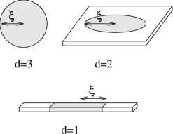
FIG. 1.: The Kondo sreening cloud in different dimensions.

FIG. 2.: The infinite half space of homogeneously dispersed host atoms with spin-orbit interaction and the magnetic impurity in a distance $d$ measured from the surface.

FIG. 3.: The electron propagator leaving and arriving at the impurity. The heavy lines represent the localized d-electron propagators, and $V$ and $\lambda$ indicate the hybridization with the localized orbital and the spin-orbit interaction, respectively. The indices are according to the local system.

FIG. 4.: The self-energy diagrams for the impurity spin. The double line represents the spin, the single one the conduction electrons. The solid circles stand for the exchange interaction and the $\times$ labelled by $n$ for the effective spin-orbit interaction on the orbital of the host atom at ${\bf R}_{n}$.

FIG. 5.: Carrying out the average over the homogeneously dispersed host atoms, the different shells with constant radiusis $R_{n}$ and $R_{n^{\prime}}$ are shown which can be restricted by the surface.

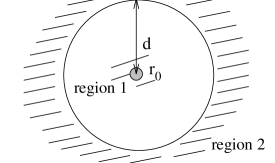
FIG. 6.: The two dominating regions contributing to the double integral. Region 2 is formed by those shells of smallest radia which are not complete due to the presence of the surface. Region 1 is around the impurity of smallest radia with short range rutoff $r_{0}$.

FIG. 7.: The levels for $S=2$ as the function of the external magnetic field (a) without and (b) with surface anisotropy.

TABLE I.: The analytical part of diagram Fig. 5 b) in function of $x={\omega\over D}$.